Data Structures & Algorithms in Java PHẦN 10 ppsx

- 478 -


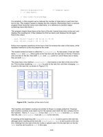
Figure 14.2: The GraphW Workshop applet






Now find this graph's minimum spanning tree by stepping through the algorithm with the
Tree key. The result should be the minimum spanning tree shown in Figure 14.3.









Figure 14.3: The minimum spanning tree






The applet should discover that the minimum spanning tree consists of the edges AD,
AB, BE, EC, and CF, for a total edge weight of 28. The order in which the edges are

specified is unimportant. If you start at a different vertex you will create a tree with the
same edges, but in a different order.





Send Out the Surveyors




The algorithm for constructing the minimum spanning tree is a little involved, so we're
going to introduce it using an analogy involving cable TV employees. You are one
employee—a manager, of course—and there are also various surveyors.





A computer algorithm (unless perhaps it's a neural network) doesn't "know" about all the
data in a given problem at once; it can't deal with the big picture. It must acquire the data
little by little, modifying its view of things as it goes along. With graphs, algorithms tend to
start at some vertex and work outward, acquiring data about nearby vertices before
finding out about vertices farther away. We've seen examples of this in the depth-first and
breadth-first searches in the last chapter.

In a similar way, we're going to assume that you don't start out knowing the costs of
installing the cable TV line between all the pairs of towns in Magnaguena. Acquiring this
information takes time. That's where the surveyors come in.





Starting in Ajo




You start by setting up an office in Ajo. (You could start in any town, but Ajo has the best
restaurants.) Only two towns are reachable from Ajo: Bordo and Danza (refer to Figure
14.1). You hire two tough, jungle-savvy surveyors and send them out along the
dangerous wilderness trails, one to Bordo and one to Danza. Their job is to determine the
cost of installing cable along these routes.





The first surveyor arrives in Bordo, having completed her survey, and calls you on her
cellular phone; she says it will cost 6 million dollars to install the cable link between Ajo
and Bordo. The second surveyor, who has had some trouble with crocodiles, reports a
little later from Danza that the Ajo–Danza link, which crosses more level country, will cost
only 4 million dollars. You make a list:

•

Ajo–Danza, $4 million




•

Ajo–Bordo, $6 million




You always list the links in order of increasing cost; we'll see why this is a good idea


- 479 -
soon.



Building the Ajo–Danza Link

At this point you figure you can send out the construction crew to actually install the cable
from Ajo to Danza. How can you be sure the Ajo–Danza route will eventually be part of
the cheapest solution (the minimum spanning tree)? So far, you only know the cost of two
links in the system. Don't you need more information?





To get a feel for this situation, try to imagine some other route linking Ajo to Danza that
would be cheaper than the direct link. If it doesn't go directly to Danza, this other route
must go through Bordo and circle back to Danza, possibly via one or more other towns.
But you already know the link to Bordo is more expensive, at 6 million dollars,than the
link to Danza, at 4. So even if the remaining links in this hypothetical circle route are
cheap, as shown in Figure 14.4, it will still be more expensive to get to Danza by going
through Bordo. Also, it will be more expensive to get to towns on the circle route, like X,
by going through Bordo than by going through Danza.










Figure 14.4: Hypothetical circle route

We conclude that the Ajo–Danza route will be part of the minimum spanning tree. This
isn't a formal proof (which is beyond the scope of this book), but it does suggest your
best bet is to pick the cheapest link. So you build the Ajo–Danza link and install an office
in Danza.





Why do you need an office? Due to a Magnaguena government regulation, you must
install an office in a town before you can send out surveyors from that town to adjacent
towns. In graph terms, you must add a vertex to the tree before you can learn the weight
of the edges leading away from that vertex. All towns with offices are connected by cable
with each other; towns with no offices are not yet connected.





Building the Ajo–Bordo Link




Once you've completed the Ajo–Danza link and built your office in Danza, you can send

out surveyors from Danza to all the towns reachable from there. These are Bordo, Colina,
and Erizo. The surveyors reach their destinations and report back costs of 7, 8, and 12
million dollars, respectively. (Of course you don't send a surveyor to Ajo because you've
already surveyed the Ajo–Danza route and installed its cable.)





Now you know the costs of four links from towns with offices to towns with no offices:




•

Ajo–Bordo, $6 million




•

Danza–Bordo, $7 million




•

Danza–Colina, $8 million




•

Danza–Erizo, $12 million




- 480 -

Why isn't the Ajo–Danza link still on the list? Because you've already installed the cable
there; there's no point giving any further consideration to this link. The route on which a
cable has just been installed is always removed from the list.





At this point it may not be obvious what to do next. There are many potential links to
choose from. What do you imagine is the best strategy now? Here's the rule:




REMEMBER

Rule: From the list, always pick the cheapest edge.




Actually, you already followed this rule when you chose which route to follow from Ajo;
the Ajo–Danza edge was the cheapest. Here the cheapest edge is Ajo–Bordo, so you
install a cable link from Ajo to Bordo for a cost of 6 million dollars, and build an office in
Bordo.





Let's pause for a moment and make a general observation. At a given time in the cable
system construction, there are three kinds of towns:





1.

Towns that have offices and are linked by cable. (In graph terms they're in the
minimum spanning tree.)

2.

Towns that aren't linked yet and have no office, but for which you know the cost to
link them to at least one town with an office. We can call these "fringe" towns.




3.

Towns you don't know anything about.




At this stage, Ajo, Danza, and Bordo are in category 1, Colina and Erizo are in category
2, and Flor is in category 3, as shown in Figure 14.5. As we work our way through the
algorithm, towns move from category 3 to 2, and from 2 to 1.










Figure 14.5: Partway through the minimum spanning tree algorithm

Building the Bordo–Erizo Link




At this point, Ajo, Danza, and Bordo are connected to the cable system and have offices.
You already know the costs from Ajo and Danza to towns in category 2, but you don't
know these costs from Bordo. So from Bordo you send out surveyors to Colina and Erizo.
They report back costs of 10 to Colina and 7 to Erizo. Here's the new list:





•

Bordo–Erizo, $7 million




•

Danza–Colina, $8 million

•

Bordo–Colina, $10 million




•

Danza–Erizo, $12 million



- 481 -


The Danza–Bordo link was on the previous list but is not on this one because, as we
noted, there's no point in considering links to towns that are already connected, even by
an indirect route.





From this list we can see that the cheapest route is Bordo–Erizo, at 7 million dollars. You
send out the crew to install this cable link, and you build an office in Erizo (refer to Figure

14.3).




Building the Erizo–Colina Link




From Erizo the surveyors report back costs of 5 to Colina and 7 to Flor. The Danza–Erizo
link from the previous list must be removed because Erizo is now a connected town. Your
new list is





•

Erizo–Colina, $5 million




•

Erizo–Flor, $7 million

•

Danza–Colina, $8 million




•

Bordo–Colina, $10 million




The cheapest of these links is Erizo–Colina, so you built this link and install an office in
Colina.





And, Finally, the Colina–Flor Link




The choices are narrowing. After removing already linked towns, your list now shows only

•

Colina–Flor, $6 million




•

Erizo–Flor, $7 million




You install the last link of cable from Colina to Flor, build an office in Flor, and you're
done. You know you're done because there's now an office in every town. You've
constructed the cable route Ajo–Danza, Ajo–Bordo, Bordo–Erizo, Erizo–Colina, and
Colina–Flor, as shown earlier in Figure 14.3
. This is the cheapest possible route linking
the six towns of Magnaguena.





Creating the Algorithm

Using the somewhat fanciful idea of installing a cable TV system, we've shown the main
ideas behind the minimum spanning tree for weighted graphs. Now let's see how we'd go
about creating the algorithm for this process.





The Priority Queue




The key activity in carrying out the algorithm, as described in the cable TV example, was
maintaining a list of the costs of links between pairs of cities. We decided where to build
the next link by selecting the minimum of these costs.





A list in which we repeatedly select the minimum value suggests a priority queue as an
appropriate data structure, and in fact this turns out to be an efficient way to handle the
minimum spanning tree problem. Instead of a list or array, we use a priority queue. In a
serious program this priority queue might be based on a heap, as described in Chapter
12, "Heaps." This would speed up operations on large priority queues. However, in our

- 482 -
demonstration program we'll use a priority queue based on a simple array.



Outline of the Algorithm




Let's restate the algorithm in graph terms (as opposed to cable TV terms):




Start with a vertex, put it in the tree. Then repeatedly do the following:




1.

Find all the edges from the newest vertex to other vertices that aren't in the tree. Put
these edges in the priority queue.

2.

Pick the edge with the lowest weight, and add this edge and its destination vertex to
the tree.





Do these steps until all the vertices are in the tree. At that point, you're done.




In step 1, "newest" means most recently installed in the tree. The edges for this step can
be found in the adjacency matrix. After step 1, the list will contain all the edges from
vertices in the tree to vertices on the fringe.





Extraneous Edges




In maintaining the list of links, we went to some trouble to remove links that led to a town
that had recently become connected. If we didn't do this, we would have ended up
installing unnecessary cable links.

In a programming algorithm we must likewise make sure that we don't have any edges in
the priority queue that lead to vertices that are already in the tree. We could go through
the queue looking for and removing any such edges each time we added a new vertex to
the tree. As it turns out, it is easier to keep only one edge from the tree to a given fringe
vertex in the priority queue at any given time. That is, the queue should contain only one
edge to each category 2 vertex.





You'll see that this is what happens in the GraphW Workshop applet. There are fewer
edges in the priority queue than you might expect; just one entry for each category 2
vertex. Step through the minimum spanning tree for Figure 14.1
and verify that this is
what happens. Table 14.1 shows how edges with duplicate destinations have been
removed from the priority queue.





Table 14.1: Edge pruning

Step Number



Unpruned Edge
List



Pruned Edge List
(in PriorityQueue)



Duplicate
Removed from
Priority Queue

1



AB6, AD4



AB6, AD4








2



DE12, DC8, DB7,
AB6

DE12, DC8, AB6



DB7(AB6)





3



DE12, BC10, DC8,
BE7



DC8, BE7



DE12(BE7),
BC10(DC8)

- 483 -

4


BC10, DC8, EF7,
EC5


EF7, EC5


BC10(EC5),
DC8(EC5)




5



EF7, CF6

CF6



EF7











Remember that an edge consists of a letter for the source (starting) vertex of the edge, a
letter for the destination (ending vertex), and a number for the weight. The second
column in this table corresponds to the lists you kept when constructing the cable TV
system. It shows all edges from category 1 vertices (those in the tree) to category 2
vertices (those with at least one known edge from a category 1 vertex).





The third column is what you see in the priority queue when you run the GraphW applet.
Any edge with the same destination vertex as another edge, and which has a greater
weight, has been removed.

The fourth column shows the edges that have been removed, and, in parentheses, the
edge with the smaller weight that superseded it and remains in the queue. Remember
that as you go from step to step the last entry on the list is always removed because this
edge is added to the tree.





Looking for Duplicates in the Priority Queue




How do we make sure there is only one edge per category 2 vertex? Each time we add
an edge to the queue, we make sure there's no other edge going to the same destination.
If there is, we keep only the one with the smallest weight.





This necessitates looking through the priority queue item by item, to see if there's such a
duplicate edge. Priority queues are not designed for random access, so this is not an
efficient activity. However, violating the spirit of the priority queue is necessary in this

situation.





Java Code




The method that creates the minimum spanning tree for a weighted graph, mstw(),
follows the algorithm outlined above. As in our other graph programs, it assumes there's
a list of vertices in vertexList[], and that it will start with the vertex at index 0. The
currentVert variable represents the vertex most recently added to the tree. Here's the
code for mstw():





public void mstw() // minimum spanning tree



{



currentVert = 0; // start at 0

while(nTree < nVerts-1) // while not all verts in tree



{ // put currentVert in tree



vertexList[currentVert].isInTree = true;



nTree++;





// insert edges adjacent to currentVert into PQ



for(int j=0; j<nVerts; j++) // for each vertex,

{



if(j==currentVert) // skip if it's us



continue;



if(vertexList[j].isInTree) // skip if in the tree



- 484 -

continue;



int distance = adjMat[currentVert][j];



if( distance == INFINITY) // skip if no edge

continue;



putInPQ(j, distance); // put it in PQ (maybe)



}



if(thePQ.size()==0) // no vertices in PQ?



{



System.out.println(" GRAPH NOT CONNECTED");



return;



}

// remove edge with minimum distance, from PQ



Edge theEdge = thePQ.removeMin();



int sourceVert = theEdge.srcVert;



currentVert = theEdge.destVert;





// display edge from source to current



System.out.print( vertexList[sourceVert].label );



System.out.print( vertexList[currentVert].label );

System.out.print(" ");



} // end while(not all verts in tree)





// mst is complete



for(int j=0; j<nVerts; j++) // unmark vertices



vertexList[j].isInTree = false;




} // end mstw()

The algorithm is carried out in the while loop, which terminates when all vertices are in
the tree. Within this loop the following activities take place:





1.

The current vertex is placed in the tree.




2.

The edges adjacent to this vertex are placed in the priority queue (if appropriate).




3.

The edge with the minimum weight is removed from priority queue. The destination
vertex of this edge becomes the current vertex.

Let's look at these steps in more detail. In step 1, the currentVert is placed in the tree
by marking its isInTree field.





In step 2, the edges adjacent to this vertex are considered for insertion in the priority
queue. The edges are examined by scanning across the row whose number is
currentVert in the adjacency matrix. An edge is placed in the queue unless one of
these conditions is true:





•

The source and destination vertices are the same.




•

The destination vertex is in the tree.

•

There is no edge to this destination.




If none of these conditions is true, the putInPQ() method is called to put the edge in the
priority queue. Actually, this routine doesn't always put the edge in the queue either, as


- 485 -
we'll see in a moment.



In step 3, the edge with the minimum weight is removed from the priority queue. This
edge and its destination vertex are added to the tree, and the source vertex
(currentVert) and destination vertex are displayed.





At the end of mstw(), the vertices are removed from the tree by resetting their
isInTree variables. That isn't strictly necessary in this program, because only one tree
is created from the data. However, it's good housekeeping to restore the data to its
original form when you finish with it.

As we noted, the priority queue should contain only one edge with a given destination
vertex. The putInPQ() method makes sure this is true. It calls the find() method of
the PriorityQ class, which has been doctored to find the edge with a specified
destination vertex. If there is no such vertex, and find() therefore returns –1, then
putInPQ() simply inserts the edge into the priority queue. However, if such an edge
does exist, putInPQ() checks to see whether the existing edge or the new proposed
edge has the lower weight. If it's the old edge, no change is necessary. If the new one
has a lower weight, the old edge is removed from the queue and the new one is installed.
Here's the code for putInPQ():





public void putInPQ(int newVert, int newDist)



{



// is there another edge with the same destination vertex?



int queueIndex = thePQ.find(newVert); // got edge's index

if(queueIndex != -1) // if there is one,



{ // get edge



Edge tempEdge = thePQ.peekN(queueIndex);



int oldDist = tempEdge.distance;



if(oldDist > newDist) // if new edge shorter,



{



thePQ.removeN(queueIndex); // remove old edge

Edge theEdge = new Edge(currentVert, newVert,
newDist);




thePQ.insert(theEdge); // insert new edge



}



// else no action; just leave the old vertex there



} // end if



else // no edge with same destination vertex



{ // so insert new one

Edge theEdge = new Edge(currentVert, newVert, newDist);



thePQ.insert(theEdge);



}




} // end putInPQ()




The mstw.java Program




The PriorityQ class uses an array to hold the members. As we noted, in a program
dealing with large graphs a heap would be more appropriate than the array shown here.
The PriorityQ class has been augmented with various methods. It can, as we've seen,
find an edge with a given destination vertex with find(). It can also peek at an arbitrary
member with peekN() and remove an arbitrary member with removeN(). Most of the
rest of this program you've seen before. Listing 14.1 shows the complete mstw.java

program.





- 486 -

Listing 14.1 The mstw.java Program




// mstw.java



// demonstrates minimum spanning tree with weighted graphs



// to run this program: C>java MSTWApp



import java.awt.*;



////////////////////////////////////////////////////////////////

class Edge



{



public int srcVert; // index of a vertex starting edge



public int destVert; // index of a vertex ending edge



public int distance; // distance from src to dest





public Edge(int sv, int dv, int d) // constructor



{

srcVert = sv;



destVert = dv;



distance = d;



}



} // end class Edge




////////////////////////////////////////////////////////////////




class PriorityQ

{



// array in sorted order, from max at 0 to min at size-1



private final int SIZE = 20;



private Edge[] queArray;



private int size;





public PriorityQ() // constructor



{

queArray = new Edge[SIZE];



size = 0;



}





public void insert(Edge item) // insert item in sorted
order




{



int j;

for(j=0; j<size; j++) // find place to insert



if( item.distance >= queArray[j].distance )



break;





for(int k=size-1; k>=j; k ) // move items up



queArray[k+1] = queArray[k];





queArray[j] = item; // insert item

size++;



}





public Edge removeMin() // remove minimum item



- 487 -

{ return queArray[ size]; }





public void removeN(int n) // remove item at n



{

for(int j=n; j<size-1; j++) // move items down



queArray[j] = queArray[j+1];



size ;



}





public Edge peekMin() // peek at minimum item



{ return queArray[size-1]; }





public int size() // return number of items

{ return size; }





public boolean isEmpty() // true if queue is empty



{ return (size==0); }





public Edge peekN(int n) // peek at item n



{ return queArray[n]; }





public int find(int findDex) // find item with specified

{ // destVert value



for(int j=0; j<size; j++)



if(queArray[j].destVert == findDex)



return j;



return -1;



}



} // end class PriorityQ

////////////////////////////////////////////////////////////////




class Vertex



{



public char label; // label (e.g. 'A')



public boolean isInTree;




//
-

public Vertex(char lab) // constructor



{



label = lab;



isInTree = false;



}




//
-




} // end class Vertex

////////////////////////////////////////////////////////////////




class Graph



{



- 488 -

private final int MAX_VERTS = 20;



private final int INFINITY = 1000000;



private Vertex vertexList[]; // list of vertices



private int adjMat[][]; // adjacency matrix

private int nVerts; // current number of vertices



private int currentVert;



private PriorityQ thePQ;



private int nTree; // number of verts in tree




//
-




public Graph() // constructor

{



vertexList = new Vertex[MAX_VERTS];



// adjacency matrix



adjMat = new int[MAX_VERTS][MAX_VERTS];



nVerts = 0;



for(int j=0; j<MAX_VERTS; j++) // set adjacency



for(int k=0; k<MAX_VERTS; k++) // matrix to 0



adjMat[j][k] = INFINITY;

thePQ = new PriorityQ();



} // end constructor




//
-




public void addVertex(char lab)



{



vertexList[nVerts++] = new Vertex(lab);



}

//
-




public void addEdge(int start, int end, int weight)



{



adjMat[start][end] = weight;



adjMat[end][start] = weight;



}

//
-




public void displayVertex(int v)



{



System.out.print(vertexList[v].label);



}




//
-

public void mstw() // minimum spanning tree



{



currentVert = 0; // start at 0





while(nTree < nVerts-1) // while not all verts in tree



{ // put currentVert in tree



vertexList[currentVert].isInTree = true;



- 489 -

nTree++;

// insert edges adjacent to currentVert into PQ



for(int j=0; j<nVerts; j++) // for each vertex,



{



if(j==currentVert) // skip if it's us



continue;



if(vertexList[j].isInTree) // skip if in the tree



continue;

int distance = adjMat[currentVert][j];



if( distance == INFINITY) // skip if no edge



continue;



putInPQ(j, distance); // put it in PQ (maybe)



}



if(thePQ.size()==0) // no vertices in PQ?



{

System.out.println(" GRAPH NOT CONNECTED");



return;



}



// remove edge with minimum distance, from PQ



Edge theEdge = thePQ.removeMin();



int sourceVert = theEdge.srcVert;



currentVert = theEdge.destVert;

// display edge from source to current



System.out.print( vertexList[sourceVert].label );



System.out.print( vertexList[currentVert].label );



System.out.print(" ");



} // end while(not all verts in tree)





// mst is complete



for(int j=0; j<nVerts; j++) // unmark vertices

vertexList[j].isInTree = false;



} // end mstw




//
-




public void putInPQ(int newVert, int newDist)



{



// is there another edge with the same destination
vertex?




int queueIndex = thePQ.find(newVert);

if(queueIndex != -1) // got edge's index



{



Edge tempEdge = thePQ.peekN(queueIndex); // get edge



int oldDist = tempEdge.distance;



if(oldDist > newDist) // if new edge shorter,



{



thePQ.removeN(queueIndex); // remove old edge

Edge theEdge =



new Edge(currentVert, newVert,
newDist);




thePQ.insert(theEdge); // insert new edge



- 490 -

}



// else no action; just leave the old vertex there



} // end if



else // no edge with same destination vertex

{ // so insert new one



Edge theEdge = new Edge(currentVert, newVert,
newDist);




thePQ.insert(theEdge);



}



} // end putInPQ()




//
-

} // end class Graph




////////////////////////////////////////////////////////////////




class MSTWApp



{



public static void main(String[] args)



{



Graph theGraph = new Graph();

theGraph.addVertex('A'); // 0 (start for mst)



theGraph.addVertex('B'); // 1



theGraph.addVertex('C'); // 2



theGraph.addVertex('D'); // 3



theGraph.addVertex('E'); // 4



theGraph.addVertex('F'); // 5





theGraph.addEdge(0, 1, 6); // AB 6

theGraph.addEdge(0, 3, 4); // AD 4



theGraph.addEdge(1, 2, 10); // BC 10



theGraph.addEdge(1, 3, 7); // BD 7



theGraph.addEdge(1, 4, 7); // BE 7



theGraph.addEdge(2, 3, 8); // CD 8



theGraph.addEdge(2, 4, 5); // CE 5



theGraph.addEdge(2, 5, 6); // CF 6

theGraph.addEdge(3, 4, 12); // DE 12



theGraph.addEdge(4, 5, 7); // EF 7





System.out.print("Minimum spanning tree: ");



theGraph.mstw(); // minimum spanning tree



System.out.println();



} // end main()



} // end class MSTWApp

///////////////////////////////////////////////////////////////




The main() routine in class MSTWApp creates the tree in Figure 14.1. Here's the output:




Minimum spanning tree: AD AB BE EC CF


The Shortest-Path Problem



- 491 -


Perhaps the most commonly encountered problem associated with weighted graphs is
that of finding the shortest path between two given vertices. The solution to this problem
is applicable to a wide variety of real-world situations, from the layout of printed circuit
boards to project scheduling. It is a more complex problem than we've seen before, so
let's start by looking at a (somewhat) real-world scenario in the same mythical country of
Magnaguena introduced in the last section.

The Railroad Line




This time we're concerned with railroads rather than cable TV. However, this project is
not as ambitious as the last one. We're not going to build the railroad; it already exists.
We just want to find the cheapest route from one city to another.





The railroad charges passengers a fixed fare to travel between any two towns. These
fares are shown in Figure 14.6. That is, from Ajo to Bordo is $50, from Bordo to Danza is
$90, and so on. These rates are the same whether the ride between two towns is part of
a longer itinerary or not (unlike the situation with today's airline fares).





The edges in Figure 14.6 are directed. They represent single-track railroad lines, on
which (in the interest of safety) travel is permitted in only one direction. For example, you
can go directly from Ajo to Bordo, but not from Bordo to Ajo.

Figure 14.6: Train fares in Magnaguena






Although in this situation we're interested in the cheapest fares, the graph problem is
nevertheless always referred to as the shortest path problem. Here shortest doesn't
necessarily mean shortest in terms of distance; it can also mean cheapest, fastest, or
best route by some other measure.





Cheapest Fares




There are several possible routes between any two towns. For example, to take the train
from Ajo to Erizo you could go through Danza, or you could go through Bordo and Colina,

or through Danza and Colina, or you could take several other routes. (It's not possible to
reach the town of Flor by rail because it lies beyond the rugged Sierra Descaro range, so
it doesn't appear on the graph. This is fortunate, because it reduces the size of certain
lists we'll need to make.)





The shortest-path problem is, for a given starting point and destination, what's the
cheapest route? In Figure 14.6, you can see (with a little mental effort) that the cheapest
route from Ajo to Erizo passes through Danza and Colina; it will cost you $140.





A Directed, Weighted Graph




As we noted, our railroad has only single-track lines, so you can go in only one direction
between any two cities. This corresponds to a directed graph. We could have portrayed
the more realistic situation in which you can go either way between two cities for the
same price; this would correspond to a nondirected graph. However, the


- 492 -
shortest-path problem is similar in these cases, so for variety we'll show how it looks in a

directed graph.



Dijkstra's Algorithm




The solution we'll show for the shortest-path problem is called Dijkstra's Algorithm, after
Edsger Dijkstra, who first described it in 1959. This algorithm is based on the adjacency
matrix representation of a graph. Somewhat surprisingly, it finds not only the shortest
path from one specified vertex to another, but the shortest paths from the specified vertex
to all the other vertices.





Agents and Train Rides




To see how Dijkstra's Algorithm works, imagine that you want to find the cheapest way to
travel from Ajo to all the other towns in Magnaguena. You (and various agents you will
hire) are going to play the role of the computer program carrying out Dijkstra's Algorithm.
Of course in real life you could probably obtain a schedule from the railroad with all the
fares. The Algorithm, however, must look at one piece of information at a time, so (as in
the last section) we'll assume that you are similarly unable to see the big picture.

At each town, the stationmaster can tell you how much it will cost to travel to the other
towns that you can reach directly (that is, in a single ride, without passing through
another town). Alas, he cannot tell you the fares to towns further than one ride away. You
keep a notebook, with a column for each town. You hope to end up with each column
showing the cheapest route from your starting point to that town.





The First Agent: In Ajo




Eventually you're going to place an agent in every town; this agent's job is to obtain
information about ticket costs to other towns. You yourself are the agent in Ajo.




All the stationmaster in Ajo can tell you is that it will cost $50 to ride to Bordo, and $80 to
ride to Danza. You write this in your notebook, as shown in Table 14.2.

Table 14.2:
Step 1: An agent at Ajo











From Ajo to



Bordo



Colina


Danza

Erizo











Step 1



50 (via Ajo)



inf


80 (via Ajo)



inf

The entry "inf" is short for "infinity," and means that you can't get from Ajo to the town
shown in the column head, or at least that you don't yet know how to get there. (In the
algorithm infinity will be represented by a very large number, which will help with
calculations, as we'll see.) The entries in the table in parentheses are the last town visited
before you arrive at the various destinations. We'll see later why this is good to know.
What do you do now? Here's the rule you'll follow:





REMEMBER



Rule: Always send an agent to the town whose overall fare from the starting point (Ajo) is
the cheapest.



- 493 -

You don't consider towns that already have an agent. Notice that this is not the same rule
as that used in the minimum spanning tree problem (the cable TV installation). There,
you picked the least expensive single link (edge) from the connected towns to an
unconnected town. Here, you pick the least expensive total route from Ajo to a town with
no agent. In this particular point in your investigation these two approaches amount to the
same thing, because all known routes from Ajo consist of only one edge; but as you send
agents to more towns, the routes from Ajo will become the sum of several direct edges.





The Second Agent: In Bordo




The cheapest fare from Ajo is to Bordo, at $50. So you hire a passerby and send him to
Bordo, where he'll be your agent. Once he's there, he calls you by telephone, and tells
you that the Bordo stationmaster says it costs $60 to ride to Colina and $90 to Danza.





Doing some quick arithmetic, you figure it must be $50 plus $60, or $110 to go from Ajo
to Colina via Bordo, so you modify the entry for Colina. You also can see that, going via
Bordo, it must be $50 plus $90, or $140, from Ajo to Danza. However—and this is a key

point—you already know it's only $80 going directly from Ajo to Danza. You only care
about the cheapest route from Ajo, so you ignore the more expensive route, leaving this
entry as it was. The resulting notebook entries are shown in the last row in Table 14.3.
Figure 14.7 shows the situation geographically.





Table 14.3:
Step 2: Agents at Ajo and Bordo










From Ajo to



Bordo

Colina



Danza



Erizo











Step 1



50 (via Ajo)




inf

80 (via Ajo)



inf





Step 2



50 (via Ajo)*




110 (via Bordo)


80 (via Ajo)



inf

Figure 14.7: Following step 2 in the shortest-path algorithm






Once we've installed an agent in a town, we can be sure that the route taken by the
agent to get to that town is the cheapest route. Why? Consider the present case. If there
were a cheaper route than the direct one from Ajo to Bordo, it would need to go through
some other town. But the only other way out of Ajo is to Danza, and that ride is already
more expensive than the direct route to Bordo. Adding additional fares to get from Danza

- 494 -
to Bordo would make the Danza route still more expensive.



From this we decide that from now on we won't need to update the entry for the cheapest
fare from Ajo to Bordo. This fare will not change, no matter what we find out about other
towns. We'll put an * next to it to show that there's an agent in the town and that the
cheapest fare to it is fixed.





Three Kinds of Town




As in the minimum spanning tree algorithm, we're dividing the towns into three
categories:





1.

Towns in which we've installed an agent; they're in the tree.

2.

Towns with known fares from towns with an agent; they're on the fringe.




3.

Unknown towns.




At this point Ajo and Bordo are category 1 towns because there are agents there.
Category 1 towns form a tree consisting of paths that all begin at the starting vertex and
that each end on a different destination vertex. (This is not the same tree, of course, as a
minimum spanning tree.)





Some other towns have no agents, but you know the fares to them because you have
agents in adjacent category 1 towns. You know the fare from Ajo to Danza is $80, and
from Bordo to Colina is $60. Because the fares to them are known, Danza and Colina are
category 2 (fringe) towns.

You don't know anything yet about Erizo, it's an "unknown" town. Figure 14.7 shows
these categories at the current point in the algorithm.




As in the minimum spanning tree algorithm, the algorithm moves towns from the
unknown category to the fringe category, and from the fringe category to the tree, as it
goes along.





The Third Agent: In Danza




At this point, the cheapest route you know that goes from Ajo to any town without an
agent is $80, the direct route from Ajo to Danza. Both the Ajo–Bordo–Colina route at
$110, and the Ajo–Bordo–Danza route at $140, are more expensive.

You hire another passerby and send her to Danza with an $80 ticket. She reports that
from Danza it's $20 to Colina and $70 to Erizo. Now you can modify your entry for Colina.
Before, it was $110 from Ajo, going via Bordo. Now you see you can reach Colina for
only $100, going via Danza. Also, you now know a fare from Ajo to the previously
unknown Erizo: it's $150, via Danza. You note these changes, as shown in Table 14.4
and Figure 14.8.





Table 14.4:
Step 3: Agents at Ajo, Bordo, and Danza










From Ajo
to

Bordo




Colina


Danza


Erizo














- 495 -

Step 1

50 (via Ajo)


inf

80 (via Ajo)

inf




Step 2



50 (via Ajo)*




110 (via Bordo)


80 (via Ajo)


inf

Step 3



50 (via Ajo)*




100 (via Danza)


80 (via Ajo)*


150 (via Danza)

Figure 14.8: Following step 3 in the shortest-path algorithm






The Fourth Agent: In Colina




Now the cheapest path to any town without an agent is the $100 trip from Ajo to Colina,
going via Danza. Accordingly, you dispatch an agent over this route to Colina. He reports
that it's $40 from there to Erizo. Now you can calculate that, because Colina is $100 from
Ajo (via Danza), and Erizo is $40 from Colina, you can reduce the minimum Ajo-to-Erizo
fare from $150 (the Ajo–Danza–Erizo route) to $140 (the Ajo–Danza–Colina–Erizo route).
You update your notebook accordingly, as shown in Table 14.5
and Figure 14.9.

Table 14.5:
Step 4: Agents in Ajo, Bordo, Danza, and Colina










From Ajo to



Bordo




Colina



Danza



Erizo

Step 1



50 (via Ajo)




inf



80 (via Ajo)



inf

Step 2



50 (via Ajo)*




110 (via Bordo)



80 (via Ajo)



inf





Step 3

50 (via Ajo)*




100 (via
Danza)



80 (via Ajo)*



150 (via Danza)





Step 4



50 (via Ajo)*

100 (via
Danza)*




80 (via Ajo)*



140 (via Colina)











- 496 -






Figure 14.9: Following step 4 in the shortest-path algorithm

The Last Agent: In Erizo




The cheapest path from Ajo to any town you know about that doesn't have an agent is
now $140 to Erizo, via Danza and Colina. You dispatch an agent to Erizo, but she reports
that there are no routes from Erizo to towns without agents. (There's a route to Bordo, but
Bordo has an agent.) Table 14.6 shows the final line in your notebook; all you've done is
add a star to the Erizo entry to show there's an agent there.





Table 14.6:
Step 5: Agents in Ajo, Bordo, Danza, Colina, and Erizo

From Ajo to



Bordo




Colina



Danza



Erizo

Step 1



50 (via Ajo)




inf



80 (via Ajo)



inf





Step 2



50 (via Ajo)*

110 (via Bordo)



80 (via Ajo)



inf





Step 3



50 (via Ajo)*




100 (via
Danza)

80 (via Ajo)*



150 (via Danza)





Step 4



50 (via Ajo)*




100 (via
Danza)*




80 (via Ajo)*

140 (via Colina)





Step 5



50 (via Ajo)*




100 (via
Danza)*



80 (via Ajo)*



140 (via Colina)*

When there's an agent in every town, you know the fares from Ajo to every other town.
So you're done. With no further calculations, the last line in your notebook shows the
cheapest routes from Ajo to all other towns.





This narrative has demonstrated the essentials of Dijkstra's Algorithm. The key points are




•

Each time you send an agent to a new town, you use the new information provided by
that agent to revise your list of fares. Only the cheapest fare (that you know about)
from the starting point to a given town is retained.

•

You always send the new agent to the town that has the cheapest path from the
starting point. (Not the cheapest edge from any town with an agent, as in the minimum


- 497 -
spanning tree.)



Using the Workshop Applet




Let's see how this looks using the GraphDW (for Directed and Weighted) Workshop
applet. Use the applet to create the graph from Figure 14.6. The result should look
something like Figure 14.10. (We'll see how to make the table appear below the graph in
a moment.) This is a weighted, directed graph, so to make an edge, you must type a
number before dragging, and you must drag in the correct direction, from the start to the
destination.

Figure 14.10: The railroad scenario in GraphDW






When the graph is complete, click the Path button, and when prompted, click the A
vertex. A few more clicks on Path will place A in the tree, shown with a red circle around
A.





The Shortest-Path Array




An additional click will install a table under the graph, as you can see in Figure 14.10.
The corresponding message near the top of the figure is Copied row A from
adjacency matrix to shortest-path array. Dijkstra's Algorithm starts by
copying the appropriate row of the adjacency matrix (that is, the row for the starting
vertex) to an array. (Remember that you can examine the adjacency matrix at any time
by pressing the View button.)

This array is called the "shortest-path" array. It corresponds to the most recent row of
notebook entries you made while determining the cheapest train fares in Magnaguena.
This array will hold the current versions of the shortest paths to the other vertices, which
we can call the destination vertices. These destination vertices are represented by the
column heads in the table.





Table 14.7:
Step 1: The Shortest-Path Array










A

B




C


D


E











inf(A)



50(A)

inf(A)


80(A)


inf(A)





- 498 -







In the applet, the shortest-path figures in the array are followed by the parent vertex
enclosed in parentheses. The parent is the vertex you reached just before you reached
the destination vertex. In this case the parents are all A because we've only moved one
edge away from A.

If a fare is unknown (or meaningless, as from A to A) it's shown as infinity, represented by
"inf," as in the rail-fare notebook entries. Notice that the column heads of those vertices
that have already been added to the tree are shown in red. The entries for these columns
won't change.





Minimum Distance




Initially, the algorithm knows the distances from A to other vertices that are exactly one
edge from A. Only B and D are adjacent to A, so they're the only ones whose distances
are shown. The algorithm picks the minimum distance. Another click on Path will show
you the message





Minimum distance from A is 50, to vertex B




The algorithm adds this vertex to the tree, so the next click will show you

Added vertex B to tree




Now B is circled in the graph, and the B column head is in red. The edge from A to B is
made darker to show it's also part of the tree.





Column by Column in the Shortest-Path Array




Now the algorithm knows, not only all the edges from A, but the edges from B as well. So
it goes through the shortest-path array, column by column, checking whether a shorter
path than that shown can be calculated using this new information. Vertices that are
already in the tree, here A and B, are skipped. First column C is examined.

You'll see the message




To C: A to B (50) plus edge BC (60) less than A to C (inf)




The algorithm has found a shorter path to C than that shown in the array. The array
shows infinity in the C column. But from A to B is 50 (which the algorithm finds in the B
column in the shortest-path array) and from B to C is 60 (which it finds in row B column C
in the adjacency matrix). The sum is 110. The 110 distance is less than infinity, so the
algorithm updates the shortest-path array for column C, inserting 110.





This is followed by a B in parentheses, because that's the last vertex before reaching C;
B is the parent of C.





Next the D column is examined. You'll see the message

To D: A to B (50) plus edge BD (90) greater than or equal to A
to D (80)





The algorithm is comparing the previously shown distance from A to D, which is 80 (the
direct route), with a possible route via B (that is, A–B–D). But path A–B is 50 and edge
BD is 90, so the sum is 140. This is bigger than 80, so 80 is not changed.





- 499 -

For column E, the message is




To E: A to B (50) plus edge BE (inf) greater than or equal to A
to E

(inf)




The newly calculated route from A to E via B (50 plus infinity) is still greater than or equal
to the current one in the array (infinity), so the E column is not changed. The shortest-
path array now looks like Table 14.8.





Table 14.8:
Step 2: The Shortest-Path Array










A

B




C



D



E











inf(A)



50(A)

110(B)



80(A)



inf(A)











Now we can see more clearly the role played by the parent vertex shown in parentheses
after each distance. Each column shows the distance from A to an ending vertex. The
parent is the immediate predecessor of the ending vertex along the path from A. In
column C, the parent vertex is B, meaning that the shortest path from A to C passes
through B just before it gets to C. This information is used by the algorithm to place the
appropriate edge in the tree. (When the distance is infinity, the parent vertex is

meaningless and is shown as A.)





New Minimum Distance




Now that the shortest-path array has been updated, the algorithm finds the shortest
distance in the array, as you will see with another Path key press. The message is




Minimum distance from A is 80, to vertex D




Accordingly, the message




Added vertex D to tree

appears and the new vertex and edge AC are added to the tree.




Do It Again, and Again




Now the algorithm goes through the shortest-path array again, checking and updating the
distances for destination vertices not in the tree; only C and E are still in this category.
Column C and E are both updated. The result is shown in Table 14.9.





Table 14.9:
Step 3: The Shortest-Path Array

- 500 -

A


B


C

D


E

inf(A)



50(A)




100(D)


80(A)



150(D)











The shortest path from A to a non-tree vertex is 100, to vertex C, so C is added to the
tree.

Next time through the shortest-path array, only the distance to E is considered. It can be
shortened by going via C, so we have the entries shown in Table 14.10.





Table 14.10:
Step 4: The Shortest-Path Array










A



B

C


D



E











inf(A)



50(A)

100(D)


80(A)



140(C)











Now the last vertex, E, is added to the tree, and you're done. The shortest-path array
shows the shortest distances from A to all the other vertices. The tree consists of all the
vertices and the edges AB, AD, DC, and CE, shown with thick lines.





You can work backward to reconstruct the sequence of vertices along the shortest path
to any vertex. For the shortest path to E, for example, the parent of E, shown in the array

in parentheses, is C. The predecessor of C, again from the array, is D, and the
predecessor of D is A. So the shortest path from A to E follows the route A–D–C–E.





Experiment with other graphs using GraphDW, starting with small ones. You'll find that
after a while you can predict what the algorithm is going to do, and you'll be on your way
to understanding Dijkstra's Algorithm.





Java Code




The code for the shortest-path algorithm is among the most complex in this book, but
even so it's not beyond mere mortals. We'll look first at a helper class and then at the
chief method that executes the algorithm, path(), and finally at two methods called by
path() to carry out specialized tasks.





The sPath Array and the DistPar Class

As we've seen, the key data structure in the shortest-path algorithm is an array that
keeps track of the minimum distances from the starting vertex to the other vertices
(destination vertices). During the execution of the algorithm these distances are changed,
until at the end they hold the actual shortest distances from the start. In the example
code, this array is called sPath[] (for shortest paths).





As we've seen, it's important to record not only the minimum distance from the starting


- 501 -
vertex to each destination vertex, but also the path taken. Fortunately, the entire path
need not be explicitly stored. It's only necessary to store the parent of the destination
vertex. The parent is the vertex reached just before the destination. We've seen this in
the workshop applet, where, if 100(D) appears in the C column, it means that the
cheapest path from A to C is 100, and D is the last vertex before C on this path.




There are several ways to keep track of the parent vertex, but we choose to combine the
parent with the distance and put the resulting object into the sPath[] array. We call this
class of objects DistPar (for distance-parent).

class DistPar // distance and parent



{ // items stored in sPath array



public int distance; // distance from start to this vertex



public int parentVert; // current parent of this vertex





public DistPar(int pv, int d) // constructor



{

distance = d;



parentVert = pv;



}




}




The path() Method




The path() method carries out the actual shortest-path algorithm. It uses the DistPar
class and the Vertex class, which we saw in the mstw.java program earlier in this
chapter. The path() method is a member of the graph class, which we also saw in
mstw.java in a somewhat different version.

public void path() // find all shortest paths



{



int startTree = 0; // start at vertex 0



vertexList[startTree].isInTree = true;



nTree = 1; // put it in tree





// transfer row of distances from adjMat to sPath



for(int j=0; j<nVerts; j++)

{



int tempDist = adjMat[startTree][j];



sPath[j] = new DistPar(startTree, tempDist);



}





// until all vertices are in the tree



while(nTree < nVerts)



{

int indexMin = getMin(); // get minimum from sPath



int minDist = sPath[indexMin].distance;





if(minDist == INFINITY) // if all infinite



{ // or in tree,



System.out.println("There are unreachable vertices");



break; // sPath is complete



}

- 502 -

else



{ // reset currentVert



currentVert = indexMin; // to closest vert



startToCurrent = sPath[indexMin].distance;



// minimum distance from startTree is



// to currentVert, and is startToCurrent



}

// put current vertex in tree



vertexList[currentVert].isInTree = true;



nTree++;



adjust_sPath(); // update sPath[] array



} // end while(nTree<nVerts)





displayPaths(); // display sPath[] contents

nTree = 0; // clear tree



for(int j=0; j<nVerts; j++)



vertexList[j].isInTree = false;




} // end path()




The starting vertex is always at index 0 of the vertexList[] array. The first task in
path() is to put this vertex into the tree. As the algorithm proceeds we'll be moving othe
r

vertices into the tree as well. The Vertex class contains a flag that indicates whether a
vertex object is in the tree. Putting a vertex in the tree consists of setting this flag and
incrementing nTree, which counts how many vertices are in the tree.

Second, path() copies the distances from the appropriate row of the adjacency matrix
to sPath[]. This is always row 0, because for simplicity we assume 0 is the index of the
starting vertex. Initially, the parent field of all the sPath[] entries is A, the starting
vertex.





We now enter the main while loop of the algorithm. This loop terminates when all the
vertices have been placed in the tree. There are basically three actions in this loop:





1.

Choose the sPath[] entry with the minimum distance.




2.

Put the corresponding vertex (the column head for this entry) in the tree. This
becomes the "current vertex" currentVert.

3.

Update all the sPath[] entries to reflect distances from currentVert.




If path() finds that the minimum distance is infinity, it knows that there are vertices that
are unreachable from the starting point. Why? Because not all the vertices are in the tree
(the while loop hasn't terminated), and yet there's no way to get to these extra vertices;
if there were, there would be a non-infinite distance.





Before returning, path() displays the final contents of sPath[] by calling the
displayPaths() method. This is the only output from the program. Also, path() sets
nTree to 0 and removes the isInTree flags from all the vertices, in case they might be
used again by another algorithm (although they aren't in this program).





Finding the Minimum Distance with getMin()

To find the sPath[] entry with the minimum distance, path() calls the getMin()