DESIGN AND ANALYSIS OF DISTRIBUTED ALGORITHMS phần 7 docx

348 SYNCHRONOUS COMPUTATIONS
Our goal is now to design protocols that can communicate any positive integer
I transmitting k +1 packets and using as little time as possible. Observe that with
k +1 packets the communication sequence is
b
0
: q
1
: b
1
: q
2
: b
2
: : q
k
: b
k
.
We will first of all make a distinction between protocols that do not care about the
content of the transmitted protocols (like C
2
and C
3
) and those (like R
2
and R
3
) that
use those packets to convey information about I .
The first class of protocols are able to tolerate the type of transmission failures

called corruptions. In fact, they use packets only to delimit quanta; as it does not
matter what the content of the packet is (but only that it is being transmitted), these
protocols will work correctly even if the value of the bits in the packets is changed
during transmission. We will call them as corruption-tolerant communicators.
The second class exploits the content of the packets to convey information about
I ; hence, if the value of just one of the bits is changed during transmission, the entire
communication will become corrupted. In other words, these communicators need
reliable transmission for their correctness.
Clearly, the bounds and the optimal solution protocols are different for the two
classes.
We will consider the first class in details; the second types of communicators will
be briefly sketched at the end. As before, we will consider for simplicity the case
when a packet is composed of a single bit, that is c = 1; the results can be easily
generalized to the case c>1.
Corruption-Tolerant Communication If transmissions are subject to corrup-
tions, the value of thereceived packets cannot be reliedupon, and so they are used only
to delimit quanta. Hence, the only meaningful part of the communication sequence
is the k−tuple of quanta
q
1
, q
2
, ,q
k
.
Thus, the (infinite) set Q
k
of all possible k-tuples q
1
, q

2
, ,q
k
, where the q
i
are nonnegative integers, describes all the possible communication sequences.
What we are going to do is to associate to each communication sequence Q[I ] ∈
Q
k
a different integer I. Then, if we want to communicate I , we will use the unique
sequence of quanta described by Q[I ].
To achieve this goal weneed a bijection betweenk-tuples and nonnegative integers.
This is not difficult to do; it is sufficient to establish a total order among tuples as
follows.
Given two k-tuples Q =q
1
,q
2
, ,q
k
 and Q

=q

1
,q

2
, ,q


k
 of positive
integers, we say that Q<Q

if
1.

i
q
i
<

i
q

i
or
2.

i
q
i
=

i
q

i
and q
j

= q

j
for 1 ≤ j<l, and q
l
<q

l
for some index l,1≤
l ≤ k + 1.
COMMUNICATORS, PIPELINE, AND TRANSFORMERS 349
I 0 1 2 3 4 5 6 7 8 9 10
Q[I] 0,0,0 0,0,1 0,1,0 1,0,0 0,0,2 0,1,1 0,2,0 1,0,1 1,1,0 2,0,0 0,0,3
11 12 13 14 15 16 17 18
19 20 21
22
0,1,2 0,2,1 0,3,0 1,0,2 1,1,1
1,2,0 2,0,1 2,1,0 3,0,0 0,0,4 0,1,3 0,2,2
23 24 25 26 27
28 29 30
31 32 33 34
0,3,1 0,4,0
1,0,3 1,1,2 1,2,1 1,3,0 2,0,2 2,1,1 2,2,0 3,0,1 3,1,0 4,0,0
FIGURE 6.9: The first 35 elements of Q
3
according to the total order.
That is, in this total order, all the tuples where the sum of the quanta is t are smaller
than those where the sum is t +1; so, for example 2, 0, 0 is smaller than 1, 1, 1.
If the sum of the quanta is the same, the tuples are lexicographically ordered; so, for
example, 1, 0, 2 is smaller than 1, 1, 1. The ordered list of the first few elements

of Q
3
is shown in Figure 6.9.
In this way, if we want to communicate integer I we will use the k-tuple Q whose
rank (starting from 0) in this total order is I . So, for example, in Q
3
, the triple 1, 0, 3
has rank 25, and the triple 0, 1, 4corresponds to integer 36.
The solutionprotocol, which wewill callOrder
k
, thususes the following encoding
and decoding schemes.
Protocol Order
k
Encoding Scheme: Given I, the Sender
(E1) finds Q
k
[I ] =a
1
, a
2
, ,a
k
;
(E2) it sets encoding(I ):=b
0
: a
1
: b
1

: ,: a
k
: b
k
, where the b
i
are
bits of arbitrary value.
Decoding Scheme: Given (b
0
: a
1
: b
1
: ,: a
k
: b
k
), the receiver
(D1) extracts Q =a
1
, a
2
, ,a
k
;
(D2) it finds I such that Q
k
[I ] = Q;
(D3) it sets decoding(b

0
: a
1
: b
1
: ,: a
k
: b
k
): = I .
The correctness of the protocol derives from the fact that the mapping we are using
is a bijection. Let us examine the cost of protocol Order
k
.
The number of bits is clearly k +1.
B[Order
k
](I ) = k +1. (6.7)
What is the time? The communication sequence b
0
: q
1
: b
1
: q
2
: b
2
: :
q

k
: b
k
costs k +1timeunits spent totransmit the bitsb
0
, ,b
k
, plus

k
i=1
q
i
time
350 SYNCHRONOUS COMPUTATIONS
units of silence. Hence, to determine the time T [Order
k
](I ) we need to know the sum
of the quanta in Q
k
[I ]. Let f (I,k) be the smallest integer t such that I ≤

t +k
k

.
Then (Exercise 6.6.12),
T[Order
k
](I ) = f (I,k) +k +1. (6.8)

Optimality We are now going to show that protocol Order
k
is optimal in the worst
case. We will do so by establishing a lower bound on the amount of time required to
solve the two-party communication problem using exactly k +1 bit transmissions.
Observe that k +1 time units will be required by any solution algorithm to transmit
the k + 1 bits; hence, the concern is on the amount of additional time required by the
protocol.
We will establish the lower bound assuming that the values I we want to transmit
are from a finite set U of integers. This assumption makes the lower bound stronger
because for infinite sets, the bounds can only be worse.
Without any loss of generality, we can assume that U = Z
w
={0, 1, ,w −1},
where |U|=w.
Let c(w,k) denote the number of additional time units needed in the worst case
to solve the two-party communication problem for Z
w
with k +1 bits that can be
corrupted during the communication.
To derive a bound on c(w, k), we will consider the dual problem of determining
the size ω(t,k) of the largest set for which the two-party communication problem
can always be solved using k +1 corruptible transmissions and at most t additional
time units. Notice that with k +1 bit transmissions, it is only possible to distinguish
k quanta; hence, the dual problem can be rephrased as follows:
Determine the largest positive integer w = ω(t,k) such that every x ∈ Z
w
can be
communicated using k distinguished quanta whose total sum is at most t.
This problem has an exact solution (Exercise 6.6.14):

ω(t,k) =

t +k
k

. (6.9)
This means that if U has size ω(t,k), then t additional time units are needed (in
the worst case) by any communicator that uses k + 1 unreliable bits to communicate
values of U. If the size of U is not precisely ω(t,k), we can still determine a bound.
Let f (w,k) be the smallest integer t such that ω(t,k) ≥ w. Then
c(w,k) = f (w,k). (6.10)
COMMUNICATORS, PIPELINE, AND TRANSFORMERS 351
That is
Theorem 6.2.1 Any corruption-tolerant solution protocol using k + 1 bits to com-
municate values from Z
w
requires f (w,k) +k +1 time units in the worst case.
In conjunction with Equation 6.8, this means that
protocol Order
k
is a worst case optimal.
We can actually establish a lower bound on the average case as well (Exercise
6.6.15), and prove (Exercise 6.6.16) that
protocol Order
k
is average-case optimal
Corruption-Free Communication () If bit transmissions are error free, the
value of a received packet can be trusted. Hence it can be used to convey information
about the value I the sender wants to communicate to the receiver. In this case, the
entire communication sequence, bits and quanta, is meaningful.

What we do is something similar to what we just did in the case of cor-
ruptible bits. We establish a total order on the set W
k
of the 2k +1 tuples
b
0
,q
1
,b
1
,q
2
,b
2
, ,q
k
,b
k
 corresponding to all the possible communication se-
quences. In this way, each tuple 2k +1-tuple W [i] ∈ W
k
has associated a distinct
integer: its rank i. Then, if we want to communicate I , we will use the communica-
tion sequence described by W [I ].
In the total order we choose, all the tuples where the sum of the quanta is t are
smaller than those where the sum is t +1; so, for example, in W
2
, 1, 2, 1, 0, 1
is smaller than 0, 0, 0, 3, 0. If the sum of the quanta is the same, tuples (bits and
quanta) are lexicographically ordered; so, for example, in W

2
, 1, 1, 1, 1, 1is smaller
than 1, 2, 0, 0, 0.
The resulting protocol is called Order+
k
. Let us examine its costs. The number of
bits is clearly k +1. Let g(I, k) be the smallest integer t such that I ≤ 2
k+1

t +k
k

.
Then (Exercise 6.6.13),
B[Order+
k
](I ) = k + 1 (6.11)
T[Order+
k
](I ) = g(I,k) +k +1. (6.12)
Also, protocol Order+
k
is worst-case and average-case optimal (see exercises
6.6.17, 6.6.18, and 6.6.19).
Other Communicators The protocols Order
k
and Order+
k
belong to the class
of k +1-bit communicators where the number of transmitted bits is fixed a priori

and known to both the entities. In this section, we consider arbitrary communicators,
where the number of bits used in the transmission might not be not predetermined
(e.g., it may change depending on the value I being transmitted).
352 SYNCHRONOUS COMPUTATIONS
With arbitrary communicators, the basic problem is obviously how the receiver
can decide when a communication has ended. This can be achieved in many different
ways, and several mechanisms are possible. Following are two classical ones:
Bit Pattern. The sender uses a special pattern of bits to notify the end of commu-
nication. For example, the sender sets all bits to 0, except the last, which is set to 1;
the drawback with this approach is that the bits cannot be used to convey information
about I .
Size Communication. As part of the communication, the sender communicates the
total number of bits it will use. For example, the sender uses the first quantum to
communicate the number of bits it will use in this communication; the drawback of
this approach is that the first quantum cannot be used to convey information about I.
We now show that, however ingenious the employed mechanism be, the results
are not much better than those obtained just using optimal k + 1-bit communicators.
In fact, an arbitrary communicator can only improve the worst-case complexity by an
additive constant.
This is true even if the receiver has access to an oracle revealing (at no cost) for
each transmission the number of bits the sender will use in that transmission.
Consider first the case of corruptible transmissions. Let γ (t,b) denote the size of
the largest set for which an oracle-based communicator uses at most b corruptible
bits and at most t +b time units.
Theorem 6.2.2 γ (t,b) <ω(t +1,b)
Proof. As up to k + 1 corruptible bits can be transmitted, by Equation 6.9,
γ (t,b) =

k
j=1

ω(t,j) =

k
j=1

t +j
j

=

t +k +1
k

−1 <

t +1 +k
k

= ω(t +1,b). ᭿
This implies that, in the worst case, communicator Order
k
requires at most one time
unit more than any strategy of any type which uses the same maximum number of
corruptible bits.
Consider now the case of incorruptible transmissions. Let α(t,b) denote the size
of the largest set for which an oracle-based communicator uses at most b reliable bits
and at most t +b time units. To determine a bound on α(t,b), we will first consider
the size β(t,k) of the largest set for which a communicator without an oracle uses
always atmost b reliable bits and at most t +b time units. We know (Exercises 6.6.17)
that

Lemma 6.2.1 β(t,k) = 2
k+1

t +k
k

.
From this, we can now derive
Theorem 6.2.3 α(t,b) <β(t +1,b).
COMMUNICATORS, PIPELINE, AND TRANSFORMERS 353
Proof. As up to k +1 incorruptible bits can be transmitted, α(t,b) =

k
j=1
β(t,j).
By Lemma 6.2.1,

k
j=1
β(t,j) =

k
j=1
2
j+1

t +j
j

< 2

k+1

t +1 +k
k

= β(t +1,k). ᭿
This implies that, in the worst case, communicator Order+
k
requires at most one time
unit more than any strategy of any type which uses the same maximum number of
incorruptible bits.
6.2.2 Pipeline
Communicating at a Distance With communicators we have addressed the
problem of communicating information between two neighboring entities. What hap-
pens if the two entities involved, the sender and the receiver, are not neighbors?
Clearly the information from the sender x can still reach the receiver y, but other
entities must be involved in this communication. Typically there will be a chain of
entities, with the sender and the receiver at each end; this chain is, for example, the
shortest path between them. Let x
1
,x
2
, ,x
p−1
,x
p
be the chain, where x
1
= x and
x

p
= y; see Figure 6.10.
The simplest solution is that first x
1
communicates the information I to x
2
, then
x
2
to x
3
, and so on until x
p−1
has the information and communicates it to x
p
. Using
communicator C between each pair of neighbors, this solution will cost
(p − 1) Bit(C, I)
bits and
(p − 1) Time(C, I)
time, where Bit(C,I) and Time(C, I) are the bit and time costs, respectively of com-
municating information I using C. For example, using protocol TwoBits, x can com-
municate I to y with 2(p − 1) bits in time I (p −1). There are many variations of
this solutions; for example, each pair of neighbors could use a different type of com-
municator.
There exists a way of drastically reducing the time without increasing the number
of bits. This can be achieved using a well known technique called pipeline.
The idea behind pipeline is very simple. In the solution we just discussed, x
1
waits

until it receives the information from x
0
and then communicates it to x
2
. In pipeline,
instead of waiting, x
1
will start immediately to communicate it to x
2
. In fact, each x
j
FIGURE 6.10: Communicating information from x to y through a line.
354 SYNCHRONOUS COMPUTATIONS
FIGURE 6.11: Time–Event diagram showing thecommunicationof I inpipeline fromx
1
to x
4
.
will start communicating the information to x
j+1
without waiting to receive it form
x
j−1
; the crucial point is that x
j+1
starts exactly one time unit after x
j−1
.
To understand how can an entity x
j

communicate an information it does not yet
have, consider x
2
and assume that the communicator being used is TwoBits. Let x
1
start at time t; then x
2
will receive the “Start-Counting” signal at time t +1. Instead
of just waiting to receive the “Stop-Counting” message from x
1
, x
2
will also start
immediately the communication: It sends a “Start-Counting” signal to x
3
and starts
waiting the quantum of silence. It is true that x
2
does not know I , so it does not
know how long it has to wait. However, at time t +I, entity x
1
will send the “Stop-
Counting” signal that will arrive at x
2
one time unit later, at time t +I +1. This is
happening exactly I time units after x
2
sent the “Start-Counting” signal to x
3
. Thus,

if x
2
now forwards the “Stop-Counting” signal to x
3
, it acts exactly like if it had the
information I from the start!
The reasoning we just did to explain why pipeline works at x
2
applies to each
of the x
j
. So, the answer to the question above is that each entity x
j
will know the
information it must communicate exactly in time. An example is shown in Figure
6.11, where p = 4. The sender x
1
will start at time 0 and send the “Stop-Counting”
signal at time I. Entities x
2
,x
3
will receive and send the “Start-Counting” at time 1
and 2, respectively; they will receive and send the “Stop-Counting” at time I +1 and
I +2, respectively.
Summarizing, the entities will start staggered by one time unit and will terminate
staggered by one time unit. Each will be communicated the value I communicated
by the sender.
Regardless of the communicator C employed (the same by all entities), the overall
solution protocol CommLine is composed of two simple rules:

PROTOCOL CommLine
1. x
1
communicates the information to x
2
.
2. Whenever x
j
receives a signal from x
j−1
, it forwards it to x
j+1
(1 <j<p).
COMMUNICATORS, PIPELINE, AND TRANSFORMERS 355
How is local termination detected ? As each entity uses the same communicator C,
each x
j
will know when the communication from x
j−1
has terminated (1 <j ≤ p).
Let us examine the cost of this protocol. Each communication is done using com-
municator C; hence the total number of bits is the same as in the nonpipelined case:
(p − 1) Bits(C, I). (6.13)
However, the time is different as the p −1 communications are done in pipeline and
not sequentially. Recallthat theentities intheline starta unitof timeone after theother.
Consider the last entity x
p
. The communication of I from x
p−1
requires Time(C, I);

however, x
p−1
starts this communication only p −2 time units after x
1
starts its com-
munication to x
2
. This means that the total time used for the communication is only
(p − 1) + Time(C, I). (6.14)
That is, the term p −1isadded to and not multiplied by Time(C, I). In the example
of Figure 6.11, where p = 4 and the communicator is TwoBits, the total number
of bits is 6 = 2(p −1). The receiver x
4
receives “Start-Counting” at time 3 and the
“Stop-Counting” at time i +3; hence the total time is I +3 = I + p − 1;
Let us stress that we use the same number of bits asanonpipelined (i.e., sequential)
communication; the improvement is in the time costs.
Computing in Pipeline Consider the same chain of entities x
1
,x
2
, ,x
p−1
,x
p
we have just examined. We have seen how information can be efficiently communi-
cated from one end of the chain of entities to the other by pipelining the output of
the communicators used by the entities. We will now see how we can use pipeline in
something slightly more complex than plain communication.
Assume that each entity x

j
has a value I
j
, and we want to compute the largest of
those values. Once again, we can solve this problem sequentially: First x
1
communi-
cates I
1
to x
2
; each x
j
(1 <j<p) waits until it receives from x
j−1
the largest value
so far, compares it with its own value I
j
, and forwards the largest of the two to x
j+1
.
This approach will cost
(p − 1) Bit(C, I
max
)
bits, whereC isthe communicator usedby theentities andI
max
is thelargest value.The
time willdependon where I
max

is located;inthe worstcase,it is x
1
and thetimewill be
(p − 1) Time(C, I
max
).
Let us see how pipeline can be used in this case. Again, we will make all entities
in the chain start staggered by one unit of time, and each entity will start waiting a
quantum of time equal to its own value.
356 SYNCHRONOUS COMPUTATIONS
Let t the time when x
1
(and thus the entire process) starts; for simplicity, assume
that they use protocol TwoBits. Concentrate on x
2
. At time t + 1 it receives the “Start-
Counting” signal from x
1
and sends it tox
3
. Its goal isto communicate to x
3
the largest
of I
1
and I
2
; to do so, it must send the “Stop-Counting” signal to x
3
exactly at time

t

= t + 1 +Max{I
1
,I
2
}. The question is how can x
2
know Max{I
1
,I
2
}in time. The
answer is fortunately simple.
The “Stop-Counting” message from x
1
arrives at x
2
at time t +1 +I
1
(i.e., I
1
time
units after the “Start-Counting” signal). There are three possible cases.
1. If I
1
<I
2
, this message will arrive while x
2

is still counting its own value I
2
;
thus, x
2
will know that its value is the largest. In this case, it will just keep on
waiting its value and send the “Stop-Counting” signal to x
3
at the correct time
t +1 +I
2
= t + 1 +Max{I
1
,I
2
}=t

.
2. If I
1
= I
2
, this message will arrive exactly when x
2
finishes counting its own
value I
2
; thus, x
2
will know that the two values are identical. The “Stop-

Counting” signal will be sent to x
3
immediately, that is, at the correct time
t +1 +I
2
= t + 1 +Max{I
1
,I
2
}=t

.
3. If I
1
>I
2
, x
2
will finish waiting its value before this message arrives. In this
case, x
2
will wait until it receives “Stop-Counting” signal from x
1
, and then
forward it. Thus, the “Stop-Counting” signal will be sent to x
3
at the correct
time t +1 +I
1
= t + 1 +Max{I

1
,I
2
}=t

.
That is, x
2
will always send Max{I
1
,I
2
} in time to x
3
.
The same reasoning we just used to understand how x
2
can know Max{I
1
,I
2
} in
time can be applied to verify that indeed each x
j
can know Max{I
1
,I
2
, ,I
j−1

} in
time (Exercise 6.6.23). An example is shown in Figure 6.12.
We have described the solution using TwoBits as the communicator. Clearly any
communicator C can be used, provided that its encoding is monotonically increasing,
FIGURE 6.12: Time–Event diagram showing the computationof the largest value in pipeline.
COMMUNICATORS, PIPELINE, AND TRANSFORMERS 357
that is, if I>J, then in C the communication sequence for I is lexicographically
smaller thanthat for J. Notethat protocols Order
k
and Order+
k
are notmonotonically
increasing; however,itis not difficult toredefine them sothat theyhave suchaproperty
(Exercises 6.6.21 and 6.6.22).
The total number of bits will then be
(p − 1) Bits(C, I
max
), (6.15)
the same as that without pipeline. The time instead is at most
(p − 1) +Time(C, I
max
). (6.16)
Once again, the number of bits is the same as that without pipeline; the time costs
are instead greatly reduced: The factor (p −1) is additive and not multiplicative.
Similar reductions in time can be obtained for other computations, such as com-
puting the minimum value (Exercise 6.6.24), the sum of the values (Exercise 6.6.25),
and so forth.
The approach we used for these computations in a chain can be generalized to
arbitrary tree networks; see for example Problems 6.6.5 and 6.6.6.
6.2.3 Transformers

Asynchronous-to-Synchronous Transformation The task of designing a
fully synchronous solution for a problem can be easily accomplished if there is al-
ready a known asynchronous solution A for that problem. In fact, since A makes no
assumptions on time, it will run under every timing condition, including the fully syn-
chronous ones. Its cost in such a setting would be the number of messages M(A) and
the “ideal” time T (A). Note that this presupposes that the size m(A) of the messages
used by A is not greater than the packet size c (otherwise, the message must be broken
into several packets, with a corresponding increasing message and time complexity).
We can actually exploit the availability of an asynchronous solution protocol A
in a more clever way and with a more efficient performance than just running A in
the fully synchronous system. In fact, it is possible to transform any asynchronous
protocol A into an efficient synchronous one S, and this transformation can be
done automatically. Thisis achieved byan asynchronous-to-synchronous transformer
(or just transformer), a “compiler” that, given in input an asynchronous protocol solv-
ing a problem P, generates an efficient synchronous protocol solving P.
The essential component of a transformer is the communicator. Let C be a uni-
versal communicator (i.e., a communicator that works for all positive integers). An
asynchronous-to-synchronous transformer τ [C] is obtained as follows.
Transformer τ [C] Given any asynchronous protocol A, replace the asynchronous
transmission-reception of each message in A by the communication, using C,ofthe
information contained in that message.
358 SYNCHRONOUS COMPUTATIONS
In otherwords,we replaceeach “sendmessage”instruction inalgorithm A by anin-
struction “communicate content ofmessage,” where the communication isperformed
using the communicator C. It is not difficult to verify that if A solves problem P for a
class G of system topologies (i.e., graphs), then τ [C](A) = S is a fully synchronous
protocol that solves P for the graphs in G. Note that in a practical implementation,
we must take care of several details (e.g., overlapping arrival of messages) that we
are not discussing here.
Let us calculate now the cost of the obtained protocol S = τ [C](A) in a graph

G ∈ G ; let M(A), T
casual
(A), and m(A) denote the message complexity, the causal
time complexity, and the size of the largest message, respectively, of A in G. Recall
that the causal time complexity is the length of the longest chain of causally related
message transmissions over all possible executions. For some protocols, it might be
difficult to determine the causal time; however, we know that T
casual
(A) ≤ M(A);
hence we always have an upperbound.
In the transformation, the transmission (and corresponding reception) of I in A
is replaced by the communication of I using communicator C; this communication
requires Time(C, I) time and Packets(C, I) packets.
As at most T
casual
(A) messages must be sent sequentially (i.e., one after the other)
and I ≤ 2
m(A)
, the total number of clock ticks required by S will be
Time(S) ≤ T
casual
(A) ×Time(C, 2
m(A)
). (6.17)
As the information of each of the M(A) messages must be communicated, and the
messages have size at most m(A), the total number of packets P(S) transmitted by
the synchronous protocol S is just
P(S) ≤ M(A) ×Packets(C, m(A)). (6.18)
In other words,
Lemma 6.2.2 Transformation Lemma For every universal communicator C

there exists an asynchronous-to-synchronous transformer τ[C]. Furthermore, for
every asynchronous protocol A, the packet-time cost of τ [C](A) is at most
Cost[ τ [C](A)]≤M(A) Packets(C, m(A)) ,T
casual
(A) Time(C, 2
m(A)
).
This simple transformation mechanism might appear to yield inefficient solutions
for the synchronous case. To dispel this false appearance, we will consider an inter-
esting application.
Application: Election in a Synchronous Ring Consider the problem of elect-
ing a leader in a synchronous ring. We assume the standard restrictions for elections
(IR), as well as Synch. We have seen several efficient election algorithms for asyn-
chronous ring networks in previous chapters. Let us choose one and examine the
effects of the transformer.
COMMUNICATORS, PIPELINE, AND TRANSFORMERS 359
Consider protocol Stages. Recall that this protocol uses M(Stages) = 2n log n +
O(n); each message contains a value; hence, m(Stages) = log i, where i is the rangeof
the input values; regarding the causal time, as T
casual
(A) ≤ M(A) for every protocol
A,wehaveT
casual
(Stages) ≤ 2n log n +O(n).
To apply the Transformation Lemma,we need tochoosea universal communicator.
Let us choose a not very efficient one: TwoBits; recall that the cost of communicating
integer I is 2bits and I +2 time units.Let us now applythe transformation lemma.We
then have a new election protocol SynchStages= τ[TwoBits](Stages) for synchronous
ring; as
Time(TwoBits, 2

m(Stages)
) = 2
log i
+2 = i +2,
by Lemma 6.2.2, we have
T(SynchStages) ≤ 2n log(n)(i +2) + l.o.t (6.19)
and
B(SynchStages) = 2M(Stages) ≤ 2n log(n) +O(n). (6.20)
This result must be compared with the bounds of the election algorithm Speed
specifically designed for synchronous systems (see Figure 6.13): The transformation
lemma yieldsbounds that areorder of magnitude better thanthose previously obtained
by specifically designed algorithm.
Once wehaveobtained a solution protocolusing a transformer, both thebitsand the
time complexity of this solution depend on the communicator employed by the trans-
former. Sometimes, the time complexity can be further reduced withoutincreasingthe
number of bits by using pipeline. For example, during every stage of protocol Stages
and thus of protocol SynchStages, the information from each candidate must reach
the neighboring candidate on each side. This operation, as we have already seen, can
be efficiently done in pipeline, yielding a reduction in time costs (Exercise 6.6.26).
Design Implications The transformation lemma gives a basis of comparison
for designing efficient synchronous solutions to problems for which there already
exist asynchronous solutions. To improve on the bounds obtained by the use of the
transformation lemma, it is necessary to more explicitly and cleverly exploit the
availability of “time” as a computational tool. Some techniques that achieve this goal
for some specific problems are described in the next sections.
Protocol Bits Time
Speed O(n log i) O(2
i
n)
SynchStages

O(n log n) O(i n log n)
FIGURE 6.13: The transformer yields a more efficient ring election protocol
360 SYNCHRONOUS COMPUTATIONS
When designingaprotocol,ouraim mustbe toavoid thetransmission ofunbounded
messages; in particular, if the input values are drawn from some unbounded universe
(e.g., positive integers) and the goal of the computation is the evaluation of a function
of the input values, then the messages cannot contain such values. For example,
the “trick” on which the transformation lemma is based is an instance of a simple
and direct way of exploiting time by counting it; in this case, the actual value is
communicated but not transmitted.
6.3 MIN-FINDING AND ELECTION: WAITING AND GUESSING
Our main goal as protocol designers is to exploit the fact that in synchronous systems,
time is an explicit computational tool, so as to develop efficient solutions for the
assigned task orproblem. Let us consideragain two problems thatwe have extensively
studied for asynchronous networks: minimum-finding and election. We assume the
standard restrictionsfor minimum-finding(R), aswell asSynch;in thecase ofelection,
we obviously assume Initial Distinct Values (ID) also.
We have already seen a solution protocol, Speed, designed for synchronous ring
networks; we have observed how its low message costs came at the expense of a time
complexity that is exponential in the range of the input values.
The Transformation Lemma provides a tool that automatically produces a syn-
chronous solution when an asynchronous one is already available. We have seen how
the useof atransform leadsto anelection protocolforrings,SynchStages, withreduced
bits and time costs. By integrating pipeline, we can obtain further improvements.
The cost of minimum-finding and election can be significantly reduced by using
other types of “temporal” tools and techniques. In this section, we will describe two
basic techniques that make an explicit use of time, waiting and guessing. We will
describe and use them to efficiently solve MinFinding and Election in rings and
other networks.
6.3.1 Waiting

Waiting is a technique that uses time not to transmit a value (as in the communicators),
but to ensure that a desired condition is verified.
Waiting in Rings Consider a ring network where each entity x has as initial value
a positive integer id(x). Let us assume, for the moment, that the ring is unidirectional
and that all entities start at the same time (i.e., simultaneous initiation). Let us further
assume that the ring size n is known.
The way of finding the minimum value using waiting is surprisingly simple. What
an entity x will initially do is nothing, but just wait. More precisely,
Waiting
1. The entity x waits for a certain amount of time f (id(x),n).
2. If nothing happens during this time, the entity determines “I am the smallest”
and sends a “Stop” message.
MIN-FINDING AND ELECTION: WAITING AND GUESSING 361
3. If, instead, while waiting the entity receives a “Stop” message, it determines “I
am not the smallest” and forwards the message.
With the appropriate choice of the waiting function f , this surprisingly simple
protocol works correctly!
To make the process work correctly, the entities with the smallest value must finish
waiting before anybody else does (in this way, each of them will correctly determine
“I am the minimum”). In other words, the waiting function f must be monotonically
decreasing: if id(x) < id(y) then
f (id(x),n) <f(id(y, n)).
This is, however, not sufficient. In fact, it is also necessary that every entity whose
value is not the smallest receives a “Stop” message while still waiting (in this way,
each of them will correctly determine “I am not the minimum”). To achieve this, it
is necessary that if x originates a “Stop” message, this message would reach every
entity y with id(x) < id(y) while y is still waiting, that is, if id(x) < id(y), then
f (id(x),n) +d(x, y) <f(id(y),n), (6.21)
where d(x,y) denotesthe distanceof y from x in thering. This musthold regardless
of the distance d(x, y) and regardless of how small id(y) is (provided id(y) > id(x)).

As d(x, y) ≤ n −1 for every two entities in the ring, and the smallest value larger
than id(x) is clearly id(x) +1, any function f satisfying the following inequality

f (0) = 0
f (v,n) +n − 1 <f(v +1,n)
(6.22)
will make protocol Wait function correctly. Such is, for example, the waiting function
f (i, n) = in. (6.23)
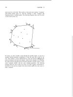
As an example, consider the ring topology shown in Figure 6.14(a) where n = 6.
The entities with the smallest value, 3, will finish waiting before all others: After
6 ×3 = 18 units of time they send a message along the ring. These messages travel
along the ring encountering the other entities while they are still waiting, as shown in
Figure 6.14(b).
IMPORTANT. Protocol Wait solves the minimum-finding problem, not the election:
Unless we assume initial distinct values, more than one entity might have the same
smallest value, and they will all correctly determine that they are the minimum.
362 SYNCHRONOUS COMPUTATIONS
FIGURE 6.14: (a) The time when an entity x would finish waiting; (b) the messages send by
the entities with value 3 at time 6 ×3 = 18 reach the other entities while they are still waiting.
As an example of execution of waiting under the (ID) restriction, consider the ring
topology shown in Figure 6.15 where n = 6, and the values outside the nodes indicate
how long each entity would wait. The unique entity with the smallest value, 3, will
be elected after 6 × 3 = 18 units of time. Its “Stop” message travels along the ring
encountering the other entities while they are still waiting.
FIGURE 6.15: Execution with Initial Distinct Values: a leader is elected.
MIN-FINDING AND ELECTION: WAITING AND GUESSING 363
Protocol Bits Time Notes
Speed
O(n log i) O(2
i

n)
SynchStages
O(n log n) O(i n log n)
Wait
O(n) O(i n) n known
FIGURE 6.16: Waiting yields a more efficient ring election protocol
What is the cost of such a protocol?
Only an entity that becomes minimum originates a message; this message will only
travel along the ring (forwarded by the other entities that become large) until the next
minimum entity. Hence the total number of messages is just n; as these messages are
signals that do not contain any value, we have that Wait uses only O(n) bits. This is
the least amount of transmissions possible ever.
Let us consider the time. It will take f (i
min
,n) = i
min
n time units for the entities
with the smallest value to decide that they are the minima; at most, n −1 additional
time units are needed to notify all others. Hence, the time is O(i,n), where i is
the range of the input values. Compared with the other protocols we have seen for
election in the ring, Speed and SynchStages, the bit complexity is even better (see
Figure 6.16).
Without Simultaneous Initiation We have derived this surprising result assuming
that the entities start simultaneously. If the entities can start at any time, it is possible
that an entity with a large value starts so much before the others that it will finish
waiting before the others and incorrectly determine that it is the minimum.
This problem can be taken care of by making sure that although the entities do
not start at the same time, they will start not too far away (in time) from each other.
To achieve this, it is sufficient to perform a wake-up: When an entity spontaneously
wants to start the protocol, it will first of all send a “Start” message to its neighbor and

then start waiting. An inactive entity will become active upon receiving the “Start”
message, forward it, and start its waiting process.
Let t(x)denote thetimewhen entityx becomesawakeand startsits waiting process;
then, for any two entities x and y,
∀x,y t(y) −t(x) ≤ d(x, y); (6.24)
in particular, no two entities will start more than n −1 clock ticks off from each other.
The waiting function f must now take into account this fact. As before, it is
necessary that if id(x) < id(y), then x must finish waiting before y and its message
should reach y while still waiting; but now this must happen regardless of at what
time t(x) entity x starts and at what time t(y) entity y starts; that is, if id(x) < id(y),
t(x) +f (id(x),n) +d(x,y) <t(y) +f (id(y),n). (6.25)
364 SYNCHRONOUS COMPUTATIONS
As d(x, y) <nfor every two entities in the ring, by Equation 6.24, and by setting
f (0) = 0, it is easy to verify that any function f satisfying the inequality

f (0) = 0
f (v,n) +2n −1 <f(v +1,n)
(6.26)
will make protocol Wait function correctly even if the entities do not start simultane-
ously. Such is, for example, the waiting function
f (v,n) = 2 n v. (6.27)
The cost of the protocol is slightly bigger, but the order of magnitude is the same.
In fact, in terms of bits we are performing also a wake-up that, in a unidirectional
ring, costs n bits. As for the time, the new waiting function is just twice as the old
one; hence, the time costs are at most doubled. In other words, the costs are still those
indicated in Figure 6.16.
In Bidirectional Rings We have considered unidirectional rings. If the ring is bidi-
rectional, the protocol requires marginal modifications, as shown in Figure 6.17. The
same costs as the unidirectional case can be achieved with the same waiting functions.
On the Waiting Function We have assumed that the ring size n is known to the

entities; it is indeed used in the requirements for waiting functions (Expressions 6.22
and 6.26).
An interesting feature (Exercise 6.6.31) is that those requirements would work
even if a quantity
n is used instead of n, provided
n ≥ n. Hence, it is sufficient that
the entities know (the same) upperbound
n on the network size.
If the entities have all available a value
n that is, however, smaller than n, its
use in a waiting function instead of n would in general lead to incorrect results.
There is, however, a range of values for
n that would still guarantee the desired result
(Exercise 6.6.32).
A final interesting observation is the following. Consider the general case when
the entities have available neither n nor a common value
n, that is, each entity only
knows its initial value id(x). In this case, if each entity uses in the waiting function its
value id(x) instead of n, the function would work in some cases, for example, when
all initial values id(x) are not smaller than n. See Exercise 6.6.33.
Universal Waiting Protocol The waiting technique we have designed for rings
is actually much more general and can be applied in any connected network G,
regardless of its topology. It is thus a universal protocol.
The overall structure is as follows:
1. First a reset is performed with message “Start.”
2. As soon as an entity x is active, it starts waiting f (id(x),n) time units.
MIN-FINDING AND ELECTION: WAITING AND GUESSING 365
PROTOCOL Wait

States: S ={ASLEEP, CANDIDATE, LARGE, MINIMUM};

S
INIT
={ASLEEP};
S
TERM
={LARGE, SMALL}.

Restrictions: R ∪ Synch ∪ Ring ∪ Known(n).
ASLEEP
Spontaneously
begin
set alarm:= c(x) +f (id(x),n);
send("Start") to right;
direction := right;
become CANDIDATE;
end
Receiving("Start")
begin
set alarm:= c(x) +f (id(x),n);
send("Start") to other;
direction := other;
become CANDIDATE;
end
CANDIDATE
When(c(x) = alarm)
begin
send("Over") to direction;
become MINIMUM;
end
Receiving("Over")

begin
send("Over") to other;
become LARGE;
end
FIGURE 6.17: Protocol Wait.
3. If, nothing happens while x is waiting, x determines that “I am the minimum”
and initiates a reset with message “Stop.”
4. If, instead, a “Stop” message arrives while x is waiting, then it stops its waiting,
determines that “I am not the minimum” and participates in the reset with
message “Stop.”
Again, regardless of the initiation times, it is necessary that the entities with the
smallest value finish waiting before the entities with larger value and that all those
other entities receive a “Stop” message while still waiting. That is, if id(x) < id(y),
then
t(x) +f (id(x)) +d
G
(x,y) <t(y) +f (id(y)),
366 SYNCHRONOUS COMPUTATIONS
where d
G
(x,y) denotes the distance between x and y in G, and t(x) and t(y) are the
times when x and y start waiting.
Clearly, for all x,y,
|t(x) −t(y)|≤d
G
(x,y);
hence, setting f (0) = 0, we have that any function satisfying

f (0) = 0
f (v) +2d

G
<f(v +1)
(6.28)
makes the protocol correct, where d
G
is the diameter of G. This means that, for
example, the function
f (v) = 2 v (d
G
+1) (6.29)
would work. As n − 1 ≥ d
G
for every G, this also means that the function
f (v) = 2 v n
we had determined for rings actually works in every network; it might not be the most
efficient though (Exercises 6.6.29 and 6.6.30).
Applications of Waiting We will now consider two rather different applications
of protocol Wait. The first is to compute two basic Boolean functions, AND and OR;
the second is to reduce the time costs of protocol Speed that we discussed earlier in
this chapter. In both cases we will consider unidirectional ring for the discussion; the
results, however, trivially generalize to all other networks.
In discussing these applications, we will discover some interesting properties of
the waiting function.
Computing AND and OR Consider the situation where every entity x has a Boolean
value b(x) ∈{0, 1}, and we need to compute the AND of all those values. Assume as
before that the size n of the ring is known. The AND of all the values will be 1 if and
only if ∀xb(x) = 1, that is, all the values are 1; otherwise the result is 0.
Thus, to compute AND it suffices to know if there is at least one entity x with value
b(x) = 0. In other words, we just need to know whether the smallest value is 0or1.
With protocol Waiting we can determine the smallest value. Once this is done, the

entities with such a value know the result. If the result of AND is 1, all the entities
have value 1 and are in state minimum, and thus know the result. If the result of AND
MIN-FINDING AND ELECTION: WAITING AND GUESSING 367
is 0, the entities with value 0 are in state minimum (and thus know the result), while
the others are in state large (and thus know the result).
Notice that if an entity x has value b(x) = 0, using the waiting function of expres-
sion 6.27, its waiting time will be f (b(x)) = 2 b(x) n = 0. That is, if an entity has
value 0, it does not wait at all. To determine the cost of the overall protocol is quite
simple (Exercise 6.6.35).
In a similar way we can use protocol Waiting to compute the OR of the input
values (Exercise 6.6.36).
Reducing Time Costs of Speed The first synchronous election protocol we have
seen for ring networks is Speed, discussed in Section 6.1.4. (NOTE: to solve the
election problemit assumesinitial distinctvalues.)On thebasis ofthe ideaof messages
traveling along the ring at different speeds, this protocol has unfortunately a terrifying
time complexity: exponential in the (a priori unbounded) smallest input value i
min
(see Figure 6.16). Protocol Waiting has a much better complexity, but it requires
knowledge of (an upperbound on) n; on the contrary, protocol Speed requires no such
knowledge.
It is possible to reduce the time costs of Speed substantially by adding Waiting as
a preliminary phase.
As each entity x knows only its value id(x), it will first of all execute Waiting using
2id(x)
2
as the waiting function.
Depending on the relationship between the values and n, the Waiting protocol
might work (Exercise 6.6.33), determining the unique minimum (and hence electing
a leader). If it does not work (a situation that can be easily detected; see Exercise
6.6.34), the entities will then use Speed to elect a leader.

The overall cost of this combine protocol Wait +Speedclearly depends on whether
the initial Waiting succeeds in electing a leader or not.
If Waiting succeeds, we will not execute Speed and the cost will just be O(
i
2
min
)
time and O(n) bits.
If Waiting does not succeed, we must also run Speed that costs O(n) messages
but O(n2
i
min
) time. So the total cost will be O(n) messages and O(i
2
min
+ n2
i
min
) =
O(n2
i
min
) time.However, ifWaitingdoes not succeed,it is guaranteedthat the smallest
initial value is at most n, that is
i
min
<n(see again Exercise 6.6.33). This means that
the overall time cost will be only O(n2
n
).

In other words, whether the initial Waiting succeeds or not, protocol Wait+Speed
will use O(n) messages. As for the time, it will cost either O(
i
2
min
)orO(n2
n
), de-
pending on whether the waiting succeeds or not. Summarizing, using Waiting we can
reduce the time complexity of Speed from O(n2
i
)to
O( Max{
i
2
,n2
n
} )
adding at most O(n) bits.
368 SYNCHRONOUS COMPUTATIONS
Application: Randomized Election If the assumption on the uniqueness of
the identities does not hold, the election problem cannot be solved obviously by any
minimum-finding process, including Wait. Furthermore, we have already seen that
if the nodes have no identities (or, analogously, all have the same identity), then
no deterministic solution exists for the election problem, duly renamed symmetry
breaking problem, regardless of whether the network is synchronous or not. This
impossibility result applies to deterministic protocols, that is, protocols where every
action is composed only of deterministic operations.
A different class of protocols are those where an entity can perform operations
whose result is random, for example, tossing a dice, and where the nature of the ac-

tion depends on outcome of this random event. For example, an entity can toss a coin
and, depending on whether the result is “head” or “tail,” perform a different operation.
These types of protocols will be called randomized; unlike their deterministic coun-
terparts, randomized protocols give no guarantees, either on the correctness of their
result or on the termination of their execution. So, for example, some randomized
protocols always terminate but the solution is correct only with a given probability;
this type of protocols is called Monte Carlo. Other protocols will have the correct
solution if they terminate, but they terminate only with a given probability; this type
of protocols are called Las Vegas.
We will see how protocol Wait can be used to generate a surprisingly simple and
extremely efficient Las Vegas protocol for symmetry breaking. Again we assume that
n is known. We will restrict the description to unidirectional rings; the results can,
however, be generalized to several other topologies (Exercises 6.6.37-6.6.39).
1. The algorithm is composed of a sequence of rounds.
2. In each round, every entity randomly selects an integer between 0 and b as its
identity, where b ≤ n.
3. If the minimum of the chosen values is unique, that entity will become leader;
otherwise, a new round is started.
To make the algorithm work, we need to design a mechanism to find the minimum
and detect if it is unique. But this is exactly what protocol Wait does. In fact, protocol
Wait not only finds the minimum value but also allows an entity x with such a value
to detect if it is the only one. In fact,
–Ifx is the only minimum, its message will come back exactly after n time units;
in this case, x will become leader and send a Terminate message to notify all
other entities.
– If there are more than one minimum, x will receive a message before n time
units; it will then send a “Restart” message and start the next round.
In other words, each round is an execution of protocol Wait; thus, it costs O(n)
bits, including the “Restart” (or “Termination”) messages. The time used by protocol
Wait is O(ni). In our case the values are integers between 0 and b, that is,

i≤ b. Thus,
each round will cost at most O(nb) time.
MIN-FINDING AND ELECTION: WAITING AND GUESSING 369
We have different options with regard to the value b and how the random choice of
the identities is made.For example, wecanset b = n and choose each value with same
probability (Exercise 6.6.40); notice, however, that the larger the b is, the larger the
time costs of each round will be. We will use instead b = 1 (i.e., each entity randomly
chooses either 0 or 1) and employ a biased coin. Specifically, in our protocol, which
we will call Symmetry, we will employ the following criteria:
Random Selection Criteria In each round, every entity selects 0 with probability
1
n
, and 1 with probability
n−1
n
.
Up to now, except for the random selection criteria, there has been little difference
between Symmetry and the deterministic protocols we have seen so far. This is going
to change soon.
Let us compute the number of rounds required by the protocol until termination.
The surprising thing is that this protocol might never terminate, and thus the number
of rounds is potentially infinite.
In fact, with a protocol of type Las Vegas, we know that if it terminates, it solves
the problem, but it might not terminate. This is not a good news for those looking for
protocols with a guaranteed performance. The advantage of this protocol is instead
in the low expected number of rounds before termination.
Let us compute this quantity. Using the random selection criteria described above,
the protocol terminates as soon as exactly one entity chooses 0. For this to happen,
one entity x must choose 0 (this happens with probability
1

n
), while the other n −1
entities mustchoose 1 (thishappenwith probability(
n−1
n
)
n−1
). Asthere are

n
1

= n
choices for x, the probability of exactly one entity chooses 0 is

n
1

1
n
(
n−1
n
)
n−1
= (
n−1
n
)
n−1

.
For n large enough, this quantity is easily bounded; in fact
lim
n→∞

n −1
n

n−1
=
1
e
, (6.30)
where e ≈ 2.7 is thebasis ofthenatural logarithm.This meansthat withprobability
1, protocol Symmetry will terminate after e rounds. In other words,
with probability 1, protocol Symmetry will elect a leader with O(n) bits
in O(n) time.
Obviously, there is no guarantee that a leader will be elected with this cost or will
be elected at all, but with high probability it will and at that cost. This shows the
unique nature of randomized protocols.
370 SYNCHRONOUS COMPUTATIONS
6.3.2 Guessing
Guessing is a technique that allows some entities to determine a value not by trans-
mitting it but by guessing it. Again we will consider the minimum finding and election
problems in ring networks. Let us assume, for the moment, that the ring is unidirec-
tional and that all entities start at the same time (i.e., simultaneous initiation). Let us
further assume that the ring size n is known.
Minimum-Finding as a Guessing Game At the base of the guessing technique
there is a basic utility protocol Decide(p), where p is a parameter available to all
entities. Informally, protocol Decide(p) is as follows:

Decide (p): Every entity x compares its value id(x) with the protocol parameter p.
If id(x) ≤ p, x sends a message; otherwise, it will forward any received message.
There are only two possible situations and outcomes:
S1: All local values are greater than p; in this case, no messages will be trans-
mitted: There will be “silence” in the system.
S2: At least one entity x has id(x) ≤ p ; in this case, every entity will send and
receive a message: There will be “noise” in the system.
The goal of protocol Decide is to make all entities know in which of the two
situations we are. Let us examine how an entity y can determine whether we are in
situation S1orS2. If id(y) ≤ p, then y knows immediately that we are in situation
S2. However, if id(y) >p, then y does not know whether all the entities have values
greater than p (situation S1) or some entities have a value smaller than or equal to p
(situation S2). It does know that if we are in situation S2, it will eventually receive a
message; by contrast, if we are in situation S1, no message will ever arrive.
Clearly, todecide, y must wait; also clearly, it cannot wait forever. How long should
y wait? The answer is simple: If a message was sent by an entity, say x, a message
will arrive at y within at most d(x,y) <ntime units from the time it was sent. Hence,
if y does not receive any message in the first n time units since the start, then none
is coming and we are in situation S1. For this reason, n time units after the entities
(simultaneously) start the execution of protocol Decide(p), all the entities can decide
which situation (S1orS2) has occurred. The full protocol is shown in Figure 6.18.
IMPORTANT. Consider the execution of Decide(p).
– If situation S1 occurs, it means that all the values, including
i
min
= Min{id(x)},
are greater than p, that is, p<
i
min
. We will say that p is an underestimate

on
i
min
.
– If situation S2 occurs, it means that there are some values that are not greater
than
i
min
; thus, p ≥ i
min
. We will say that p is an overestimate on i
min
.
MIN-FINDING AND ELECTION: WAITING AND GUESSING 371
SUBPROTOCOL Decide(p)

Input: positive integer p;

States: S ={START, DECIDED, UNDECIDED};
S
INIT
={START};
S
TERM
={DECIDED}.

Restrictions: R ∪ Synch ∪ Ring ∪ Known(n) ∪ Simultaneous Start.
START
Spontaneously
begin

set alarm:= c(x) +n;
if id(x) ≤ v then
decision:= high;
send("High") to rigth;
become DECIDED;
else
become UNDECIDED;
endif
end
UNDECIDED
Receiving("High")
begin
decision:= high;
send("High") to other;
become DECIDED;
end
When(c(x) = alarm)
begin
decision:= low;
become DECIDED;
end
FIGURE 6.18: SubProtocol Decide(p).
These observations are summarized in Figure 6.19.
NOTE. The condition p =
i
min
is also considered an overestimate.
Using this fact, we can reformulate the minimum-finding problem in terms of a
guessing game:


Each entity is a player. The minimum value
i
min
is a number, previously chosen
and unknown to the player, that must be guessed.

The player can ask question of type “Is the number greater than
p?”
Situation Condition Name Time Bits
S1 p<i
min
“underestimate” n 0
S2 p ≥ i
min
“overestimate” n n
FIGURE 6.19: Results and costs of executing protocol Decide.
372 SYNCHRONOUS COMPUTATIONS

Each question corresponds to a simultaneous execution of Decide(p). Situa-
tions S1 and S2 correspond to a "YES" and a "NO" answer to the question,
respectively.
A guessing protocol will just specify which questions should be asked to discover
i
min
. Initially, all entities choose the same initial guess p
1
and simultaneously perform
Decide(p
1
). Aftern timeunits,allentitieswill beawareofwhetheror noti

min
is greater
than p
1
(situation S1 and situation S2, respectively). On the basis of the outcome,
a new guess p
2
will be chosen by all entities that will then simultaneously perform
Decide(p
2
). In general, on the basis of the outcome of the execution of Decide(p
i
),
all entities will choose a new guess p
i+1
. The process is repeated until the minimum
value
i
min
is unambiguously determined.
Depending on which strategy is employed for choosing p
i+1
given the outcome
of Decide(p
i
), different minimum-finding algorithms will result from this technique.
Before examining how to best play (and win) the game, let us discuss the costs of
asking a question, that is, of executing protocol Decide.
Observe that the number of bits transmitted when executing Decide depends on the
situation, S1orS2, we are in. In fact in situation S1, no messages will be transmitted

at all. By contrast, in situation S2, there will be exactly n messages; as the content
of these messages is not important, they can just be single bits. Summarizing, If our
guess is an overestimate, we will pay n bits; if it is an underestimate, it will cost
nothing.
As for the time costs, each execution of Decide will cost n time units regardless of
whether it is an underestimate or overestimate.
This means that we pay n time units for each question; however, we pay n bits
only if our guess is an overestimate. See Figure 6.19.
Our goal must, thus, be to discover the number, asking few questions (to minimize
time) of which as few as possible are overestimates (to minimize transmission costs).
As we will see, we will unfortunately have to trade off one cost for the other.
We will first consider a simplified version of the game, in which we know an
upperbound M on the number to be guessed, that is, we know that i
min
∈ [1,M] (see
Figure 6.20). We will then see how to easily and efficiently establish such a bound.
Playing the Game We will now investigate how to design a successful strategy
for the guessing game. The number
i
min
to be guessed is known to be in the interval
[1,M] (see Figure 6.20).
Let us denote by q the number of questions and by k ≤ q the number of overes-
timates used to solve the game; this will correspond to a minimum-finding protocol
that uses qntime and kn bits.Aseachoverestimate costs us n bits, to design an overall
FIGURE 6.20: Guessing in an interval.