Orr, F. M. - Theory of Gas Injection Processes Episode 4 pot
Bạn đang xem bản rút gọn của tài liệu. Xem và tải ngay bản đầy đủ của tài liệu tại đây (230.5 KB, 20 trang )
4.2. SHOCKS 51
C
i
=C
i
Ι
C
i
=C
i
Π
ξξ+∆ξ
shock at τ shock at τ+∆τ
Figure 4.6: Motion of a shock.
original conservation equation. In other words, it is a statement that volume is conserved across
the shock, just as Eq. 4.1.1 states that volume is conserved at locations where all the derivatives
exist. Eq. 4.2.2 says that the velocity at which the shock propagates is set by the slope of a line
that connects the two states on either side of the shock on a plot of F
1
against C
1
such as that
showninFig.4.1.
Now we apply the jump condition to determine what happens at the leading edge of the dis-
placement zone, where fast characteristics (the characteristics in Fig. 4.5 that have high values of
dF
1
/dS
1
) intersect the characteristics for the initial composition. Point a in Fig. 4.7 is the initial
composition, which is the composition on the downstream side of the leading shock, and points b,
c, d, e, f,andg are possible composition points for the fluid on the upstream side of the shock. Any
of the shock constructions shown in Fig. 4.7 satisfies Eq. 4.2.2. Hence some additional reasoning is
required to select which shock is part of a unique solution to the flow problem.
Two physical ideas play a role in that reasoning. The first is simply an observation that
compositions that make up the downstream portion of the solution must have moved more rapidly
than compositions that lie closer to the inlet. If not, slow-moving downstream compositions would
be overtaken by faster compositions upstream. The idea is frequently stated [31] as a
Velocity Constraint: Wave velocities in the two-phase region must decrease monoton-
ically for zones in which compositions vary continuously as the solution composition
path is traced from downstream compositions to upstream compositions .
When the velocity constraint is satisfied, the solution will be single-valued throughout. Composition
variations that satisfy the velocity constraint are sometimes described as compatible waves,andthe
velocity constraint may also be called a compatibility condition.
The second idea is that a shock can exist only if it is stable in the sense that it would form
again if it were somehow smeared slightly from a sharp jump, as might happen if a small amount of
physical dispersion were present, for example. That idea can be stated in terms of wave velocities
[67, 83, 106] as an
Entropy Condition: Wave velocities on the upstream side of the shock must be greater
52 CHAPTER 4. TWO-COMPONENT GAS/OIL DISPLACEMENT
than (or equal to) the shock velocity and wave velocities on the downstream side must
be less than (or equal to) the shock velocity. (In the examples considered here, the wave
velocity can be equal to the shock velocity on only one side of the shock at a time.)
For the application considered here, the condition really has nothing to do with the thermodynamic
entropy function, but the name has been universally used in descriptions of solutions to hyperbolic
conservation laws since the ideas behind entropy conditions were first derived for compressible
fluid flow problems in which entropy must increase across the shock. Consider what would happen
to a shock that was slightly smeared if the entropy condition were not satisfied. Slow-moving
compositions upstream of the shock would be left behind by fast-moving compositions downstream
of the shock, and as a result, the shock would pull itself apart. Hence, the entropy condition must
be satisfied if a shock is to be stable. A shock that does satisfy the entropy condition is said to
be self-sharpening. For a detailed discussion of the various mathematical forms in which entropy
conditions can be expressed, see the review given by Rhee, Aris and Amundson [106, pp. 213–220
and pp. 341–348].
We now apply the velocity constraint and the entropy condition to obtain a unique solution for
two-component displacement. Fig. 4.8 illustrates possible solutions for the leading shocks indicated
in Fig. 4.7. Consider, for example, a shock that connects downstream composition a and upstream
composition b. The top left panel of Fig. 4.8 shows the location of the shock at some fixed time and
also shows how the solution would behave if the concentration of C
1
increased smoothly upstream
of the shock. The wave velocity, Λ, of the shock (Eq. 4.2.2) is given by the slope of the chord that
connects points a and b on Fig. 4.7. That velocity is clearly less than one, and hence the a→b
shock moves more slowly than the single-phase compositions downstream of the shock, which have
unit velocity. The wave velocity of the composition just upstream of the shock is given by dF
1
/dC
1
at point b. That velocity is lower still than the wave velocity of the shock. Thus, the a→b shock
violates the entropy condition. As the C
1
concentration upstream of the shock increases, however,
the wave velocities increase to values greater than the shock velocity, a variation that produces
compositions that violate the velocity constraint. Hence, a solution that includes a shock from a
to b followed by a continuously varying composition violates both the velocity constraint and the
entropy condition and can be ruled out, therefore.
The a→c, a→d,anda→e shocks all satisfy the entropy condition, but all three violate the
velocity constraint, as the profiles in Fig. 4.8 show. The a→g satisfies the velocity constraint, but
it violates the entropy condition because the wave velocity of the upstream composition is lower
than the shock velocity. Hence, the only remaining possible solution is that shown for the a→f
shock.
The point f is the point at which the chord drawn from point a is tangent to the overall fractional
flow curve. The a→f shock does satisfy the entropy condition, but it does so in a special way. The
wave velocity of the composition C
1
of point f is equal to the shock velocity, because the shock
velocity is given by the slope of the tangent a–f, and that chord slope is the same as dF
1
/dC
1
at
point f. A shock in which the shock velocity equals the wave velocity on one side of the shock is
sometimes called a semishock [106, pp. 217–219] , an intermediate discontinuity [40], or a tangent
shock [82]. Because the leading shock must be a semishock if it is to satisfy the velocity constraint
and the entropy condition, the composition of the fluid on the upstream side of the shock can be
found easily by solving
4.2. SHOCKS 53
0.0
0.2
0.4
0.6
0.8
1.0
Overall Fractional Flow of Component 1, F
1
0.0
0.2
0.4 0.6 0.8 1.0
Overall Volume Fraction of Component 1, C
1
a
b
c
d
e
f
g
Figure 4.7: Possible shocks from the initial state at point a.
dF
1
dC
1
|
II
=
F
II
i
− F
I
i
C
II
i
− C
I
i
. (4.2.3)
The tangent construction described in Eq. 4.2.3 and shown in Fig. 4.7 is equivalent to the well-
known Welge tangent construction [133] used to solve the problem of Buckley and Leverett [10] for
water displacing oil.
Just as a shock was required in order to make the solution single-valued at the leading edge of
the transition zone, another shock is required at the trailing edge. The characteristics in Fig. 4.4
for the injection composition intersect the characteristics in Fig. 4.5 for slow moving compositions,
C
1
, greater than the shock composition. Reasoning similar to that for the leading shock shows that
the trailing shock also is a semishock, this time with the wave velocity on the downstream side of
the shock equal to the shock velocity. In fact, similar arguments indicate that a shock must form
any time the number of phases changes for the fractional flow relation used here.
Fig. 4.9 shows the resulting tangent constructions for the leading (a→b) and trailing shock
(c→d). Fig. 4.10 gives the completed solution profiles of S
1
and C
1
. Each profile includes a zone of
constant state with the initial composition ahead of the leading shock, a zone of continuous variation
of overall composition and saturation between the leading shock and the trailing shock, and finally
another zone of constant state with the injection composition behind the trailing shock. The
solution in Fig. 4.10 is reported as a function of ξ/τ, which is the wave velocity of the corresponding
54 CHAPTER 4. TWO-COMPONENT GAS/OIL DISPLACEMENT
0
1
C
1
01
ξ
a-b
0
1
C
1
01
ξ
a-c
0
1
C
1
01
ξ
a-d
0
1
01
ξ
a-e
0
1
01
ξ
a-f
0
1
01
ξ
a-g
Figure 4.8: Composition profiles for the leading shocks to various two-phase compositions.
value of C
1
. In this homogeneous, quasilinear problem, the wave velocity of any composition is
constant, and hence the position of any composition that originated at the inlet must be a function
of ξ/τ only. In fact, Lax [67] showed that the solution to a quasilinear Riemann problem is always
a function of ξ/τ only. The spatial position of a given composition C
1
can be obtained simply by
multiplying the corresponding value of ξ/τ by the value of τ at which the solution is desired.
Another version of the solution is shown in Fig. 4.11, which includes a τ-ξ diagram and a plot
of the C
1
profile at τ =0.60. Shown in the τ-ξ portion of Fig. 4.11 are the trajectories of the
leading and trailing shocks and a few of the characteristics. The locations, ξ,oftheshocksand
the compositions associated with specific characteristics can be read directly from the t-x diagram
for a particular value of τ, as Fig. 4.11 illustrates. From Fig. 4.11 it is easy to see that as the flow
proceeds, the solution retains the shape shown in the profiles of Figs. 4.10 and 4.11, but the entire
solution stretches as fast-moving compositions pull away from slow-moving ones. That behavior is
typical of problems in which convective phenomena dominate the transport.
Fig. 4.11 also illustrates the point that when the entropy condition is satisfied for a particular
4.2. SHOCKS 55
0.0
0.2
0.4
0.6
0.8
1.0
Overall Fractional Flow of Component 1, F
1
0.0
0.2
0.4 0.6 0.8 1.0
Overall Volume Fraction of Component 1, C
1
a
b
c
d
Figure 4.9: Leading and trailing shock constructions.
shock, characteristics on either side of the trajectory of a shock either impinge on the shock trajec-
tory or are at least parallel to the shock trajectory. In the case of the leading shock, for example,
the characteristics of the initial composition, which lies downstream of the shock, intersect the
shock trajectory, while characteristic just upstream of the shock overlaps the shock trajectory. The
reverse is true at the trailing shock.
Between the trajectories of the shocks is the fan of characteristics associated with the continuous
variation of composition, which is known as a spreading wave,ararefaction wave,oranexpansion
wave. Because the characteristics all emanate from a single point, the origin, they are also referred
to as a centered wave. The change in slope of the characteristics in the spreading wave reflects
the fact that the slope of the fractional flow curve drops rapidly over a fairly narrow range of
composition (see Fig. 4.2). As a result, the wave velocity declines significantly during the relatively
small composition change between the leading and trailing shocks. In the solution shown in Fig. 4.10
the overall compositions and saturations vary in the two-phase region, but the phase compositions
do not. They are fixed by the specified phase equilibrium. It is the differing amounts of the two
phases present and flowing that change the overall composition and fractional flow.
56 CHAPTER 4. TWO-COMPONENT GAS/OIL DISPLACEMENT
0.0
0.5
1.0
C
1
0.0 0.5 1.0 1.5
ξ/τ
a
b
c
d
0.0
0.5
1.0
S
1
0.0 0.5 1.0 1.5
ξ/τ
a
b
c
d
Figure 4.10: Solution composition and saturation profiles.
4.3 Variations in Initial or Injection Composition
In the binary gas/oil displacement problem, the leading shock forms because some two-phase mix-
tures of injected fluid with initial fluid move rapidly and overtake the initial composition. The
trailing shock forms because some Component 2 can evaporate into the unsaturated injected vapor.
How fast the leading and trailing shocks move depends on the initial and injection compositions. In
this section we examine briefly the sensitivity of the solution to the binary displacement problem
to changes in the initial and injection compositions.
Fig. 4.12 shows a set of key points on the fractional flow curve. Points a, b, c,andd are from
the solution discussed in the previous section. Points a and d are the initial and injection values,
and points b and c are the tangent points for the leading and trailing semishocks. Point e is the
saturated vapor phase, and point i is the saturated liquid. Point f corresponds to S
1
=1−S
or
,and
point h is that at which S
1
= S
gc
.Pointg is the intersection of the F
1
= C
1
line with the overall
fractional flow curve. Point j is the inflection point in the fractional flow curve. It corresponds to
the maximum in dF
1
/dC
1
showninFig.4.2.
Fig. 4.13 shows examples of the solutions that result when the initial composition is fixed at
C
a
1
and the injection composition is varied. The six panels in Fig. 4.13 illustrate changes in the
appearance of the composition profiles for injection compositions with decreasing volume fractions,
C
inj
1
. Fig. 4.14 shows the corresponding characteristic (τ-ξ) diagrams. The following observations
can be made for injection compositions in the regions bounded by the key points in Fig. 4.13:
dtoe: For injection compositions in the range 1 >C
inj
1
>C
e
1
, the solution still
4.3. VARIAT IONS IN INITIAL OR INJECTION COMPOSITION 57
0.0
0.5
1.0
C
1
0.0 0.5 1.0
ξ
0.0
0.2
0.4
0.6
0.8
1.0
τ
0 1
Trailing Shock
Leading
Shock
C
1
= 0.68
C
1
= 0.71
0
0.0 0.5 1.0
Figure 4.11: Evaluation of the solution at a specific time, τ,fromtheτ-ξ diagram.
includes leading and trailing semishocks connected by a spreading wave (see the top
left panel of Fig. 4.13), and the τ-ξ diagram shown in the corresponding panel in Fig.
4.14 is qualitatively similar to Fig. 4.11. As C
inj
1
is decreased, the trailing shock speed
decreases, reaching zero when the injected fluid is vapor saturated with component 2
(C
inj
1
= C
e
1
). The leading portion of the solution is unchanged, however.
etof:Compositions in the range C
e
1
>C
inj
1
>C
f
1
have zero wave velocity because
dF
1
/dC
1
= 0. There is a trailing shock from the injection composition to C
e
1
, but it has
zero wave velocity, and hence the fan of characteristics in Fig. 4.14 extends all the way
to the ξ = 0 axis. The leading portion of the solution remains unchanged.
ftob:An injection composition between f and b has nonzero wave velocity, and as a
result, the solution in the lower left panel of Fig. 4.13 shows a zone of injection composi-
tions at the upstream end that all propagate with the same wave velocity. That portion
of the solution has a set of parallel characteristics in Fig. 4.14 that emanate from the
ξ = 0 axis. The fan of characteristics that represents the spreading wave terminates at
the characteristic that represents that propagation of the injection composition. When
C
inj
1
= C
b
1
, the entire solution upstream of the leading shock is that zone of constant
58 CHAPTER 4. TWO-COMPONENT GAS/OIL DISPLACEMENT
0.0
0.2
0.4
0.6
0.8
1.0
Overall Fractional Flow of Component 1, F
1
0.0
0.2
0.4 0.6 0.8 1.0
Overall Volume Fraction of Component 1, C
1
a
i
h
g
j
fe
d
b
c
Figure 4.12: Composition ranges for variation of injection and initial compositions.
composition with C
1
= C
b
1
. The leading shock velocity is still unchanged, however.
btog:A leading semishock is no longer possible for C
b
1
>C
inj
1
>C
g
1
, because contin-
uous variation from the tangent shock point to the injection composition is prohibited
by the velocity rule. A leading shock to the injection composition followed by a set of
constant compositions at the injection composition satisfies the entropy condition and
velocity constraint. The top right panel in Fig. 4.14 indicates, for example, that the
characteristics associated with the injection composition intersect the leading shock tra-
jectory, as do the characteristics associated with the initial composition, an indication
that the entropy condition is satisfied. The leading shock velocity is given by Eq. 4.2.2
with the known compositions C
init
1
and C
inj
1
. The leading shock velocity is now lower
than that of the leading semishocks that form for C
inj
1
>C
b
1
.WhenC
inj
1
= C
g
1
,the
leading shock has unit velocity.
gtoh: A leading shock directly from the injection composition to the initial com-
position is no longer possible because it would violate the entropy condition. A shock
from the initial composition to the injection composition would have a velocity less than
one. The characteristics of the initial composition (see the middle right panel of Fig.
4.14)would not intersect the shock trajectory, and hence, the entropy condition would
not be satisfied. The only path available that does not violate the entropy condition is
4.3. VARIAT IONS IN INITIAL OR INJECTION COMPOSITION 59
0
1
C
1
01
ξ
d-e
C
1
inj
=0.975
0
1
C
1
01
ξ
e-f
C
1
inj
=0.920
0
1
C
1
01
ξ
f-b
C
1
inj
=0.770
0
1
01
ξ
b-g
C
1
inj
=0.560
0
1
01
ξ
g-h
C
1
inj
=0.320
0
1
01
ξ
h-i
C
1
inj
=0.215
Figure 4.13: Effect of changes in injection composition.
a leading shock with unit velocity to the saturated liquid composition, C
i
1
, followed by
a slower trailing shock to the injection composition. The characteristics of the injection
composition intersect the trailing shock, and the characteristics of the initial composi-
tion intersect the leading shock. The zone between the two shocks is what is known as
a zone of constant state. The composition i has two wave velocities: one is the leading
shock velocity, and the other is the trailing shock velocity.
htoi: Thesituationisthesameasforg-h, except that the trailing shock has zero
velocity. The trailing shock is a jump from the injection composition to the saturated
liquid composition, C
i
1
.
Fig. 4.13 indicates that the form of the solution changes significantly as the injection composition
changes. Solution behavior also changes if the initial composition is changed. Fig. 4.15 illustrates
what happens if the injection composition is fixed at C
inj
1
= C
d
1
= 1, and the initial composition
is varied in ranges bounded by the key points shown in Fig. 4.12. Four composition intervals are
60 CHAPTER 4. TWO-COMPONENT GAS/OIL DISPLACEMENT
0
1
τ
0 1
d-e
0
1
τ
0 1
e-f
0
1
τ
0 1
ξ
f-b
0
1
0 1
b-g
0
1
0 1
g-h
0
1
0 1
ξ
h-i
Figure 4.14: τ-ξ diagrams for displacements illustrated in Fig. 4.13.
important:
atoi:As the amount of component 1 in the initial mixture increases, the velocity of
the leading semishock also increases slightly (the slope of the tangent drawn from the
initial composition to the fractional flow curve increases), and the composition on the
upstream side of the leading shock decreases slightly below point b. The remainder of
the composition profile upstream of the leading shock is unaffected.
itoj: Increasing C
1
from i toward j causes the leading shock speed to increase sub-
stantially and the shock composition to approach j.
jtoc:For C
init
1
greater than the inflection composition, there is no leading shock. The
leading portion of the solution is simply a spreading wave.
ctoe: When C
init
1
>C
c
1
, the trailing shock is no longer a semishock. Instead that
evaporation shock is what is known as a genuine shock, a jump from C
init
1
to C
inj
1
,with
4.4. VOLUME CHANGE 61
0
1
C
1
01
ξ
a-i
C
1
init
=0.18
0
1
C
1
01
ξ
i-j
C
1
init
=0.30
0
1
01
ξ
j-c
C
1
init
=0.62
0
1
01
ξ
c-e
C
1
init
=0.80
Figure 4.15: Effect of changes in initial composition.
velocity given by Eq. 4.2.2. The trailing shock velocity increases as C
init
1
is increased,
reaching unit velocity when C
init
1
= C
e
1
.
Figs. 4.13 and 4.15 indicate that solutions for binary gas/oil displacement show considerable
variation as the injection and initial conditions are changed. Many of the features of these binary
solutions reappear in the multicomponent solutions that are considered in subsequent chapters,
and hence a detailed understanding of the binary solutions is useful underpinning for the analysis
of more complex multicomponent flows.
4.4 Volume Change
When components change volume as they transfer from one phase to another, volume is not con-
served, and the appropriate balance equation on moles of component i is Eq. 2.3.9 written for the
two components,
∂G
1
∂τ
+
∂H
1
∂ξ
=0, (4.4.1)
∂G
2
∂τ
+
∂H
2
∂ξ
=0, (4.4.2)
where
G
i
= x
i1
ρ
1D
S
1
+ x
i2
ρ
2D
(1 − S
1
), (4.4.3)
62 CHAPTER 4. TWO-COMPONENT GAS/OIL DISPLACEMENT
H
i
= v
D
(x
i1
ρ
1D
f
1
+ x
i2
ρ
2D
(1 − f
1
)). (4.4.4)
4.4.1 Flow Velocity
The local flow velocity, v
D
, appears in both balance equations in the definition of H
i
.Thatvelocity
changes when components change volume as they transfer between phases or as the composition of a
phase changes. When compositions change along a tie line, however, the local flow velocity remains
constant [22]. When a composition variation remains on a single tie line within the two-phase
region (as it must for this binary problem where there is only one tie line), the phase composition,
x
i1
and x
i2
, and the dimensionless molar phase densities, ρ
1D
and ρ
2D
, remain constant at the
values for the equilibrium phases. As a result, substitution of the definitions for G
i
and H
i
(Eqs.
4.4.3 and 4.4.4) into Eqs. 4.4.1 and 4.4.2 followed by rearrangement gives
∂S
1
∂τ
+
∂
∂ξ
v
D
f
1
+
x
12
ρ
2D
x
11
ρ
1D
−x
12
ρ
2D
=0, (4.4.5)
and
∂S
1
∂τ
+
∂
∂ξ
v
D
f
1
+
x
22
ρ
2D
x
21
ρ
1D
−x
22
ρ
2D
=0. (4.4.6)
Subtraction of Eq. 4.4.6 from Eq. 4.4.5 yields an expression for the spatial derivative of the velocity,
x
12
ρ
2D
x
11
ρ
1D
− x
12
ρ
2D
−
x
22
ρ
2D
x
21
ρ
1D
− x
22
ρ
2D
∂v
D
∂ξ
=0. (4.4.7)
It is convenient to rewrite Eq. 4.4.7 in terms of the equilibrium K-values, x
11
= K
1
x
12
and x
21
=
K
2
x
22
,whichgives
ρ
2D
K
1
ρ
1D
−ρ
2D
−
ρ
2D
K
2
ρ
1D
− ρ
2D
∂v
D
∂ξ
=0. (4.4.8)
As long as K
1
= K
2
, which must be true if two phases are to form, Eq. 4.4.8 shows that
∂v
D
∂ξ
=0.
Hence, the local flow velocity is constant for composition variations in the two-phase region along
a single tie line. This behavior results from the fact that the phase densities remain constant for
mixtures on a single tie line in the two-phase region.
4.4.2 Characteristic Equations
The characteristic equations can now be obtained just as they were in Section 4.1. Arguments
similar to those given in Section 4.1 indicate that H
1
is a function of G
1
only, and hence,
∂G
1
∂τ
+
dH
1
dG
1
∂G
1
∂ξ
=0. (4.4.9)
G
1
is a function of ξ and τ, and therefore,
dG
1
dη
=
∂G
1
∂τ
dτ
dη
+
∂G
1
∂ξ
dξ
dη
. (4.4.10)
Comparison of Eqs. 4.4.9 and 4.4.10 gives the characteristic equations,
4.4. VOLUME CHANGE 63
dG
1
dη
=0, (4.4.11)
dτ
dη
=1, (4.4.12)
dξ
dη
=
dH
1
dG
1
. (4.4.13)
Comparison of Eqs. 4.4.11–4.4.13 with the corresponding equations for constant volume flow,
Eqs. 4.1.9–4.1.11, indicates that within the two-phase region, at least, the solutions for flow with
and without volume change have similar structure. The similarity can be seen more clearly if
dH
1
/dG
1
is evaluated. Differentiation of Eq. 4.4.4 gives
dH
1
dG
1
= v
D
(x
11
ρ
1D
− x
12
ρ
2D
)
df
1
dG
1
. (4.4.14)
Eq. 4.4.3 can be rearranged to show that S
1
is a function of G
1
only, and therefore,
df
1
dG
1
=
df
1
dS
1
dS
1
dG
1
=
1
x
11
ρ
1D
−x
12
ρ
2D
df
1
dS
1
. (4.4.15)
Substitution of Eq. 4.4.15 into Eq. 4.4.14 shows that
dH
1
dG
1
= v
D
df
1
dS
1
. (4.4.16)
Hence for compositions within the two-phase region, the wave velocity is simply the wave velocity
for constant volume flow scaled by the appropriate local flow velocity within the two-phase region.
The distinction between flow velocity and wave velocity is an important one . The flow velocity
is the total volumetric flow rate of all the phases per unit area. The wave velocity is the speed at
which a given composition propagates. The two are very different. When volume is not conserved,
the flow velocity does not change when the composition varies along a single tie line, but it does
change at shocks that enter or leave the two-phase region. Hence, the next step is to determine
how flow velocity varies across the shocks.
4.4.3 Shocks
Consider the trailing shock from the injection composition, G
d
1
, to composition, G
c
1
, in the two-phase
region. A shock balance indicates that the shock wave velocity, Λ
cd
,isgivenby
Λ
cd
=
H
c
i
− H
d
i
G
c
i
− G
d
i
,i=1, 2. (4.4.17)
Eqs. 4.4.17 can be written for either component. When volume is not conserved, the two
equations are independent. As a result, the shock balances can be solved for both the downstream
composition, G
c
i
,andtheflowvelocity,v
c
D
. To show how that is done, it is convenient to write
H
i
= v
D
α
i
= v
D
n
p
j=1
x
ij
ρ
jD
f
j
. (4.4.18)
64 CHAPTER 4. TWO-COMPONENT GAS/OIL DISPLACEMENT
To find v
c
D
, we write Eqs. 4.4.17 for components 1 and 2 and eliminate Λ
cd
,whichgives
v
d
D
α
d
1
− v
c
D
α
c
1
G
d
1
−G
c
1
=
v
d
D
α
d
2
−v
c
D
α
c
2
G
d
2
−G
c
2
. (4.4.19)
v
d
D
is the injection flow velocity, and by definition (Eq. 2.3.2), v
d
D
=1. α
d
1
and G
d
1
are the injection
data, so Eq. 4.4.19 can be solved for v
c
D
once G
c
2
and α
c
2
are determined,
v
c
D
=
α
d
2
(G
d
1
−G
c
1
) − α
d
1
(G
d
2
−G
c
2
)
α
c
2
(G
d
1
−G
c
1
) − α
c
1
(G
d
2
− G
c
2
)
. (4.4.20)
Application of the entropy condition and velocity constraint shows that if injection composition
is single-phase vapor, the trailing shock is a semishock that satisfies
v
c
D
df
1
dS
1
=
α
d
i
−v
c
D
α
c
i
G
d
i
−G
c
i
,i=1or 2. (4.4.21)
When component 2 is not present in the injection fluid, v
c
D
can be eliminated from Eq. 4.4.21, and
it can then be solved to find the composition at point c. Otherwise, Eqs. 4.4.20 and 4.4.21 can be
solved simultaneously for v
c
D
and point c.
Similar manipulations give expressions that can be solved for the composition at the leading
shock, G
b
i
,andtheflowvelocity,v
a
D
, ahead of the shock. The wave velocity of the leading shock is
Λ
ab
=
H
a
i
−H
b
i
G
a
i
−G
b
i
, (4.4.22)
where G
a
i
and H
a
i
are the initial values. For an initial composition in the single-phase region, the
leading shock is a semishock determined by
v
a
D
v
c
D
=
α
b
1
(G
a
2
−G
b
2
) − α
b
2
(G
a
1
−G
b
1
)
α
a
1
(G
a
2
−G
b
2
) − α
a
2
(G
a
1
− G
b
1
)
, (4.4.23)
and
df
1
dS
1
=
α
a
i
(v
a
D
/v
b
D
) − α
b
i
G
a
i
− G
b
i
,i=1or 2. (4.4.24)
Therefore, when v
b
D
is known, as it is from the solution for the trailing shock because v
b
D
= v
c
D
,
v
a
D
and G
b
i
can be obtained by solving Eqs. 4.4.23 and 4.4.24. Thus, in a binary displacement,
only three flow velocities exist: the known injection velocity behind the trailing shock, a fixed flow
velocity in the two-phase region, and a different flow velocity ahead of the leading shock.
4.4.4 Example Solution
To illustrate how volume change affects flow behavior, we consider displacement of a hydrocarbon,
decane (C
10
), by a gas, carbon dioxide (CO
2
), at 500 psia (34 atm) and 160 F (71 C). Table 4.1
reports Peng-Robinson equilibrium phase compositions and the initial, injection and phase molar
densities. Table 4.2 gives compositions, wave velocities, and flow velocities for the solution with
volume change, and Table 4.3 reports the corresponding values for the solution without volume
change. In both cases, the fractional flow curves were assumed to be Eqs. 4.1.20-4.1.22, with
4.4. VOLUME CHANGE 65
Table 4.1: Equilibrium Phase Compositions and Fluid Properties at 500 psia (34 atm) and 160 F
(71 C)
Fluid x
CO
2
x
C
10
ρ ρ µ
(gmol/l) (g/cm
3
) (cp)
Initial Oil 0. 1. 4.829 0.6869 -
Equil. Liq. 0.2733 0.7267 5.988 0.6910 0.333
Equil. Vap. 0.9976 0.0024 1.378 0.0610 0.018
Injected Gas 1. 0. 1.375 0.0605 -
S
or
= S
gc
= 0. Overall mole fractions shown in Table 4.2 were calculated from the values of G
i
by
noting that
z
i
=
G
i
n
p
j=1
ρ
jD
S
j
. (4.4.25)
Overall compositions in Table 4.3 were calculated from volume fractions using the pure component
densities in Table 4.1 according to
z
i
=
ρ
ci
{c
i1
S
1
+ c
i2
(1 − S
1
)}
S
1
n
c
i=1
ρ
ci
c
i1
+(1− S
1
)
n
c
i=1
ρ
ci
c
i2
, (4.4.26)
where the phase volume fractions are given by Eq. 2.4.1 with the phase mole fraction data in Table
4.1.
Fig. 4.16 and the wave velocity (dξ/dτ) data in Tables 4.2 and 4.3 show that the composition
profiles have similar appearances in the displacements with and without volume change, but the
flow proceeds more slowly when volume is not constant. In particular, the velocity of the leading
shock is much lower when effects of volume change are included. In fact, it has a wave velocity less
than one, which means that more than one pore volume must be injected for the leading shock to
reach the outlet (at ξ = 1) when volume is variable. The change in flow velocity occurs because
CO
2
occupies much less volume when it is dissolved in the liquid phase than it does in the vapor
phase [19]. When CO
2
saturates the C
10
present in the two-phase region, therefore, significant
volume is lost, and the flow slows accordingly. As Table 4.2 and Fig. 4.16 show, the flow velocity,
v
D
, ahead of the leading shock is only about half the injection velocity.
In both displacements there is a slow-moving trailing evaporation shock. It moves slowly because
the solubility of C
10
in CO
2
is small. In other words, a large amount of CO
2
must be injected to
evaporate the remaining C
10
. The velocity change at the trailing shock is small, however. The
concentration of C
10
in the vapor phase is so low that the volume change associated with the
transfer of C
10
to the vapor has minimal effect on the flow velocity. The values of v
D
in Table 4.2
indicate again that v
D
remains constant for compositions in the two-phase region.
The wave velocities in Fig. 4.16 and Tables 4.2 and 4.3 also indicate that the displacement
of C
10
by CO
2
is relatively inefficient. While the leading shock moves with appreciable velocity,
66 CHAPTER 4. TWO-COMPONENT GAS/OIL DISPLACEMENT
0.0
0.5
1.0
z
1
0.0 0.5 1.0 1.5
ξ/τ
aa
b
b
c
c
d
No volume change
Volume change
0.0
0.5
1.0
S
1
0.0 0.5 1.0 1.5
ξ/τ
0.0
0.5
1.0
v
D
0.0 0.5 1.0 1.5
ξ/τ
Figure 4.16: Displacement of C
10
by CO
2
, with and without volume change as components transfer
between phases.
4.5. COMPONENT RECOVERY 67
Table 4.2: Displacement of C
10
by CO
2
with Volume Change
Label z
CO
2
S
1
dξ
dτ
v
D
τ R
C
10
a 0.0000 0.0000 0.5097 0.5097 < 1.0932 -
b 0.3676 0.3941 0.9147 0.9999 1.0932 0.5574
- 0.4088 0.5000 0.3710 0.9999 2.6956 0.6503
- 0.5264 0.7000 0.0662 0.9999 15.097 0.8087
c 0.7020 0.8630 0.0063 0.9999 158.75 1.0000
d 1.0000 1.0000 1.0000 1.0000 > 158.75 1.0000
Table 4.3: Displacement of C
10
by CO
2
without Volume Change
Label z
CO
2
S
1
dξ
dτ
v
D
τ Q
C
10
a 0.0000 0.0000 1.0000 1.0000 < 0.7712 -
b 0.7214 0.3539 1.2967 1.0000 0.7712 0.7712
- 0.7842 0.5000 0.3710 1.0000 2.6954 0.8336
- 0.8703 0.7000 0.0662 1.0000 15.096 0.9137
c 0.9294 0.8375 0.0118 1.0000 85.092 1.0000
d 1.0000 1.0000 1.0000 1.0000 > 85.092 1.0000
somewhat higher CO
2
concentrations (and saturations) move much more slowly. As a result, C
10
is recovered much more slowly after the arrival of the leading shock at the outlet.
4.5 Component Recovery
The amount of component i recovered at the outlet can be calculated from the composition and
saturation profiles obtained as part of the solution to the Riemann problem. Just as the spatial
distribution of compositions is found by solving a differential material balance, the recovery of
individual components is obtained from an integral balance over the flow length. The amount of
any component recovered from the porous medium is simply the amount present initially plus the
amount of that component injected during the time the flow has taken place minus the amount of
that component currently present in the porous medium. When volume change is neglected, for
a porous medium of dimensionless length ξ = 1, the resulting expression for Q
1
,thevolumeof
component 1 recovered, is
Q
1
= C
init
1
+ F
inj
1
τ −
1
0
C
1
dξ. (4.5.1)
Prior to the arrival of the leading shock, fluid leaves the porous medium with the fractional flow
of the initial mixture. Because the initial composition is constant, the recovery of each component
is just τF
init
i
. Breakthrough of injected fluid occurs at τ
BT
, when the leading shock arrives at the
outlet, where ξ = 1. Accordingly,
68 CHAPTER 4. TWO-COMPONENT GAS/OIL DISPLACEMENT
τ
BT
=
1
Λ
ab
. (4.5.2)
After breakthrough, the integral in Eq. 4.5.1 can be evaluated as
1
0
C
1
dξ =
τ Λ
cd
0
C
1
dξ +
1
τ Λ
cd
C
1
dξ (4.5.3)
= C
inj
1
Λ
cd
τ +
1
τ Λ
cd
C
1
dξ. (4.5.4)
The integral in Eq. 4.5.4 is evaluated through integration by parts, which gives
1
τ Λ
cd
C
1
dξ = C
1
ξ ]
1
τ Λ
cd
−
C
out
1
C
c
1
ξdC
1
, (4.5.5)
where C
out
1
is the overall composition at ξ =1attimeτ . Evaluation of the first term and substi-
tution of Eq. 4.1.12 for ξ in 4.5.5 followed by integration gives
1
τ Λ
cd
C
1
dξ = C
out
1
−C
c
1
τΛ
cd
−
C
out
1
C
c
1
τ
dF
1
dC
1
dC
1
, (4.5.6)
= C
out
1
−C
c
1
τΛ
cd
−τ(F
out
1
−F
c
1
). (4.5.7)
where F
out
1
is the fractional flow at the outlet at time τ . Substitution of Eqs. 4.5.4 and 4.5.7 and the
definition of Λ
cd
(Eq. 4.2.2) into Eq. 4.5.1 gives the final expression for the recovery of component
1,
Q
1
= C
init
1
−C
out
1
+ τF
out
1
. (4.5.8)
Similar reasoning leads to the expression for the recovery of component 2,
Q
2
= C
init
2
−C
out
2
+ τF
out
2
. (4.5.9)
It is also easy to show that when volume is conserved, the difference between the total amount of
fluid injected and the total volume of component 1 produced must be the volume of component 2
recovered,
Q
2
= τ −Q
1
. (4.5.10)
Similar integral balances apply when effects of volume change are included. The resulting
expressions for recovery of component i are
R
i
= G
init
i
−G
out
i
+ τH
out
i
(4.5.11)
Fig. 4.17 compares recovery of C
10
for the example solutions displayed in Fig. 4.16. Values
reported in Tables 4.2 and 4.3 under the columns labeled τ are the arrival times of the corresponding
compositions at the outlet at ξ = 1. Also given are the values of recovery of C
10
, R
C
10
or Q
C
10
,
reported as a fraction of the amount of C
10
initially present.
4.6. SUMMARY 69
0.0
0.2
0.4
0.6
0.8
1.0
Fraction of C
10
Recovered
0 1
2
3
τ
No volume change
Volume change
Figure 4.17: Recovery of component 2, C
10
in displacements with and without volume change.
Fig. 4.17 and Tables 4.2 and 4.3 indicate again that breakthrough of injected CO
2
occurs at
about 0.77 pore volumes injected (PVI) without volume change, but when more than one pore
volume has been injected, at 1.09 PVI, when account is taken of volume change. The effect of
volume change is largest when the displacement pressure is high enough that there is appreciable
solubility of CO
2
in the oil but low enough that there is significant difference between the partial
molar volumes of CO
2
in the vapor and liquid phases. At still higher pressures, where the partial
molar volumes can differ much less, the assumption of no volume change is often quite reasonable.
Recovery is lower when volume change is considered because the dissolved CO
2
present in the
liquid phase upstream of the leading shock occupies less volume. Hence, more C
10
remains in
the undisplaced liquid in the transition zone when volume change is significant. In both displace-
ments, however, recovery of C
10
is slow after breakthrough of injected CO
2
. In the terminology in
widespread use in the oil industry, both displacements are immiscible. There is a large region of
two-phase flow, and large amounts of gas must be injected to recover small amounts of oil after
breakthrough. Even so, all of the C
10
could eventually be recovered by evaporation. However, the
arrival times of the trailing shock (see Tables 4.2 and 4.3), 85 and 158 pore volumes injected, are
so long that a recovery process based on evaporation of large amounts of undisplaced oil would
be unattractively slow. As the theory developed in the next two chapters shows, however, more
efficient displacements can be designed for systems that contain more than two components.
4.6 Summary
In this chapter we develop the basic ideas of the method of characteristics: by calculating how fast
a particular composition propagates through the one-dimensional porous medium, we can work out
70 CHAPTER 4. TWO-COMPONENT GAS/OIL DISPLACEMENT
the behavior of a displacement of an oil mixture by a gas mixture. That basic idea will be applied
several times more in subsequent chapters as systems with more components are described. For
displacements in binary systems, the following key ideas carry over into systems with more than
two components:
• The propagation (or wave) velocity for a composition inside the two-phase region is df / d S
1
(when volume change as components change phase is neglected).
• Any solution must satisfy a velocity constraint , which requires, for regions in which composi-
tions are varying continuously, that compositions with high wave velocity lie downstream of
compositions with lower wave velocity.
• A shock is required if the number of phases present changes (as the solution compositions are
traced upstream or downstream).
• A shock must satisfy an entropy condition , which requires that the shock be self-sharpening.
This means that compositions on the upstream side of the shock must travel at wave velocities
greater than or equal to the shock speed, and compositions on the downstream side of the
shock must move at wave velocities that are less than or equal to the shock speed.
• Displacement of a single-phase oil mixture by a single-phase gas mixture includes a leading
shock from the oil composition to a mixture composition in the two-phase region and a shock
from the gas composition to a different mixture composition in the two-phase region. Both
shocks are semishocks in which the wave speed of the shock matches the composition wave
speed on the two-phase side of the shock. The two shock compositions are connected by a
continuous composition variation along the equilibrium tie line.
• Adding the effects of volume change as components change phase to the analysis does not
change the patterns of displacement behavior, but the wave velocities of all the compositions
do change.
4.7 Additional Reading
Method of Characteristics. Volume I of First Order Partial Differential Equations by Rhee,
Aris, and Amundson [106] gives an excellent introduction to the method of characteristics in Chapter
2. The method of characteristics is applied to chromatography problems closely related to the
binary displacement problem in Chapter 5, and the Buckley-Leverett problem for waterflooding
is also solved there. The behavior of shocks and entropy conditions is discussed in some detail in
Chapter 5 and again in Chapter 7.
Binary Displacement without Mutual Solubility. The original solution for a binary dis-
placement was that of Buckley and Leverett [10] for displacement of oil by water. Many authors
have subsequently discussed the solution to that problem. Welge [133] derived the tangent con-
struction used to determine the leading shock velocity and composition. For reviews of the theory
of water/oil displacement that are closely linked to the approach taken here, see the discussions of
Lake [62, Section 5-2], Rhee, Amundson and Aris [106, Section 5.6], and Bedrikovetsky [6, Chapter
1]. Dake summarizes the conventional approach to the problem [17, pp. 356-372].