Principles of Engineering Mechanics (2nd Edition) Episode 12 pps
Bạn đang xem bản rút gọn của tài liệu. Xem và tải ngay bản đầy đủ của tài liệu tại đây (1.19 MB, 20 trang )
216
Introduction to continuum mechanics
the device would give a reading for a specific
point in space and
does
not follow a particular
particle
of
fluid. A flow velocity device would also
be attached to the pipe.
A system
of
co-ordinates which relates prop-
erties to a specific point in space is known as
Eulerian. Thus pressure
p
is a function
of
x
and
time
t.
The particle velocity is here defined by
dr
dt
Figure
12.1
v=-
(12.5)
Consider first how measurements
of
deforma-
tion are made for the pipe itself.
TO
determine note here that the partial derivative is not
how much the material has been stretched we required, however the velocity will be a function
could measure the relative movement of two
of
both
x
and t.
marks, one at
x
=
xA
and the other at
x
=
xB.
In summary, Lagrangian co-ordinates refer to a
Note that if the Pipe moves as a rigid body the particular particle whilst Eulerian co-ordinates
marks will move with the pipe
SO
the marks will refer to a particular point in space.
not be at their original locations. We must regard
XA
and
XB
as being the ‘names’
of
the marks: that
12.6 Ideal continuum
is they define the original positions
of
the marks. An ideal solid is defined as one which is
In this context
x
does not vary,
SO
we must use a homogeneous and isotropic, by which we mean
different symbol to denote the displacement
of
that the properties are uniform throughout the
the marks from their original positions. The
region and
SO
not depend on orientation. In
symbols
uA
and
uB
will be used.
addition we will assume that the material only
undergoes small deformation and that this
deformation is proportional
to
the applied
12.4 Elementary strain
The longitudinal, or axial, strain is defined to be
loading system. This last statement is known as
the change in length per unit length
Hooke’s law.
UB
-
UA
An ideal fluid is also homogeneous and
thus the strain
I
=
~
(12-2) isotropic and the term is usually restricted to
incompressible, inviscid fluids. This is clearly a
XB
-XA
As the distance between the marks approaches to good approximation to the properties of water in
zero
conditions where the compressibility is negligible
and the effects
of
viscosity are confined to a thin
(12.3)
layer close to a solid surface known as the
boundary layer. For gases such as air, which are
The partial differential is required since strain very compressible, it is found that the effects
of
could vary with time as well as with position. compressibility in flow processes are not signi-
ficant until relative velocities approaching the
12.5 Particle velocity
The velocity
of
a particle at a given value
of
x,
say ’peed
Of
sound
are
reached.
xA,
is simply
12.7 Simple tension
au
E=-
ax
v=-
dU
at
(12.4)
Again the partial derivative
is
used to indicate
that
x
is held constant.
The above co-ordinate system is known as
Lagrangian.
If we are concerned with the fluid in the pipe
then a pressure measuring device would be fixed
to the pipe and, assuming that the pipe is rigid,
Figure 12.2 shows a straight uniform bar length
L,
cross-section area
A
and under the action
of
a
12.9
The
control
volume
217
tensile force
F.
The state of tension along the bar
surface is
F
to the right and on a left-facing
d2U
is constant, this means that
if
a cut is made
(F+E&)-F=
(PA&),
at
anywhere along the bar the force on a right-facing
surface it is
F
to the left.
It follows that at. any point the tensile load
divided by the original cross-section area,
F/A,
is
constant and this quantity is cajled the
stress
(+.
A
negative stress implies that the load is compres-
strain
E
=
61L.
-=p,,Z
(12.9)
aF
d2U
or
-
PA?
(12.8)
Since nominal or engineering stress is defined as
force/original area, then dividing both sides
of
equation
12.8
bY
A
gives
ax
sive. If the extension under this load is
6
then the
aa
a2u
ax
By Hooke’s law
6
m
F
so
E
~c
a
or
We have already shown that the strain
u=
EE
(12.6)
aU
where the constant of proportionality
E
is a
E=-
(12.10)
property
of
the material known as Young’s
ax
andalso
u=
EE
(12.11)
modulus.
Re-arranging the above equations gives
so
substituting 12.11 into 12.9 and using 12.10 we
(12.7) finally obtain
FL
a=
AE
a2u a2u
ax2
at2
E-
=
p-
(12.12)
A
state of tension resulting in an extension is
regarded as being associated with a positive stress
and a positive strain.
(See Appendix
8
for
a
discussion
of
material properties.
)
12.8 Equation of motion for
a
one-
dimensional solid
giving
Figure 12.3 shows an element
of
a uniform bar
which has no external loads applied along its
length, the external loads or constraints occurring
only at the ends. The material is homogeneous the solution of which is
u
=
a
+
bx
where
a
and
b
with a density
Pl
Young’s modulus
E
and a are constants depending on the boundary
conditions.
constant cross-section area
A.
du
dx
This is a very common equation in applied physics
and is known as the wave equation.
In a statics case the right-hand side
of
equation
12.12 is zero
so
that u is a function
of
x
only,
d2
u
-=o
dx2
Now strain
E
=
-
=
b
=
VIE
=
(F/A)/E
so
if
at
x
=
0
u
=
0
then
a
=
0,
u
=
Fx/(AE).
At
x
=
L
the displacement is equal to
FL/(AE),
as
expected.
12.9 The control volume
The equations
of
motion developed for rigid
bodies and commonly used for a solid continuum
refer to a fixed amount
of
matter. However for
fluids it is usually more convenient to concentrate
on a fixed region
of
space with a volume
V
and a
surface
S.
The properties
of
the fluid are
expressed as functions of spatial position and of
time, it being noted that different particles will
occupy a given location at different times.
The mass of an element
of
length
dx
is
pAdx
and this is constant as these quantities refer to the
original values.
Resolving the forces in the
x
direction and
equating the net force to the mass
of
the element
times its acceleration gives
218
Introduction to continuum mechanics
p
by
pv
in the development
of
the continuity
equation. This is possible since
p
is the mass per
unit volume and
pv
is the momentum per unit
volume. Thus the change in momentum in time At
is
a(pv)
dV
AG
=
[I,
pv
(v-
&)
+
1,
at
]
AG
Now force
F
=
limAt-o-
At
=
[
p(v-dS)+ ["YdV (12.14)
5
At time t the control volume is shown in
Fig. 12.4 by the solid boundary. At time
t+
At the
12.12 Streamlines
position
of
the set
of
particles originally within the
A
streamline
is
a line drawn in space at a specific
control volume is indicated by the dashed time such that the velocity
of
the fluid at that
boundary. instant is, at all points, tangent to the streamline.
The velocity of the fluid at an elemental part
of
The distance along the streamline is
s
and, as in
the surface is
z,
and the outward normal to the path co-ordinates,
e,
is the unit tangent vector and
surface is
e,.
e,
is the unit normal vector; as shown in Fig.
12.5.
At the elemental surface area, dS, the increase
in mass in the time At is
p(dSvAtcosa)
=
pv-e,dSAt
=
pv-dSAt.
Note that the area vector (dS
=
ends) is defined
as having a magnitude equal to the elemental
surface area and a direction defined by the
outward normal unit vector,
e,.
Integrating over the whole surface we obtain
the net total mass
gained
by the original group
due
to
the velocity at the surface. In addition to
this there is a further increase in mass due to the
density over the whole volume changing with
time.
Thus the change in mass,
ds
dt
Thus
v
=
vet
=
-
e,
Am
=
[
Ispv-dS+ Iv$dV]At
If the flow is steady, that is the velocity at any
point does not vary with time, a streamline is also
a path line.
12.10 Continuity
Since the mass must remain constant
Am
12.13 Continuity for an elemental
-
=
[spv-dS+[ ?dV=O (12.13)
volume
At
v
at
The continuity equation, 12.13, is in the form for
this is known as the continuity equation. a finite volume. We now wish to obtain an
expression for an elemental volume correspond-
12.1 1
ing to that derived for the solid.
To obtain the equations
of
motion we need to Figure
12.6
shows a rectangular element with
consider the time rate
of
change in linear sides
dx,
dy and dz. Considering the continuity
momentum. This is achieved by simply replacing
Equation of motion for a fluid
equation we first evaluate the surface integral
12.14
Euler’s
equation
for
fluid
flow
219
component
of
velocity
u
since the streamlines at
this surface may be diverging.
A stream tube could have been used where the
curved surface is composed
of
streamlines, but
this means that the cross-section area would be a
variable and the effect
of
pressure on this surface
would have to be considered.
\,pu-dS
=
pvx+-dx
dydz-pv,dydz
[
a2]
[
a:1
[
aPI
+
pvy+-dy dzdx-pvydzdx
+
pv,+-dz dxdy-pv,dxdy
First we need to apply the continuity equation
-
[
apvx
+-
apvy
+
””.I
&
dy dz.
so
with reference to Fig. 12.7
ax ay az
The vector operator
V
is defined, in Cartesian
(p+$ds)(v+E*)dA
co-ordinates, to be
aP
at
aaa
-
pvdA
+
p(u dS
’)
+
-
dA
ds
=
0
V
=
i-
+j-
+k-
ax ay az
Neglecting second order terms
SO
with
pu
=
ipv,
+
jpv,
+
kpv,
av aP aP
l,pu.dS
=
V-pudxdydz.
as
dS
at
p-dV+ v- dV+pudS+- dV=
0
(12.16)
where dV
=
dsdA.
In applying the force equation we are going to
include a body force, in this case gravity, in
addition to the pressure difference. Resolving
The operation V
.
(pu)
is said to be the divergence
of
the
pv
field and is often written as div(pu).
Also
[
v
2dV=-dxdydz
at
at
forces along the streamline
so
the complete continuity equation is
aP
dF=pdA-
p+-ds
dA
(E)
[V-pu+$]dxdydz
=
0
-
pgds
dA
cos
ff
or
or
dF=
pgcOSa
dsdA.
(12.17)
12.14
Euler’s equation for fluid flow
The rate
of
change
of
momentum is, from
In applying the momentum equation we shall
choose a small cylindrical element with its axis
surface,
of
area
dS
’,
there could be a small radial
(2
1
(12.15)
aP
at
v*pu+-
=o
equation 12.14,
along a streamline. However at the curved
dG=(p+gds)(V+%ds) av
2
dA-pvudA
220
Introduction to continuum mechanics
av aP
as
as
=
2pv-dsdA
+v2-dsdrdA
+puudS’
The right-hand side
of
this expression can be
simplified by subtracting v times equation 12.16 to
give
combining with 12.17 and dividing through by
dsdA
and finally re-arranging gives
1
ap
av av
-gcosa
-
=
v-
+-
p
as
as
at
(12.18)
This is known as Euler’s equation for fluid flow.
Since v
=
v(s,
t),
dv av
ds
av dt av av
dt
as
dt
at
dt as
at
-
+ =-v+-
the right-hand side
of
12.18 may be written as
dv
dt
.
-
12.15
Bernoulli’s equation
If we consider the case for steady flow where the
velocity at a given point does not change with
time, Euler’s equation may be written
1
do dv
the partial differentials have been replaced by
total differentials because v is defined to be a
function
of
s
only. Multiplying through by
ds
and
integrating gives
-I
gcosads-
I
-
-
+constant
now cos
ads
=
dz thus
I
f
+ +
gz
=
constant
If
p
is
a known function
of
p
then the integral can
be determined but if we take
p
to be constant we
have
+
”’
+
gz
=
constant
P2
(12.19)
this is known as Bernoulli’s equation.
This equation is strictly applicable
to
steady
flow
of
a non-viscous, incompressible fluid; it is,
however, often used in cases where the flow is
changing slowly. The effects
of
friction are usually
accounted for by the inclusion
of
experimentally
determined coefficients.
As
has already been
mentioned, the effects
of
compressibility can
often be neglected in flow cases where the relative
speeds are small compared with the speed
of
sound in the fluid.
SECTION
B
Two-
and three-dimensional
continua
12.1
6
Introduction
We are now going to extend our study
of
solid
continua to include more than one dimension. In
our treatment
of
one-dimensional tension or
compression we did not consider any changes in
the lateral dimensions. Although we are going to
use three dimensions we shall restrict the analysis
to plane strain conditions. By plane strain we
mean that any group
of
particles which lie in a
plane will, after deformation, remain in a plane.
It is possible that the plane will be displaced from
the original plane but will still be parallel to it.
It is an experimental fact that a stress applied in
one direction only will produce strain in that
direction and also at right angles to the stress axis.
If a specimen is strained within the
x-y
plane
then, if the strain in the
z
direction is to be zero,
there must be a stress in the
z
direction as well as
in the
x
and
y
directions. Conversely, if stresses
are applied in the
x
and
y
directions with a zero
stress in the
z
direction, there will be a resulting
strain in the
z
direction as well as those in the
x
and
y
directions. The two-dimensional analyses
presented later are based on the latter case.
12.17 Poisson’s ratio
If Hooke’s law
is
obeyed, then the transverse
strain produced in axial tension will also be
proportional to the applied load; thus it follows
that the lateral strain will be proportional to the
axial strain. The ratio
transverse strain
axial strain
-
-
-v
where
v
is known as Poisson’s ratio.
If a uniform rectangular bar, as shown in Fig.
12.8, is loaded along the x axis then
E,
=
ux/E
E~
=
-vu,/E
and
E,
=
-
vc,/E.
12.1
8
Pure shear
Figure 12.9 shows a rectangular element which is
deformed by a change in shape such that the
length
of
the sides remain unaltered. The shear
strain yxy is defined as the change in angle
(measured in radians)
of
the right angle between
adjacent edges. This is a small angle consistent
with our discussion
of
small strains.
12.19
Plain
strain
221
Figure
12.10
This shows the equivalence of the complementary
shear stresses.
Again by Hooke’s law, shear stress is
proportional to the shear strain
Txy
=
Tyx
(12.21)
Txy
=
GYxy
(12.22)
where
G
is known as the Shear Modulus or as the
Modulus
of
Rigidity.
-
Referring to Fig. 12.11 it is seen that the shear
strain can be expressed in terms
of
partial
differential coefficients as
Yxy
=
Y1+
Y2
auy au,
ax ay
yxy
=
-
+-
12.19 Plane strain
The rectangular element, shown in Fig. 12.12, has
one face in the
XY
plane and is distorted such that
the corner Points
A,
B,
c
and
D
rnOve in the
XY
plane only.
The translation
of
point
A
is
u
and that
of
point
C
is
u
+
du. For small displacements
(
12.23)
The loading applied to the element to produce
pure shear is as shown in Fig. 12.10. This set
of
forces
is
in equilibrium,
SO
by considering the sum
of
the moments
of
the two couples in the xy plane
(12.m) F,dr-F,dy=O
rXy
=
F,/(dydz)
The shear stress is defined as
du= -dx+-dy
i+
2dx+Ldy
and
ryX
=
Fy/(drdz)
[z
au~
ay
]
[z
au
ay
li
Substitution into equation 12.20 gives or in matrix form
222 Introduction to continuum mechanics
au,
au,
[:::I=
k
4
[;]
(12.24)
Let us now introduce the notation
Figure 12.13
1
au
0
=-Ay_-
xy
2( ax
$)
(see Fig. 12.13).
The 112 in the strain matrix spoils the simplicity
of
the notation therefore it is common to replace
Figure 12.12
aux
-
aY
4Yxy
by
Exy
.
~
-
u,,~
etc.
In this notation the strain in the
x
direction
12.20
Plane
stress
The triangular elements shown in Fig. 12.14 are in
equilibrium under the action
of
forces which have
components in the
x
and y directions but not in
the z direction. Note that the surface
abcd
has
area dydzi and area
abef
has an area dxdzj; these
are the vector components
of
the area
e’f’c’d’.
The sense
of
the stress component, shown on the
diagram,
is
such that when multiplied by the area
vector it gives the force vector.
Ex,
=
ux,x
similarly
EYY
=
UY,Y
and the shear strain
and equation 12.24 becomes
yxy
=
uy,x
+
u,,~
[::;I
=
[:::I
:;::][;I
The square matrix can be written as the sum
of
a
symmetrical and an anti-symmetrical matrix. By
this means the shear strain can
be
introduced.
I
1
+
[a(.x,y
-
uy,x)
0
ux,x
I(ux,y
+
uy,x
1
0
-%uy,x-
UXJ
[I:::
:::I
7
[l(ux,y
+
uy,x)
[::;I
=(I
I
J
UY
3Y
therefore
Ex,
iv
1
~
4Yxy
Eyy
Figure 12.14
Resolving in the
x
direction we obtain
+[lY
-?I}
[;I
(12-25)
where
Oxy
is the rigid body rotation in the xy
plane given by
F,
=
u,dydz+ rxydxdz
Fy
=
c,dxdz+ rxydydz
or, in matrix form,
dy dz
[
:]
=
[
rz
:][
dxdz]
Letting dydz
=
S,
and dxdz
=
S,
[;I
=
[r:
:I[;]
(12.26)
In many texts
rXy
is replaced by
mxy
.
12.21 Rotation
of
reference axes
The values
of
the components of stress and strain
depend on the orientation
of
the reference axes.
In Fig. 12.15 the axes have been rotated by an
angle
8
about the z axis.
12.22
Principal strain
223
they may now be transformed by use of the
transformation matrix.
12.22 Principal strain
Since (du)
=
[T](du’) and
(dx)
=
[TI(&’)
we can
write
[TKdu’)
=
(1.1
+
[aLIWl(d4
(du‘)
=
[TIT{[El
+
[filI[Tl(dx’)-
and pre-multiplying by
[TIT
we obtain
The rotation
[a]
is not affected by the change
in axes because they are rotated in the xy plane.
The transformed strain matrix is
[&’I
=
[TIT[&]
IT1
-
cos0 sin8
E,,
[-sin
e
cos
e][
E,,
2::]
cos0 -sine
x[
sine cos@
=
[I:;
3
-
1
where
E’
,,
=
E,,
cos2
e
+
E,,
sin2
e
E’,,
=
E,~COS~
e
+
&,sin2
e
E’,,
=
(E~-
~,,)sinBcose
(Eyy-Exx)
.
From the figure we have
+
~,,2cosesinB (12.28)
x
=
x’cos8-y’sine
y
=y’cose+x‘sine
-
~,,2cosesinB (12.29)
which, in matrix form, becomes
K]
=
[cose
-sins]kr]
sin8 cos0
(x)
=
ITl(x‘>.
+
E,,
(cos’
e
-
sin2
e)
-
-
sm28+
E,,COS~~
(12.30)
also
(E’,,+
E’~,)
=
(E,
+
E~)
(12.31)
From equation 12.30 it is seen that it is possible
(12.27)
2
or, in abbreviated form
The
matrix
[T1
is
a
transformation
matrix.
It
is
inversion that the inverse of this matrix is the
same as its transpose.
easily shown from the geometry or by matrix
to
choose
a
va1ue
for
8
such
that
&’xy
=
0-
The
value
of
8
is found from
(12.32)
The axes for which the shear strain is zero are
Writing equations 12.25 and 12.26 in abbrevi- known as the principal strain axes. Let
us
therefore take our original axes as the principal
axes, that is
E,,
=
0.
The longitudinal strains are
now the principal strains and will be denoted by
E~
in the
x
direction and by
E~
in the
y.
2Exy
(E,
-
Eyy
1
tan28
=
I
cose sin8
-sine cos6
[TI-’
=
[TIT
=
[
ated form as
(du)
=
{[El
+
[a1
I
(k
)
and
(F)
=
[u](S)
224
Introduction to continuum mechanics
From equations 12.28 and 12.29 we now have
expressed in terms
of
rotated co-ordinates we
may write
(Ef,-&’
)
(E1-E2)~~~2e
fl=
2 2
(F)
=
[T](F’)
and
(S)
=
[T](S’)
thus
[T](F’)
=
[a][T](Sf)
so
pre-multiplying by
[TIT
gives
and from equation 12.30
(E~
-
~~)sin28
2
(F’)
=
[TIT[ul[TI(S’)
[of]
=
PIT
[a1
[TI
-Elxy
=
A
simple geometric construction, known as
strains and the angle
8.
Figure 12.16 shows a
axis, the ordinate being the negative shear strain.
The location
of
the centre is given by the average
strain, and the radius
of
the circle is half the
difference between the principal strains. It is seen
that this diagram satisfies the above equations.
therefore
Mohr’s circle, gives the relationship between the
circle plotted with its centre on the normal strain
cos0 sin8
a,,
aXy
[-sine
wse][uxy
uy,]
cos0 -sine
.[
sin8 cos0
=
[;:I;
;:;;I
-
-
I
where
a’
xx
=
a,,
cos2
e
+
cry,
sin2
e
urYy
=
uyy
cos2
e
+
a,,
sin2
e
dXy
=
(ayy
-
u,,)
sin ecos
e
+
aXy2cosBsin
8
(12.33)
-
uxy2cosBsin8 (12.34)
+
oxy
(cos2
e
-
sin2
e)
2
- -
(uyy
-
uxx)
sin 28
+
a,,
cos20 (12.35)
also
(a’,,
+
dYy)
=
(a,
+
uyy)
From equations 12.33 and 12.34 we now have
(ufxx
-
utyy)
-
(ul
-
u2)~~~2e
-
2 2
and from equation 12.35
(ul
-u2)sin28
2
-(+Ixy
=
The form
of
these equations is the same as
those for strain therefore a similar geometrical
construction can be made, which is Mohr’s circle
for stress as shown in Fig. 12.17.
Because we have taken the material to be
isotropic it follows that the principal axes for
stress coincide with those for strain. This is
because normal stresses cannot produce shear
strain in
a
material which shows no preferred
directions.
Figure
12.16
It can be seen that when
6
=
7d4
the shear
strain is maximum and the normal strains are
equal. If the circle has its centre at the origin then
for
0
=
7r/4
the normal strains are zero.
So
for the
case
of
pure shear the principal strains are equal
and opposite with a magnitude
E,,
=
y,,/2.
In the case
of
uniaxial loading
E~
=
-
vsl
hence
the radius of the circle is
(E~
+
m1)/2 which also
equals the maximum shear strain at
8
=
7~14.
so
yx,=E,(l+v)=ul(l+Z))/E.
12.23
Principal
stress
Equation 12.26 can also be written in abbreviated
form as
(F)
=
[m)
and since the components
of
any vector can be
12.24 The elastic constants 225
Because
of
the symmetry
b
must be equal to
c
so
we can write
~1
=
(b+(~-b))~i+b~2+6~3
or
u1
=~(E~+E~+E~)+(U-~)E~.
Let
b
=
A
and
(a
-
b)
=
2p
where
A
and
p
are the
Lame constants, and introducing dilatation
A,
the
sum of the strains, we have
~1
=
AA+2p~1 (12.37)
and again because
of
symmetry
~2
=
AA
+
211~2 (12.38)
Figure 12.17
~3=AA+2p~3. (12.39)
12.24 The elastic constants
So
far we have encountered three elastic
constants namely Young's modulus
(E),
the shear
modulus
(G)
and Poisson's ratio
(v).
There are
three others which are
of
importance, the first of
which is the bulk modulus.
For small strains the change in volume of a
rectangular element with sides
dx,
dy and dz is
(&xx
&I
dY
dz+ (&yydY
)
dzdx
+
(E==dZ)
dxdY-
Figure 12-18
The volumetric strain, also known as the
dilatation, is the ratio
of
the change in volume to
the original volume; thus the dilatation
A
=
E,,
+
eyy
+
E,
Let us now consider the case
of
pure shear, see
Fig.
12.18-
We have already Seen that
(+I
=
-~XY
9
a2
=
rxy,
s1
=
-E,~
and
E~
=
e,y
so
substituting
into equations
12.37
and
12.38
we have
It should be remembered that shear strain has no
effect on the volume.
The average stress
a,,,.
=
(ax,
+
cy,
+
a,
113
-rxy
=
hA+2p(-~,~)
rxy
=
AA
+
2pXy.
and the bulk modulus
K
is defined by
and
Solving the last two equations shows that
A
=
0
and
rxy
=
2peXy
giving
p=k=3LG
(12.40)
Now consider the case
of
pure tension, see
Fig-
12-19>
such that
uz
=
0
and
Ez
=
-VEI.
(12.36)
(For
fluids the average stress is the negative
of
the
pressure
p).
The two other constants are the Lame
constants and they will be defined during the
following discussion.
In general every component
of
stress depends
consider an element which is aligned with the
principal axes
of
stress and strain, then each
principal stress will be a function
of
each principal
strain, thus from which
u1
=
2p(1+ v)cl
flaw.=
KA
2Exy
Yxy
linearly on each component of strain.
If
we
Substitution into equations
12.38
and
12.39
gives
~1
=
AA
+
2~~1
0
=
AA-
~/A.vE~
u1
=
UE1+
be1
+
CE3.
SO
u1/&]
=
E
=
2/41
+
v)
=
2C(1+ v) (12.41)
226
Introduction
to
continuum mechanics
12.25
Strain energy
If a body is strained then work is done on that
body and if the body is elastic then, by definition
of
the term elastic, the process is reversible.
Consider a unit cube of material
so
that the force
on
a face is numerically equal to the stress, and
the extension is equal to the strain.
For
the case
where only normal stresses are acting the increase
in work done is
dU= uxxd~x,+uyyd~yy+uud~,
For
a linearly elastic material obeying Hooke’s
law where stress is proportional to strain, the total
energy may be found by applying the load in each
uirtxiion sequenriaiiy racier than simultaneously.
Applying the load in the
x
direction first the work
done is the area under the stress-strain graph,
so
since the strain
is
due to
uxx
only
If we add together the three equations 12.37 to
12.39 we obtain
3uaVe.
=
3AA
+
pA
=
(3A
+
2p)A
UXX
uxx
u
=
=
A
+
2d3. (12.42)
x
2E
Ui3V.Z.
SO
K=-
A
we now apply
uyy
slowly whilst
ax,
remains
‘Onstant
(For
an ideal fluid
p
=
0
and
A
=
K).
OxOy
axes as principal axes
Using equation 12.28 it is seen that taking the
a;,
UYY
CY
Y
Uy
=
- -
+
uXx
(-
V)
-
thus
E,,
=
E~
cos2
e
+
e2sin2
8
2E
E
and using equation 12.33
a,
u7.2
mu
0,
ax,
=
u1
cos2
e
+
u2
sin2
e.
2E
E
E
and
Uz= +uxx(-v)-+uyy(-v)-
The total energy due to normal stresses is
Substituting from equations 12.37 and 12.38 leads
to
u=
ux+uy+uz
ax,
=
[AA
+
2p1
]
cos2
6
+
[AA
+
2p-521 sin2
8
uxx
uxx
lJ
2EE
=
-
(-
-
-
(uyy
+
u22
1)
1
)
=
AA
+
2p[[flcos2
e
+
&*sin2
e]
UYY
UYY
v
2EE
i
a22
ffz
v
2EE
+-
(u,+uxx)
+-
(uxx+uyy)
=
AA
+
2p~,, .
In
general we may write
(
12.43)
and
7ij
=
2pqj
(ifj)
(12.44)
This can also be written in matrix form as
+-+-
(
u,,
=
AA
+
2p~,,
UXXEXX
UyyEyy
UuEzz
2 2 2
-
(01
=
AA[Z]
+
2p[~]
12.45)
where
[I]
is the identity matrix.
Note that for
a
homogeneous isotropic elastic
material there are only two independent elastic
In the case
of
pure shear strain the strain
energy is simply
moduli.
7xy
Yxy
2
and since the shear strains are independent the
total strain energy can be written
12.27 Compound column 227
UXXEXX
cyyeyy
UzEz
We assume that a light, rigid plate is resting
on
2 2 2 top
of
a tube which is concentric with a solid rod.
The rod is slightly shorter than the tube by an
+-+-+-
Txy xy Tyz Yyz 7zx Yzx
(12.46) amount
e
which is very small compared with the
The problem is to find the stresses in the
component parts when the plate is axially loaded
with a sufficiently large compressive force that the
gap is closed and the rod further compressed.
The solution is to consider equilibrium,
compatibility and the elastic relationship.
Equilibrium
of
the plate is considered with
reference to the free body diagram depicted in
Fig. 12.21 where
P
is the applied load and
PR
and
PT
are the compressive forces in the rod and the
12.26
Introduction
P
-
PR
-
PT
=
0
(12.47)
The exact solution to the three-dimensional stress
strain relationships are known for only a small
number
of
special cases.
So
for the common
engineering problems
-
involving prismatic bars
under the action
of
tension, torsion and bending
-
certain simplying assumptions are made. The
most important
of
these is that any cross-section
of
the bar remains plane when under load. This
assumption provides very good solutions except
for very short bars or ones which have a high
degree
of
initial curvature.
12.27
Compound column
To
illustrate the use
of
the simple tensionl
compression formulae we shall consider a
compound column as shown in Fig. 12.20.
I/=-
+-+-
2 2 2 length
L.
or in indicia1 notation
@.E
u
-
'I 'I
2
where summation is taken over all values
of
i
and
j.
(Remember that
e
=
$2, eij
=
eji
and
u,,
=
u,,
.)
SECTION
C
Applications to bars and beams
tube
respectively.
The compatibility condition
is
that the final
length
of
the tube shall be the same as that
of
the
rod. So with reference to Fig. 12.22 we see that
the compression
of
the tube is equal to the initial
lack
of
fit plus the compression
of
the rod.
&=e+&
(12.48)
The application
of
Hooke's law to the tube and
-PTIAT
=
-ET(&-/L)
(12.49)
and
-PRIAR
=
-ER(SR/L)
(12.50)
rod in turn gives
228
Introduction to continuum mechanics
Substituting these last three equations into
equation 12.47 gives
P-
~ETATIL-
(h-
e)ERAR/L
=
O
LP-
eERAR
or
h=
(12.51)
and from 12.48
ETAT+ERAR
6R
=
%-e
(12.52)
From equations 12.49 and 12.50 the forces in each
component can be found and hence the stresses.
12.28
Torsion of circular cross-section
shafts
As
an example
of
the use
of
shear stress and strain
we now develop the standard formulae for
describing the torsion
of
a uniform circular
cross-section shaft. Other forms
of
cross-section
lead to more difficult solutions and will not be
covered in this book.
rdF
=
r3G(O/L)dOdr.
Figure
12.24
For an annulus de is replaced by 27r thus
integrating over the radius from
0
to
a
gives the
total torque
T=
G(O/L)lar327rdr=
0
G(O/L)
(3
~
.
The integral Jr327rdr
=
Jr2dA, where
dA
is
the elemental area, is known as the second polar
moment of area and the usual symbol
is
J.
The above expression for torque may now be
written
T
=
G
(O/L)J
(12.54)
Combining this with equation 12.53 we have
(12.55)
Figure 12.23 shows a length
of
shaft, radius
a
and length L, under the action
or
a coupie in a
T
=
torque
J
=
second polar moment
of
area
plane normal to the shaft axis. This couple is
G
=
shear modulus
known as the torque.
8
=
angle
of
twist
a) the material is elastic, L
=
length
of
shaft
b) plane cross-sections remain plane and
r
=
shear stress
c) the shear strain vanes linearly with radius.
From Fig. 12.23 and the definition
of
shear
strain the shear strain at the surface
'ya
=
aO/L
and
the shear stress at the surface
r,
=
Gy,
=
GaO/L.
Therefore at a radius
r
where
The following assumptions are to be made
r
=
radius at which stress is required.
For a hollow shaft with outside radius
a
and inside
radius
b
the second polar moment
of
area is
7r(a4-
b4)/2.
12.29
Shear force and bending moment
(12.53)
in beams
7
=
GrOlL
We can now form an expression for the torque In the case
of
rods, ties and columns the load is
carried by the shaft. Consider an elemental area axial, and for shafts we considered a couple
of
cross-section as shown in Fig. 12.24. The applied in a plane normal to the axis
of
the shaft.
elemental shear force is
In the case
of
beams the loading is transverse to
the axis
of
the beam. In practice the applied
loading may well
be
a combination
of
the three
standard types, in which case for elastic materials
dF
=
4rdOdr)
=
(GrO/L)(rdOdr)
and the torque due to this is
12.29 Shear force and bending moment in beams
229
(
:
1:
undergoing small deflections the effects are dM
M+-dx-M-Vdx/2-
v+-dx
-
=o
dM
=v
or
~
dx
Substituting equation 12.57 into 12.56 gives
simply additive.
dx
and usually loaded in they direction. Figure 12.25
A
beam is a prismatic bar with its unstrained
axis taken to be coincident with the
x
direction
shows an element
of
such a beam.
(12.57)
=w
(12.58)
If the loading
w(x)
is
a given function
of
x,
then
d’M dV
dx’
dx
-
~-
-
by integration
v=
wdx
(12.59)
J
It is assumed that the angle that the axis
of
the
(12.60)
beam makes with the
x
axis is always small. The
lateral load intensity is
w
and is a measure
of
the However in the majority
of
practical problems
load per unit length
of
the beam. The resultant the loading
is
not
of
a continuous nature but
force acting on the cross-section is expressed as a frequently consists
of
loads concentrated at
shear force
v
and a couple
M
known as the discrete points. In these cases it
is
often
bending moment. The convention for a Positive advantageous to use a graphical or semi-graphical
bending mO~~-~ent is that which gives rise to a method. These methods are especially useful
positive curvature: concave upwards. Note that when only maximum values
of
shear force and
this does not follow a vector sign convention since bending moment are required.
the moments at the ends
of
the element are
of
opposite signs.
Figure 12.26 shows the
free
body diagram for
the element, note that the
x
dimension has been
exaggerated.
and
M
=
11
w&&
=
1
Vdx
Figure 12.27
As
an example
of
the use
of
graphical
techniques we will consider the case of a simply
supported beam as shown in Fig. 12.27.
-
We resolve forces in the
y
direction and equate
to zero since in this analysis dynamic effects are
not
to
be included.
so
wdx+v-
v+-
=o
i
3
dV
dx
leads to
-
=w
(12.56)
The free body diagram for the beam is given in
By taking moments about the centre of the Fig. 12.28 from which, resolving in the
y
element and again equating
to
zero
direction,
230
Introduction to continuum mechanics
RA
-I-
RB
-
W
=
0
and by moments about
A
(anticlockwise positive)
RBL-Wa=O
therefore RA
=
WbIL and RB
=
WaIL
Figure 12.29 is the shear force and bending
moment diagram for the beam and is constructed
in the following way.
The shear force just to the right
of
A
is positive
and equal to RA. The value remains constant
until the concentrated load W is reached, the
shear force is now reduced by W
to
RA
-
W which
can be expressed as
CD -AB (R -y)d6- RdO
=
-y/R
-
E=
-
AB Rd6
therefore the stress
(T
=
EE
=
-Ey/R (see Fig.
12.31)
or
-
(12.61)
where R is the radius
of
curvature
of
the beam.
Note that in many texts, due to a choice
of
different sign convention, the above equation
appears without the minus sign.
uE
YR
is equal to -RB
.
This value remains constant until
reduced to zero by the reaction
of
point
B.
The bending moment is found by integrating
the shear force which is,
of
course, just the area
under the shear force diagram. Since the shear
force is constant between
A
and
C
it follows that
the bending moment will be linear. Because point
A
is a pin joint the bending moment is, by
definition, zero. The rest
of
the diagram can be
constructed by continuing the integration or by
starting from end
B.
The maximum bending
moment is
RAa
=
-RB(-b)
=
WabIL
12.30
Stress and strain distribution
within the beam
Consider the element
of
the beam, shown in
Fig. 12.30, under the action
of
a pure bending
moment (Le. no shear force). The beam
cross-section is symmetrical about the yy axis and
its area is
A.
It is clear that the upper fibres will be
in compression and the lower fibres will be in
tension,
so
there must be a layer
of
fibres which
are unstrained. This is called the neutral layer and
the
z
axis is defined to run through this layer.
We shall now assume that plane cross-sections
Figure
'*m3'
tothe surfaceis
The resultant load acting on the section normal
p=h2 y=h2
Eyb
y=-hl y=-hl
R
wbdy
=
-
I
-dY
I
-
-E
[y=h2
ybdy
remain plane
so
that the strain in a layer y from
-
the neutral layer (which retains its original length) R
y=-hl
12.31
Deflection
of
beams
231
Since this must equate to zero as a pure couple
has been applied
v=hz
v=-hl
1.
ybdy
=
0
This is the first moment of area
so
by definition
the centroid
of
the cross-section area lies in the
neutral layer.
If we now take moments about the
z
axis we
obtain an expression for the bending moment
The integral Jy’bdy
=
Jy’dA is known as the
second moment
of
area and denoted by
I.
Similar
to moment
of
inertia, the second moment
of
area
is often written as
I=Ak2
where
A
is the
cross-section area and
k
is known as the radius
of
gyration.
The parallel axes theorem relates the second
moment
of
area about an arbitrary axis to that
about an axis through the centroid, by the
formula
(12.63)
where
h
is the distance between the
xx
and the
GG
axes.
The perpendicular axes theorem states that for
a lamina in the yz plane
(1 2.64)
The proofs
of
these two theorems are similar to
those given for moments
of
inertia in section
6.3.
Using the definition
of
second moment
of
area
equation 12.62 becomes
I,
=
IGG
+
Ah2
I,,
=
Iyy
=
I,
E
R
M=-I
ME
or
IR
-
(12.65)
and combining this with equation 12.61 we obtain
(12.66)
engineer’s theory
of
bending, and is widely used
even for cases where the shear force is not zero as
the effect
of
shear has little effect on the stresses
as defined above. However the bending does have
a significant effect on the distribution of shear
stress over the cross-section.
12.31
Deflection of beams
The governing equation for beam deflection is
ME
IR
_
-
For small slope (i.e. dyldx
<
1) the curvature
1
d2y
R
dx2
M
d2y
EI
dr2
-
-
so
Integrating with respect to
x
we have
and y
=
[[
gdxdx.
(12.67)
(12.68)
(
12.69)
As
an example
of
calculating the deflection of a
beam we will consider the cantilever shown in
Fig. 12.32. The loading is uniformly distributed
with an intensity
of
w.
Where
u
is the stress at a fibre at a distance y from
the neutral layer,
M
is the bending moment,
I
is
the second moment
of
area,
E
is Young’s
modulus and
R
is
the radius
of
curvature
produced in the beam.
Equation 12.66 is sometimes referred to as the
Figure
12.32
232
Introduction to continuum mechanics
-e
dY
_-
From the free body diagram the shear and
bending at the fixed end are found to be
WL
and
-
wL2/2
respectively. We now use equations
12.59
and
12.60
to evaluate the shear force and bending
moment as functions
of
x.
dx
SO
integrating between limits
y2-y1
=
["edx
V= (-w)dx+constant
=
-wx+wL
XI
and integrating by parts we obtain
I
I
M
=
(-
wx
+
wL)
dx
+
constant
12
12
dB
Y2-Y1
=
ex
II,
-I,,
xzdx
wx
*
+
wLx+(-wL2/2).
We know that
- -
2
__
-_-_
R
1
-
dxdx
d
idyl-
dx
do
-
El
M
Now using equations
12.68
and
12.69
+wxL-wL2/2
dx
and by choosing
x1
as the origin we may write
(xz-xl)
M
EI
I
x-dx (12.71)
The interpretation
of
the last equation can be
seen in Figs
12.33
and
12.34.
The difference in
deflection between positions
1
and
2,
relative
to
the tangent at point
2,
is the moment
of
the area
under the
MIEI
diagram, between points
1
and
2,
YZ-Yl=
62(x2-x1)-
)
-
dY
=-I
1
(
wx
2
dx
El
2
+
constant
0
1
El
=
-
(-
wx 3/6
+
wx 2L/2
-
wL2x/2
+
0)
the constant
is
zero since the slope is zero at the
fixed end.
y
=
-
(-wx3/6+ wx2L/2- wL2xI2)dx
about the point
1.
El
'I
+constant
-wx4/24+ wx3L/6- wL2x2/4+0
.
1
=-(
1
EI
The maximum deflection clearly is at the
right-hand end of the beam where
x
=
L
1
EI
y,,,
=
-
wL4
(-
1/24
+
116
-
114)
wL4
8EI
-
-
12.32
Area
moment method
The double integration
of
M/(EI)
can be
performed in a semi-graphical way by a technique
known as the area moment method. Integrating
equation
12.67
between the limits
x1
and
x2
gives
__
dY dY
-
@,-e,
=
rX2gdx
(12.70)
or
O2
-
O1
=
area under the
M/(EI)
diagram as
shown in Fig.
12.33.
Now by definition
JXI
L;1
As
a simple example of the use
of
the area
moment method we will consider the case of
a
cantilever, length
L,
with a concentrated load at a
distance
a
from the fixed end, as shown in Fig.
dx2
dx,
rod is subjected to a constant tension
F.
Assuming that the taper is slight
so
that the
stress distribution across the cross-section
is
uniform, derive an expression for the change in
length
of
the rod.
Solution
From Fig.
12.36
we
see that the
diameter at a position
x
is
(D2
-
D1
)x
d=D2-
L
3
and the cross-section area
A
=
7rd2/4.
The stress
u
=
F/A
and the strain
.E
=
a/E
=
4F
ET(D~-
(02-
Dl)x/L)'
Figure
12.35
au
du
ax
dr
Now
&=-=-
12.35.
We wish to find the slope and deflection at
the free end.
diagram which is linear from
B
to A and has a
maximum value
of
-
Wu
at A.
The change in slope between
A
and
C
is the
area
of
the
MIEI
diagram thus
The first step is to sketch the bending moment
so
u
=
-dx
=
I:
:
ET
4FfL
n
(u-~x)*
dx
1
lL
EI
2
hence
u
="[
1
-'I
F
- -
EA/T
b(a
-
bx)
o
where
a
=
D2
and
b
=
(02-
D1)/L
wu
u
0,
-
0
=
-,
since
0,
=
0.
ET b(~-bL)
b~
4FL
(02
-
D1)
Applying equation
12.71
-
-
y
-y
=ex
-
-(L-U/~)
.
TEA(D,-DdI DlDZ
1
4FL
- -
c
a a,
(E)(
)
ETD1D2
As
both
y,
and
0,
are zero
Wa2
(
L
-
a/3)
2EI
Example 12.2
Yc
=
-
A load washer is a device which responds to a
compressive load, producing an electrical output
proportional to the applied force. In order to
make a load cell capable
of
registering both
compression and tension it is precompressed by a
bolt as shown on Fig.
12.37.
The stiffness
of
the
load washer is
k
and the bolt is made out
of
a
Discussion
examples
Example 12.1
A circular cross-section rod, made from steel, has
a length
L
and tapers linearly from a diameter
D2
at one end to a diameter
of
D1
at the other. The
234
Introduction to continuum mechanics
b) From the free-body diagram
P= FB-Fw
substituting in (i)
nh
=
Fwlk+ (P+ Fw)LI(AE)
nhk
-
PkL/(A E)
1
+
kLl(AE)
k
gives
Fw
=
-
AFw
thus
-
-
-
The sensitivity of the load cell will be that
of
the
load washer reduced by the ratio
kl(AEIL
+
k).
Note that the above equations are only valid
whilst
AP AEILtk'
P<nAAEIL
Example
12.3
A flat steel plate with dimensions
a,
b,
c
in the x,
y,
z
directions is under the action
of
a uniform
stress in the
x
direction only, see Fig.
12.38.
Show
from first principles that if Poisson's ratio is
0.29
then the longitudinal strain is zero when
6
=
61.7".
1
material whose Young's modulus is
E.
a)
If the
lead
of
the thread
on
the bolt
is
A
determine the compressive load
on
the load
washer if the nut is tightened by
n
turns.
b) Also find the change in load
on
the washer as
a fraction
of
the change in load
on
the load cell for
a pre-tightening
of
n
turns.
By drawing Mohr's circles for stress and for
Solution
strain confirm the previous result. Show also that
a)
We will assume that the head
of
the bolt and the
maximum
shear
stress
and the
maximum
the region covered by the nut have negligible shear strain
occur
when
o=
450.
By
further
distortion. In this case there is an initial lack
of
fit consideration
of
the diagrams
at
o
=
450,
prove
of
nh,
which means that in the assembled state the that
E
=
2G(1+
.).
stretch in the bolt plus the compression
of
the
washer must equal
nh. Also, by equilibrium, the
Solution
In
Fig.
12.38
the point
P
is situated a
tensile force in the bolt must equal the distance
L
from the origin
of
the axes, the line
OP
compressive force in the washer.
being at an angle
0 to the
x
axis. The relative
movement
in the
x
direction is
F,X
and in the
y
the tensile force in the bolt is
FB
then
direction it is
-
vc,y. Resolving along
OP
If the compressive force in the washer is
Fw
and
nh
=
Fw/k
+
FBL/(AE)
(9
F,XCOS~-
vFxysinO=
ELL
since
Fw
=
FB
where
eL
is,
by definition, the strain
in
the
direction
of
L.
Now
x
=
LcosO
and y
=
Lsin
0
so
nh
F-
w
-
llk
+
L/(AE)
sL
=
F,[COS~O- vsin2~].
E
-
-
ux
/3
For
E~
=
0
K=-
-p
-
-
tan28
=
l/v
=
1/0.29
AV/V
~~(1-2~) 3(1-2~)
=
158.7 GN/m2
200
x
109
therefore
8
=
61.7”.
-
-
3(1- 2
x
0.29)
By measurement on the Mohr’s circle for
strain, Fig. 12.39, zero normal strain Occurs at
approximately
62”.
(Because all elastic moduli must be positive, it is
clear from the general expression for K that
v<0.5.)
Example 12.5
Obtain an expression for the strain energy per
unit volume for an isotropic homogeneous
material in terms of its principal stresses. Find
also an expression for the strain energy associated
with the change in volume, and hence find an
expression for strain energy associated with
distortion.
Solution
The total strain energy per unit volume
forces
acting
on
the
surface
of
a
unit
cube.
From
the
diagrams
it
is
readi1y
Seen
that
the
can be found from the work done by the normal
maximum shear stress occurs when 28
=
90” and
also occurs at
8
=
45”
and has a value
of
(1
+
v)
E,.
has
a
va1ue
Of
ux/2.
The
maximum
shear
strain
The work done equals the total strain energy
v-
-
v-
ux/2
a,
1 1
‘-2
E
~2
E
7
E
u
(TI [“I
From the values just quoted
T
G=-=
-
-E-
+-
vv vy-
,r2
2E
U3
E
u1
E
1
?[:
u2
E
“‘I
E
y
(l+Y)EX
E,
2(1+v) 2(1+v)
or E=2G(l+v)
Using
Example
the same
12.4
data as in example 12.3 evaluate
the values of the shear modulus and the bulk
1
modulus, given that Young’s modulus is 200
GN/m2 and Poisson’s ratio is 0.29.
Solurion
From example 12.3
200
x
io9
2( 1
+
0.29)
+-
=
-[u12+u2~+u3*
2E
-
2402
u3
+
u3
u1+
u1
e2
)I
The work done in changing the volume of the
unit cube is
-
=
77.5 GN/m2
G=
E
2(
1
+
v)
The change in volume
uv=i
-PI/=
’(
IAV
::
AV
=
a&, bc
-
bve,ac
-
cvexab
In the general case
-p
=
the average stress
=
(UI
+
uz
+
u3)/3
u,
=
-
=
abcs, (1
-
2v)
1
(a1
+
u2
+
u3)2
thus the volumetric strain
2 9K
AV/V=
~~(1-2~)
1
2x9K
The mean pressure
-p
=
-(average stress)
- -
[
u12
+
u22
+
u32
=
-ux/3
so
by definition the bulk modulus
+
2
(c2@3
+
c3
(TI
+
UI
0i)l
The total strain energy is the sum
of
the
volumetric strain energy and the distortional or
shear strain energy, i.e.