Essential MATLAB for Engineers and Scientists PHẦN 3 pdf
Bạn đang xem bản rút gọn của tài liệu. Xem và tải ngay bản đầy đủ của tài liệu tại đây (837.83 KB, 44 trang )
Ch02-H8417 6/1/2007 15: 58 page 69
2 MATLAB fundamentals
case 2
disp( ’That’’s a 2!’ );
otherwise
disp( ’Must be 3!’ );
end
Multiple expressions can be handled in a single case statement by enclosing
the case expression in a cell array (see Chapter 11):
d = floor(10*rand);
switch d
case {2, 4, 6, 8}
disp( ’Even’ );
case {1, 3, 5, 7, 9}
disp( ’Odd’ );
otherwise
disp( ’Zero’ );
end
2.8 Complex numbers
If you are not familiar with complex numbers, you can safely omit this section.
However, it is useful to know what they are since the square root of a negative
number may come up as a mistake if you are trying to work only with real
numbers.
It’s very easy to handle complex numbers in MATLAB. The special values i
and j stand for
√
−1. Try sqrt(-1) to see how MATLAB represents complex
numbers.
The symbol i may be used to assign complex values, e.g.
z=2+3*i
represents the complex number 2 +3i (real part 2, imaginary part 3). You can
also input a complex value like this, e.g. enter
2 + 3*i
in response to the input prompt (remember, no semicolon). The imaginary
part of a complex number may also be entered without an asterisk, e.g. 3i.
69
Ch02-H8417 6/1/2007 15: 58 page 70
Essential MATLAB for Engineers and Scientists
All the arithmetic operators (and most functions) work with complex numbers,
e.g. sqrt(2 + 3*i), exp(i*pi).
There are some functions that are specific to complex numbers. If z is a com-
plex number real(z), imag(z), conj(z) and abs(z) all have the obvious
meanings.
A complex number may be represented in polar coordinates, i.e.
z = re
iθ
.
angle(z) returns θ between −π and π, i.e. it returns atan2(imag(z),
real(z)). abs(z) returns the magnitude r.
Since e
iθ
gives the unit circle in polars, complex numbers provide a neat way of
plotting a circle. Try the following:
circle = exp( 2*i*[1:360]*pi/360 );
plot(circle)
axis(’equal’)
Note:
➤
If y is complex, the statement plot(y) is equivalent to
plot(real(y), imag(y))
➤
The statement axis(’equal’) is necessary to make circles look
round; it changes what is known as the aspect ratio of the monitor.
axis(’normal’) gives the default aspect ratio.
If you are using complex numbers, be careful not to use i or j for other
variables; the new values will replace the value of
√
−1, and will cause nasty
problems!
For complex matrices, the operations ’ and .’ behave differently. The
’ operator is the complex conjugate transpose, meaning rows and columns
are interchanged, and signs of imaginary parts are changed. The .’ operator,
on the other hand, does a pure transpose without taking the complex conjugate.
To see this, set up a complex matrix a with the statement
a = [1+i 2+2i; 3+3i 4+4i]
70
Ch02-H8417 6/1/2007 15: 58 page 71
2 MATLAB fundamentals
which results in
a=
1.0000 + 1.0000i 2.0000 + 2.0000i
3.0000 + 3.0000i 4.0000 + 4.0000i
The statement
a’
then results in the complex conjugate transpose
ans =
1.0000 - 1.0000i 3.0000 - 3.0000i
2.0000 - 2.0000i 4.0000 - 4.0000i
whereas the statement
a.’
results in the pure transpose
ans =
1.0000 + 1.0000i 3.0000 + 3.0000i
2.0000 + 2.0000i 4.0000 + 4.0000i
2.9 More on input and output
This section is not strictly ‘essential’ MATLAB; you can skip it and come back
to it at a later time in your investigation of MATLAB.
2.9.1 fprintf
If you are the sort of person who likes to control exactly what your output looks
like, then this section is for you. Otherwise you can happily stay with disp,
format and cut-and-paste.
The fprintf statement is much more flexible (and therefore more compli-
cated!) than disp. For example, it allows you to mix strings and numbers
freely on the same line, and to control the format (e.g. number of decimal
places) completely. As an example, change your compound interest program of
Section 1.3.2 to look as follows:
balance = 12345;
rate = 0.09;
interest = rate * balance;
71
Ch02-H8417 6/1/2007 15: 58 page 72
Essential MATLAB for Engineers and Scientists
balance = balance + interest;
fprintf( ’Interest rate: %6.3f New balance:
%8.2f\n’, rate, balance );
When you run this, your output should look like this:
Interest rate: 0.090 New balance: 13456.05
The most common form of fprintf is
fprintf( ’format string’, list of variables )
Note:
1. format string may contain a message. It may also contain format speci-
fiers of the form %e, %f or %g, which control how the variables listed are
embedded in the format string.
2. In the case of the e and f specifiers, the field width and number of decimal
places or significant digits may be specified immediately after the %, as the
next two examples show.
➤
%8.3f means fixed point over 8 columns altogether (including the dec-
imal point and a possible minus sign), with 3 decimal places (spaces
are filled in from the left if necessary). Use 0 if you don’t want any
decimal places, e.g. %6.0f. Use leading zeros if you want leading
zeros in the output, e.g. %03.0f.
➤
%12.2e means scientific notation over 12 columns altogether (includ-
ing the decimal point, a possible minus sign, and five for the exponent),
with 2 digits in the mantissa after the decimal point (the mantissa is
always adjusted to be not less than 1).
3. The g specifier is mixed, and leaves it up to MATLAB to decide exactly what
format to use. This is a good one to use if you can’t be bothered to count
decimal places carefully, and/or aren’t sure of the approximate magnitude
of your result.
4. In the case of a vector, the sequence of format specifiers is repeated until
all the elements have been displayed.
5. The format string in fprintf may also contain escape codes such as \n
(line feed), \t (horizontal tab), \b (backspace) and \f (form feed).
A C programmer will no doubt feel very much at home here! For more details
see fprintf in the online Help.
72
Ch02-H8417 6/1/2007 15: 58 page 73
2 MATLAB fundamentals
2.9.2 Output to a disk file with fprintf
Output may be sent to a disk file with fprintf. The output is appended, i.e.
added on at the end of the file.
The general form is
fprintf( ’filename’, ’format string’, list of variables )
e.g.
fprintf( ’myfile’, ’%g’, x )
sends the value of x to the disk file myfile.
2.9.3 General file I/O
MATLAB has a useful set of file I/O functions, such as fopen, fread, fwrite,
fseek, etc., which are discussed in Chapter 4.
2.9.4 Saving and loading data
All or part of the workspace can be saved to a disk file and loaded back in a
later session with the save and load commands. See Chapter 4 for details
on these and other ways of importing and exporting MATLAB data.
2.10 Odds ’n ends
2.10.1 Variables, functions and scripts with the same name
Enter the command rand. You will get a random number; in fact, a different
one each time you enter the command. Now enter the statement
rand = 13;
The name rand now represents a variable with the value 13 (check with whos).
The random number generator rand has been hidden by the variable of the
same name, and is unavailable until you clear rand. A script file can also
get hidden like this.
73
Ch02-H8417 6/1/2007 15: 58 page 74
Essential MATLAB for Engineers and Scientists
When you type a name at the command-line prompt, say goo, the MATLAB
interpreter goes through the following steps:
1. Looks for goo as a variable.
2. Looks in the current directory for a script file called goo.m.
3. Looks for goo as a built-in function, like sin or pi.
4. Looks (in order) in the directories specified by MATLAB’s search path for a
script file called goo.m. Use File -> Set Path to view and change MATLAB’s
search path.
I have seen students accidentally hiding scripts in this way during hands-on
tests—it is a traumatic experience! If you are worried that there might be a
MATLAB function goo lurking around to hide your script of the same name, first
try help goo. If you get the message goo.m not found, then you’re safe.
To unhide a hidden goo type clear goo.
2.10.2 The input statement
Rewrite the script file compint.m carefully so that it looks exactly like this, and
remember to save it:
balance = input( ’Enter bank balance: ’ );
rate = input( ’Enter interest rate: ’ );
interest = rate * balance;
balance = balance + interest;
format bank
disp( ’New balance:’ );
disp( balance );
Enter the script file name at the prompt, and enter values of 1000 and 0.15 for
the balance and interest rate respectively when asked to, so that your Command
Window contains the following lines:
compint
Enter bank balance: 1000
Enter interest rate: 0.15
New balance:
1150.00
74
Ch02-H8417 6/1/2007 15: 58 page 75
2 MATLAB fundamentals
The input statement provides a more flexible way of getting data into a program
than by assignment statements which need to be edited each time the data
must be changed. It allows you to enter data while a script is running. The
general form of the input statement is:
variable = input( ’prompt’);
Note:
➤
prompt is a message which prompts the user for the value(s) to be entered.
It must be enclosed in apostrophes (single quotes).
➤
A semicolon at the end of the input statement will prevent the value
entered from being immediately echoed on the screen.
➤
You wouldn’t normally use input from the command line, since you really
shouldn’t need to prompt yourself in command-line mode!
➤
Vectors and matrices may also be entered with input, as long as you
remember to enclose the elements in square brackets.
➤
You can enter an expression in response to the prompt, e.g. a+b (as
long as a and b have been defined) or rand(5). When entering an
expression in this way don’t include a semicolon (it is not part of the
expression).
EXERCISES
1. Rewrite the solutions to a few of the unit conversion problems in Section 2.4
using input statements in script files.
2. Rewrite the program comp.m in Vectorization of formulae at the end of
Section 2.4 to input the initial investment vector.
2.10.3 Shelling out to the operating system
You can shell out of MATLAB to the operating system by prefacing an operating
system command with an exclamation mark (bang). For example, suppose you
suddenly need to reset the system time during a MATLAB session. You can do
this from the Command Window with the command
!time
(under Windows). Shelling out is achieved without quitting the current MATLAB
session.
75
Ch02-H8417 6/1/2007 15: 58 page 76
Essential MATLAB for Engineers and Scientists
2.10.4 More Help functions
By now you should be finding your way around the online Help. Here are some
alternative command-line ways of getting help. The command doc function dis-
plays the reference page for function in the Help browser, providing syntax, a
description, examples and links to related functions. The command helpwin
displays in the Help browser a list of all functions, with links to M-file help for
each function.
2.11 Programming style
Some programmers delight in writing terse and obscure code; there is at least
one annual competition for the most incomprehensible C program. A large
body of responsible programmers, however, believe it is extremely important
to develop the art of writing programs which are well laid out, with all the logic
clearly described. Serious programmers therefore pay a fair amount of attention
to what is called programming style, in order to make their programs clearer and
more readable both to themselves, and to other potential users. You may find
this irritating, if you are starting to program for the first time, because you will
naturally be impatient to get on with the job. But a little extra attention to your
program layout will pay enormous dividends in the long run, especially when it
comes to debugging.
Some hints on how to improve your programming style are given below.
➤
You should make liberal use of comments, both at the beginning of a script,
to describe briefly what it does and any special methods that may have
been used, and also throughout the coding to introduce different logical
sections.
➤
The meaning of each variable should be described briefly in a comment
when it is initialized. You should describe variables systematically, e.g. in
alphabetical order.
➤
Blank lines should be freely used to separate sections of coding (e.g. before
and after loop structures).
➤
Coding (i.e. statements) inside structures (fors, ifs, whiles) should be
indented (tabulated) a few columns to make them stand out.
➤
Blank spaces should be used in expressions to make them more readable,
e.g. on either side of operators and equal signs. However, blanks may be
omitted in places in complicated expressions, where this may make the
logic clearer.
76
Ch02-H8417 6/1/2007 15: 58 page 77
2 MATLAB fundamentals
Computer programs are like any other literary art form; they should be designed
and written with a reasonable amount of forethought leading to a clear state-
ment of the problem that is to be solved to satisfy a recognized need for a
scientific, technical, engineering or mathematical solution. The solution could
be intended to enhance knowledge or to help the scientist or engineer make
a decision about a proposed design of laboratory equipment or an artifact to
enhance our standard of living.
The development of the problem statement is, probably, the most difficult part
of any design process; it is no different for the design of a computer program.
Hence, learning to design good computer programs (or codes, as they are
sometimes called) provides good experience in the practice of creative design.
A strategic plan is required that leads to the development of an algorithm (i.e.
the sequence of operations required for solving a problem in a finite number of
steps) to be programmed for MATLAB to execute in order to provide an answer
to the problem posed. The essential goal is to create a top-down structure plan
itemizing all of the steps of the algorithm that must be implemented in MATLAB
to obtain the desired solution. The methodology of developing such a plan is
described in the next chapter.
Summary
➤
The MATLAB desktop consists of a number of tools: the Command Window, the
Workspace browser, the Current Directory browser and the Command History
window.
➤
MATLAB has a comprehensive online Help system. It can be accessed through the
help button in the desktop toolbar, or the Help menu in any tool.
➤
A MATLAB program can be written in the Editor and cut and pasted to the Command
Window.
➤
A script file is a text file (created by the MATLAB Editor, or any other text editor)
containing a collection of MATLAB statements, i.e. a program.
The statements are carried out when the script file name is entered at the prompt in
the Command Window.
A script file name must have the .m extension. Script files are therefore also called
M-files.
➤
The recommended way to run a script is from the Current Directory browser. The
output from the script will then appear in the Command Window.
77
Ch02-H8417 6/1/2007 15: 58 page 78
Essential MATLAB for Engineers and Scientists
➤
A variable name consists only of letters, digits and underscores, and must start with
a letter. Only the first 31 characters are significant. MATLAB is case-sensistive by
default.
All variables created during a session remain in the workspace, until removed with
clear.
The command who lists the variables in the workspace. whos also gives their sizes.
➤
MATLAB refers to all variables as arrays, whether they are scalars (single-valued
arrays), vectors (1-D arrays) or matrices (2-D arrays).
➤
MATLAB names are case-sensitive.
➤
The Workspace browser in the desktop provides a handy visual representation of the
workspace. Clicking a variable in the Workspace browser invokes the Array Editor
which may be used to view and change variable values.
➤
Vectors and matrices are entered in square brackets. Elements are separated by
spaces or commas. Rows are separated by semicolons.
The colon operator is used to generate vectors with elements increasing
(decreasing) by regular increments (decrements).
Vectors are row vectors by default. Use the apostrophe transpose operator (’)to
change a row vector into a column vector.
➤
An element of a vector is referred to by a subscript in round brackets.
A subscript may itself be a vector.
Subscripts always start at 1, and are rounded down if non-integer.
➤
The diary command copies everything that subsequently appears in the Command
Window to the specified text file until the command diary off is given.
➤
Statements on the same line may be separated by commas or semicolons.
➤
A statement may be continued to the next line with an ellipsis of at least three
dots.
➤
Numbers may be represented in fixed point decimal notation or in floating point
scientific notation.
➤
MATLAB has 14 data types. The default numeric type is double-precision. All
mathematical operations are carried out in double-precision.
➤
The six arithmetic operators for scalars are +-*\ / ˆ . They operate according
to rules of precedence. Brackets have the highest precedence.
➤
An expression is a rule for evaluating a formula using numbers, operators, variables
and functions.
A semicolon after an expression suppresses display of its value.
78
Ch02-H8417 6/1/2007 15: 58 page 79
2 MATLAB fundamentals
➤
Array operations are element-by-element operations between vectors, or between
scalars and vectors.
The array operations of multiplication, right and left division, and exponentiation are
indicated by .* ./ .\ . ˆ to distinguish them from the matrix operations of the
same name.
Array operations may be used to evaluate a formula repeatedly for some or all of the
elements of a vector. This is called vectorization of the formula.
➤
disp is used to output (display) numbers and strings.
num2str is useful with disp for displaying strings and numbers on the same line.
The format command controls the way output is displayed. Format may also be set
by File -> Preferences -> Command Window Preferences.
➤
When vectors are displayed, a common scale factor is used if the elements are very
large, very small, or differ greatly in magnitude.
➤
The for statement is used to repeat a group of statements a fixed number of times.
If the index of a for statement is used in the expression being repeated, the
expression can often be vectorized, saving a great deal of computing time.
➤
tic and toc may be used as a stopwatch.
➤
Logical expressions have the value true (1) or false (0) and are constructed with the
six relational operators >>=<<===˜=.
Any expression which evaluates to zero is regarded as false. Any other value is true.
More complicated logical expressions can be formed from other logical expressions
using the logical operators & (and), | (or), ˜ (not).
➤
if-else executes different groups of statements according to whether a logical
expression is true or false.
The elseif ladder is a good way to choose between a number of options, only one
of which should be true at a time.
➤
switch enables choices to be made between discrete cases of a variable or
expression.
➤
A string is a collection of characters enclosed in single quotes (apostrophes).
➤
Complex numbers may be represented using the special variables i and j, which
stand for the unit imaginary number
√
−1.
➤
fprintf is used to control output format more precisely.
➤
save and load are used to export and import data.
➤
The input statement, with a prompt, is used to prompt the user for input from the
keyboard while a script is executing.
79
Ch02-H8417 6/1/2007 15: 58 page 80
Essential MATLAB for Engineers and Scientists
➤
MATLAB first checks whether a name is a variable, then a built-in function, then a
script. Use clear to unhide a function or script if necessary.
➤
Operating system commands can be executed from the MATLAB prompt by typing an
exclamation mark in front of them, e.g. !copy. This is called shelling out.
➤
Attention should be paid to programming style when writing scripts.
EXERCISES
2.1 Decide which of the following numbers are not acceptable in MATLAB, and state
why not:
(a) 9,87 (b) .0 (c) 25.82 (d) -356231
(e) 3.57*e2 (f) 3.57e2.1 (g) 3.57e+2 (h) 3,57e-2
2.2 State, giving reasons, which of the following are not valid MATLAB variable
names:
(a) a2 (b) a.2 (c) 2a (d) ’a’one
(e) aone (f) _x_1 (g) miXedUp (h) pay day
(i) inf (j) Pay_Day (k) min*2 (l) what
2.3 Translate the following expressions into MATLAB:
p +
w
u
p +
w
u +v
p +
w
u+v
p +
w
u −v
x
1/2
y
y +z
x
y
z
(x
y
)
z
x −x
3
/3!+x
5
/5!
2.4 Translate the following into MATLAB statements:
Add 1 to the value of i and store the result in i.
Cube i, add j to this, and store the result in i.
Set g equal to the larger of the two variables e and f.
If d is greater than zero, set x equal to minus b.
Divide the sum of a and b by the product of c and d, and store the result in x.
2.5 What’s wrong with the following MATLAB statements?
n+1=n;
80
Ch02-H8417 6/1/2007 15: 58 page 81
2 MATLAB fundamentals
Fahrenheit temp = 9*C/5 + 32;
2=x;
2.6 Write a program to calculate x, where
x =
−b +
√
b
2
−4ac
2a
and a =2, b =−10, c =12 (Answer 3.0)
2.7 There are eight pints in a gallon, and 1.76 pints in a liter. The volume of a tank is
given as 2 gallons and 4 pints. Write a script which inputs this volume in gallons
and pints and converts it to liters. (Answer: 11.36 liters)
2.8 Write a program to calculate petrol consumption. It should assign the distance
traveled (in kilometers) and the amount of petrol used (in liters) and compute the
consumption in km/liter as well as in the more usual form of liters per 100 km.
Write some helpful headings, so that your output looks something like this:
Distance Liters used km/L L/100km
528 46.23 11.42 8.76
2.9 Write some statements in MATLAB which will exchange the contents of two
variables a and b, using only one additional variable t.
2.10 Try Exercise 2.9 without using any additional variables!
2.11 If C and F are Celsius and Fahrenheit temperatures respectively, the formula for
conversion from Celsius to Fahrenheit is F =9C/5 +32.
(a) Write a script which will ask you for the Celsius temperature and display the
equivalent Fahrenheit one with some sort of comment, e.g.
The Fahrenheit temperature is:
Try it out on the following Celsius temperatures (answers in brackets):
0 (32), 100 (212), −40 (−40!), 37 (normal human temperature: 98.6).
(b) Change the script to use vectors and array operations to compute and
display the Fahrenheit equivalent of Celsius temperatures ranging from
20
◦
to 30
◦
in steps of 1
◦
, in two columns with a heading, e.g.
Celsius Fahrenheit
20.00 68.00
21.00 69.80
30.00 86.00
2.12 Generate a table of conversions from degrees (first column) to radians (second
column). Degrees should go from 0
◦
to 360
◦
in steps of 10
◦
. Recall that π
radians =180
◦
.
81
Ch02-H8417 6/1/2007 15: 58 page 82
Essential MATLAB for Engineers and Scientists
2.13 Set up a matrix (table) with degrees in the first column from 0 to 360 in steps of
30, sines in the second column, and cosines in the third column. Now try to add
tangents in the fourth column. Can you figure out what’s going on? Try some
variations of the format command.
2.14 Write some statements that display a list of integers from 10 to 20 inclusive,
each with its square root next to it.
2.15 Write a single statement to find and display the sum of the successive even
integers 2, 4, , 200. (Answer: 10 100)
2.16 Ten students in a class write a test. The marks are out of 10. All the marks are
entered in a MATLAB vector marks. Write a statement to find and display the
average mark. Try it on the following marks:
58010385794(Answer: 5.9)
Hint: Use the function mean.
2.17 What are the values of x and a after the following statements have been
executed?
a=0;
i=1;
x=0;
a=a+i;
x=x+i/a;
a=a+i;
x=x+i/a;
a=a+i;
x=x+i/a;
a=a+i;
x=x+i/a;
2.18 Rewrite the statements in Exercise 2.17 more economically by using a for loop.
Can you do even better by vectorizing the code?
2.19 (a) Work out by hand the output of the following script for n =4:
n = input( ’Number of terms? ’ );
s=0;
for k = 1:n
s=s+1/(kˆ 2);
end;
disp(sqrt(6 * s))
82
Ch02-H8417 6/1/2007 15: 58 page 83
2 MATLAB fundamentals
If you run this script for larger and larger values of n you will find that the
output approaches a well-known limit. Can you figure out what it is?
(b) Rewrite the script using vectors and array operations.
2.20 Work through the following script by hand. Draw up a table of the values of i, j
and m to show how their values change while the script executes. Check your
answers by running the script.
v=[315];
i=1;
forj=v
i=i+1;
ifi==3
i =i+2;
m =i+j;
end
end
2.21 The steady-state current I flowing in a circuit that contains a resistance R =5,
capacitance C =10, and inductance L =4 in series is given by
I =
E
R
2
+(2πωL −
1
2πωC
)
2
where E =2 and ω =2 are the input voltage and angular frequency respectively.
Compute the value of I. (Answer: 0.0396)
2.21 The electricity accounts of residents in a very small town are calculated as
follows:
➤ if 500 units or less are used the cost is 2 cents per unit;
➤ if more than 500, but not more than 1000 units are used, the cost is $10
for the first 500 units, and then 5 cents for every unit in excess of 500;
➤ if more than 1000 units are used, the cost is $35 for the first 1000 units
plus 10 cents for every unit in excess of 1000;
➤ in addition, a basic service fee of $5 is charged, no matter how much
electricity is used.
Write a program which enters the following five consumptions into a vector, and
uses a for loop to calculate and display the total charge for each one: 200,
500, 700, 1000, 1500. (Answers: $9, $15, $25, $40, $90)
83
Ch02-H8417 6/1/2007 15: 58 page 84
Essential MATLAB for Engineers and Scientists
2.23 Suppose you deposit $50 per month in a bank account every month for a year.
Every month, after the deposit has been made, interest at the rate of 1 percent
is added to the balance, e.g. after one month, the balance is $50.50, and after
two months it is $101.51. Write a program to compute and print the balance
each month for a year. Arrange the output to look something like this:
MONTH MONTH-END BALANCE
1 50.50
2 101.51
3 153.02
12 640.47
2.24 If you invest $1000 for one year at an interest rate of 12 percent, the return is
$1120 at the end of the year. But if interest is compounded at the rate of 1 percent
monthly (i.e. 1/12 of the annual rate), you get slightly more interest because it
is compounded. Write a program which uses a for loop to compute the balance
after a year of compounding interest in this way. The answer should be $1126.83.
Evaluate the formula for this result separately as a check: 1000 ×1.01
12
.
2.25 A plumber opens a savings account with $100000 at the beginning of January.
He then makes a deposit of $1000 at the end of each month for the next
12 months (starting at the end of January). Interest is calculated and added to
his account at the end of each month (before the $1000 deposit is made).
The monthly interest rate depends on the amount A in his account at the time
when interest is calculated, in the following way:
A ≤ 110 000 : 1 percent
110 000 < A ≤ 125 000 : 1.5 percent
A > 125 000 : 2 percent
Write a program which displays, for each of the 12 months, under suitable
headings, the situation at the end of the month as follows: the number of the
month, the interest rate, the amount of interest and the new balance. (Answer:
values in the last row of output should be 12, 0.02, 2534.58, 130263.78.)
2.26 It has been suggested that the population of the United States may be modeled
by the formula
P(t) =
19 72 73000
1 +e
−0.03134(t−1913.25)
where t is the date in years. Write a program to compute and display the population
every ten years from 1790 to 2000. Try to plot a graph of the population against
84
Ch02-H8417 6/1/2007 15: 58 page 85
2 MATLAB fundamentals
time as well (Figure 7.14, accompanying Exercise 7.1 in Chapter 7, shows
this graph compared with actual data).
Use your program to find out if the population ever reaches a ‘steady state’,
i.e. whether it stops changing.
2.27 A mortgage bond (loan) of amount L is obtained to buy a house. The interest
rate r is 15 percent (0.15) p.a. The fixed monthly payment P which will pay
off the bond exactly over N years is given by the formula
P =
rL(1 +r/12)
12N
12[(1 +r/12)
12N
−1]
.
(a) Write a program to compute and print P if N = 20 years, and the bond is
for $50 000. You should get $658,39.
(b) It’s interesting to see how the payment P changes with the period N over which
you pay the loan. Run the program for different values of N (use input).
See if you can find a value of N for which the payment is less than $625.
(c) Now go back to having N fixed at 20 years, and examine the effect of
different interest rates. You should see that raising the interest rate by
1 percent (0.01) increases the monthly payment by about $37.
2.28 It’s useful to be able to work out how the period of a bond repayment changes
if you increase or decrease your monthly payment P. The formula for the number
of years N to repay the loan is given by
N =
ln
P
P−rL/12
12 ln (1 +r/12)
.
(a) Write a new program to compute this formula. Use the built-in function log
for the natural logarithm ln. How long will it take to pay off the loan of $50 000
at $800 a month if the interest remains at 15 percent? (Answer:
10.2 years—nearly twice as fast as when paying $658 a month!)
(b) Use your program to find out by trial-and-error the smallest monthly payment
that can be made to pay the loan off—this side of eternity. Hint: Recall that
it is not possible to find the logarithm of a negative number, so P must
not be less than rL/12.
85
Ch03-H8417 5/1/2007 11: 36 page 86
3
Program design and
algorithm development
The objectives of this chapter are to introduce you to the concept of program
design and to the concept of a structure plan (pseudocode) as a means of
designing the logic of a program.
This chapter provides an introduction to the design of computer programs. The
top-down design process is elaborated to help you think about the development
of good problem-solving strategies as they relate to the design of procedures
to use software like MATLAB. We will consider the design of your own tool-
box to be included among the toolboxes already available with your version of
MATLAB, e.g. SIMULINK, the Symbolics toolbox, and the Controls toolbox. This
is a big advantage of MATLAB (and tools like this software); it allows you to
customize your working environment to meet your own needs. It is not only the
‘mathematics handbook’ of today’s student, engineer and scientist, it is also
a useful environment to develop software tools that go beyond any handbook
to help you to solve relatively complicated mathematical problems. Your ability
to use the complete power of MATLAB is limited only by your experience and
educational background. The further you grow in your knowledge, you will more
productively use your imagination and creative abilities to develop methods
that tap the depths of this tool to help you solve technical problems. The prob-
lems could be problems assigned in course work, in undergraduate research,
engineering and design projects, as well as (after graduation) on the job.
In the first part of this chapter we discuss the design process. In the sec-
ond part of this chapter we will examine additional examples of the structure
plan, which is the detailed description of the algorithm to be implemented.
We will consider relatively simple programs; however, the process described
is intended to provide insight into what you will confront when you deal with
more complex problems. These are, of course, the engineering, scientific and
Ch03-H8417 5/1/2007 11: 36 page 87
3 Program design and algorithm development
mathematical problems you learn during the later years of your formal edu-
cation, your lifelong learning pursuits after graduation, and your continuing
education responsibilities as required by your profession.
To be sure, the examples we have examined so far have been very sim-
ple logically. This is because we have been concentrating on the technical
aspects of writing MATLAB statements correctly. It is very important to learn
how MATLAB does the arithmetic operations that form the basis of more
complex computer programs designed to compute numerical information. To
design a successful program you need to understand a problem thoroughly,
and to break it down into its most fundamental logical stages. In other
words, you have to develop a systematic procedure or algorithm for solving the
problem.
There are a number of methods which may assist in this process of algorithm
development. In this chapter we look at one such approach, the structure plan,
within the context of solving technical problems with the aid of a computer. You
already have met briefly the concept of a structure plan. The development of
this plan is the primary part of the software (or computer code) design process
because it is the steps in this plan that are translated into a language the
computer can understand, e.g. into MATLAB commands, some of which have
already been introduced in the previous two chapters.
3.1 Computer program design process
The designs of useful utilities translated into the MATLAB language (either
sequences of command lines or functions, which are described later in the
text) and saved as M-files in your work directory are the primary and most
useful goals of users of tools like MATLAB. There are numerous toolboxes
available through MathWorks (among other sources) on a variety of engineer-
ing and scientific topics for individuals, industry and government agencies
to purchase to help them do their work. A great example is the Aerospace
Toolbox, which provides reference standards, environmental models, and aero-
dynamic coefficient importing for performing advanced aerospace analysis to
develop and evaluate aerospace engineering designs. It is useful for you to
search the MathWorks web site for the variety of products available to help
the engineer, scientist and technical manager; it is located on the network at
/>In the default working directory, \work, or in your own working directory, e.g.
\mytools, you will certainly begin to accumulate a set of M-files that you have
87
Ch03-H8417 5/1/2007 11: 36 page 88
Essential MATLAB for Engineers and Scientists
created as you continue to use MATLAB. One way to create and to get to your
own working directory is to execute the following commands:
>> mkdir mytools <Enter>
>> cd mytools <Enter>
Certainly, you want to be sure that the tools you do save are reasonably well
written (i.e. reasonably well designed). What does it mean to create well-written
programs?
The goals of software tools design are that it works, it can easily be read
and understood, and, hence, it can be systematically modified when required.
For programs to work well they must satisfy the requirements associated with
the problem or class of problems it is intended to solve. The specifications,
i.e. the detailed description of the purpose (or function of the program), its
inputs, method of processing, outputs and any other special requirements,
must be known to design an effective algorithm and computer program. It must
work completely and correctly, i.e. all options should be usable without error
within the limitations of the specifications. The program must be readable and,
hence, clearly understandable. Thus, it is useful to decompose major tasks (or
the main program) into subtasks (or subprograms) that do specific parts of the
main task. It is much easier to read subprograms that have fewer lines, than one
large main program that doesn’t segregate the subtasks effectively, particularly
if the problem to be solved is relatively complicated. Each subtask should be
designed so that it can be evaluated independently before it is implemented
into the larger scheme of things (i.e. into the main program plan). A well-written
code, when it works, is much more easily evaluated in the testing phase of
the design process. If changes are necessary to correct sign mistakes and the
like, they can be implemented easily. One thing to keep in mind when you add
comments to describe the process programmed is this: add enough comments
and references so that a year from the time you write the program you know
exactly what was done and for what purpose. Note that the first few comment
lines in a script file are displayed in the command window when you type help
followed by the name of your file (naming your files is also an art).
The design process
1
is outlined next. The steps may be listed as follows:
Step 1: Problem analysis. The context of the proposed investigation must be
established to provide the proper motivation for the design of a computer
program. The designer must fully recognize the need and must develop an
understanding of the nature of the problem to be solved.
1
For a more detailed description of software design technology see, e.g. the book C++ Data
Structures by Jones and Bartlett Publishers, Inc. in 1998.
88
Ch03-H8417 5/1/2007 11: 36 page 89
3 Program design and algorithm development
Step 2: Problem statement. Develop a detailed statement of the mathematical
problem to be solved with a computer program.
Step 3: Processing scheme. Define the inputs required and the outputs to be
produced by the program.
Step 4: Algorithm. Design the step-by-step procedure using the top-down design
process that decomposes the overall problem into subordinate problems.
The subtasks to solve the latter are refined by designing an itemized list of
steps to be programmed. This list of tasks is the structure plan; it is written
in pseudocode, i.e. a combination of English, mathematics and anticipated
MATLAB commands. The goal is to design a plan that is understandable
and easily translated into a computer language.
Step 5: Program algorithm. Translate or convert the algorithm into a computer
language (e.g. MATLAB) and debug the syntax errors until the tool executes
successfully.
Step 6: Evaluation. Test all of the options and conduct a validation study of
the computer program, e.g. compare results with other programs that do
similar tasks, compare with experimental data if appropriate, and compare
with theoretical predictions based on theoretical methodology related to the
problems to be solved by the computer program. The objective is to deter-
mine that the subtasks and the overall program are correct and accurate.
The additional debugging in this step is to find and correct logical errors (e.g.
mistyping of expressions by putting a + sign where a − sign was supposed
to be placed), and run-time errors that may occur after the program suc-
cessfully executes (e.g. cases where division by 0 unintentionally occurs).
Step 7: Application. Solve the problems the program was designed to solve.
If the program is well designed and useful it could be saved in your work
directory (i.e. in your user-developed toolbox) for future use.
3.1.1 Projectile problem example
Step 1: Let us consider the projectile problem examined in first semester
physics. It is assumed that the engineering and science students understand
this problem (if it is not familiar to you, find a physics text that describes it or
search the web; the formulae that apply to this problem will be provided in Step 2
of the design process). In this example we want to calculate the flight of a pro-
jectile (e.g. a golf ball) launched at a prescribed speed and a prescribed launch
angle. We want to determine the trajectory of the flight path and the horizontal
distance the projectile (or object) travels before it hits the ground. Let us assume
zero air resistance and a constant gravitational force acting on the object in the
opposite direction of the vertical distance from the ground. The launch angle,
89
Ch03-H8417 5/1/2007 11: 36 page 90
Essential MATLAB for Engineers and Scientists
θ
o
, is defined as the angle measured from the horizontal (ground plane) upward
towards the vertical direction, i.e. 0 <θ
o
≤π/2, where θ
o
=0 implies a launch
in the horizontal direction and θ
o
=π/2 implies a launch in the vertical direc-
tion (i.e. in the opposite direction of gravity). If g =9.81 m/s
2
is used as the
acceleration of gravity, then the launch speed, V
o
, must be entered in units of
m/s. Thus, if the time, t > 0, is the time in seconds (s) from the launch time
of t =0, the distance traveled in x (the horizontal direction) and y (the vertical
direction) are in meters (m). We want to determine the time it takes from the
commencement of motion to hit the ground, the horizontal distance traveled
and the shape of the trajectory. In addition, plot the speed of the projectile ver-
sus the direction of this vector. We need, of course, the theory (or mathematical
expressions) that describes the solution to this problem in order to develop an
algorithm to obtain solutions to the zero-resistance projectile problem.
Step 2: The mathematical formulae that describe the solution to the projectile
problem described in Step 1 are provided in this step. Given the launch angle
and launch speed, the horizontal distance traveled from x =y =0, which is the
coordinate location of the launcher, is
x
max
= 2
V
2
o
g
sin θ
o
cos θ
o
.
The time from t =0 at launch for the projectile to reach x
max
(i.e. its range) is
t
x
max
= 2
V
o
g
sin θ
o
.
The object reaches its maximum altitude,
y
max
=
V
2
o
2g
sin
2
θ
o
,
at time
t
y
max
=
V
o
g
sin θ
o
.
For this problem the horizontal distance traveled when the object reaches the
maximum altitude is x
y
max
=x
max
/2.0.
The trajectory (or flight path) is described by the following pair of coordinates
at a given instant of time between t =0 and t
x
max
:
x = V
o
t cos θ
o
,
y = V
o
t sin θ
o
−
g
2
t
2
.
90
Ch03-H8417 5/1/2007 11: 36 page 91
3 Program design and algorithm development
We need to solve these equations over the range of time 0 < t ≤t
x
max
for pre-
scribed launch conditions V
o
> 0 and 0<θ≤π/2. Then the maximum value
of the altitude and the range are computed along with their respective arrival
times. Finally, we want to plot V versus θ, where
V =
(V
o
cos θ
o
)
2
+(V
o
sin θ
o
−gt)
2
,
and
θ = tan
−1
V
y
V
x
.
We must keep in mind when we study the solutions based on these for-
mulae that the air resistance was assumed negligible and the gravitational
acceleration was assumed constant.
Step 3: The required inputs are g, V
o
, θ, and a finite number of time steps
between t =0 and the time the object returns to the ground. The outputs are
the range and time of flight, the maximum altitude and the time it is reached,
and the shape of the trajectory in graphical form.
Steps4&5: The structure plan developed to solve this problem is given next
as a MATLAB program; this is because it is a realitively straightforward problem
and the translation to MATLAB is well commented with details of the approach
applied to solve this problem, i.e. the steps of the structure plan are enumer-
ated. This plan and M-file, of course, is the summary of the results developed
by trying a number of approaches during the design process and, thus, discard-
ing numerous sheets of scratch paper before summarizing the results! There
are more explicit examples of structure plans for your review and investiga-
tion in the next section of this chapter. You must keep in mind that it was not
difficult to enumerate a list of steps associated with the general design pro-
cess, i.e. the technical problem-solving methodology. However, it is certainly
not so easy to implement the steps because the steps draw heavily from your
design-of-technical solutions experience. Hence, we must begin by studying the
design of relatively simple programs like the one described in this section. The
evaluated and tested code is as follows:
%
% The proctile problem with zero air resistance
% in a gravitational field with constant g.
%
% Written by D. T. Valentine september 2006
% An eight-step structure plan applied in MATLAB:
%
% 1. Definition of the input variables.
91
Ch03-H8417 5/1/2007 11: 36 page 92
Essential MATLAB for Engineers and Scientists
%
g = 9.81; % Gravity in m/s/s.
vo = input(’What is the launch speed in m/s?’)
tho = input(’What is the launch angle in degrees?’)
tho = pi*tho/180; % Conversion of degrees to radians.
%
% 2. Calculate the range and duration of the flight.
%
txmax = (2*vo/g) * sin(tho);
xmax = txmax * vo * cos(tho);
%
% 3. Calculate the sequence of time steps to compute
trajectory.
%
dt = txmax/100;
t = 0:dt:txmax;
%
% 4. Compute the trajectory.
%
x = (vo * cos(tho)) .* t;
y = (vo * sin(tho)) .* t - (g/2) .* t.ˆ2;
%
% 5. Compute the speed and angular direction of the
projectile.
% Note that vx = dx/dt, vy = dy/dt.
%
vx = vo * cos(tho);
vy = vo * sin(tho)-g.*t;
v = sqrt(vx.*vx + vy.*vy);
th = (180/pi) .* atan2(vy,vx);
%
% 6. Compute the time, horizontal distance at maximum
altitude.
%
tymax = (vo/g) * sin(tho);
xymax = xmax/2;
ymax = (vo/2) * tymax * sin(tho);
%
% 7. Display ouput.
%
disp([’Range in m = ’,num2str(xmax),’ Duration ins=’,
num2str(txmax)])
disp(’ ’)
disp([’Maximum altitude in m = ’,num2str(ymax),’ Arrival
ins=’,num2str(tymax)])
plot(x,y,’k’,xmax,y(size(t)),’o’,xmax/2,ymax,’o’)
title([’Projectile flight path, vo =’,num2str(vo),’
92
Ch03-H8417 5/1/2007 11: 36 page 93
3 Program design and algorithm development
th =’, num2str(180*th/pi)])
xlabel(’x’), ylabel(’y’) % Plot of Figure 1.
figure % Creates a new figure.
plot(v,th,’r’)
title(’Projectile speed vs. angle’)
xlabel(’V’), ylabel(’\theta’) % Plot of Figure 2.
%
% 8. Stop.
%
Steps6&7: The program was evaluated by executing a number of values of the
launch angle and launch speed within the required specifications. The angle
of 45 degrees was checked to determine that the maximum range occurred
at this angle for all specified launch speeds. This is well known for the zero
air resistance case in a constant g force field. Executing this computer code
for V
o
=10 m/s and θ
o
=45 degrees, the trajectory and the plot of orientation
versus speed in Figures 3.1 and 3.2, respectively, were produced.
0 2 4 6 8 10 12
0
0.5
1
1.5
2
2.5
3
Projectile flight path, V
o
ϭ 10 u
o
ϭ 45Њ
x
y
Figure 3.1 Projectile trajectory
93