Essential MATLAB for Engineers and Scientists PHẦN 4 pot

Ch04-H8417 5/1/2007 11: 37 page 113
4 MATLAB functions & data import-export utilities
variables. You can, for example, import data from an Excel spreadsheet in this
way. If the data are numeric with row and column headers, the Import Wizard
imports the numeric data into a numeric array and the headers into a cell array.
Neat isn’t it?
4.2.6 Low-level file I/O functions
MATLAB has a set of low-level file I/O (input/output) functions based on the I/O
functions of the ANSI Standard C Library. You would typically use these functions
to access binary data written by C or Java programs, for example, or to access
a database which is too large to be loaded into the workspace in its entirety.
C programmers should note that the MATLAB file I/O commands are not all
identical to their C counterparts. For example, fread is ‘vectorized’, i.e. it
reads until it encounters a text string or the end of file.
Files can be accessed with these functions in text or binary mode. In binary
mode you can think of the file as a long continuous stream of bytes, which are
your responsibility to interpret correctly. Files opened in binary mode can be
accessed ‘randomly’, i.e. you can specify at which particular byte you want to
start reading or writing.
The short programs which follow show how to create a file in binary mode,
how to read it, and how to change it. Explanations of new features follow each
program. You will need to consult the online documentation and help to see
the wide range of options available for these I/O functions.
Writing binary data
The example we are going to use has a wide variety of applications. We want to
set up a database of records, each record consisting of information about indi-
viduals (clients, customers, students). In this example each record will have a
student’s name and one mark. (The term ‘record’ has no particular significance
in MATLAB, as it does, for example, in Pascal. It is used here as a convenient
way of thinking of the basic unit in a database.)
The following program (writer.m) invites you to enter any number of names

and marks from the command line, and writes them as binary data to a file. To
terminate the process just hit Enter for the next name.
namelen = 10; % 10 bytes for name
fid = fopen(’marks.bin’, ’w’); % open for write only
str = ’?’; % not empty to start
113
Ch04-H8417 5/1/2007 11: 37 page 114
Essential MATLAB for Engineers and Scientists
while ˜isempty(str)
str = input( ’Enter name: ’, ’s’ );
if ˜isempty(str)
if length(str) > namelen
name = str(1:namelen); %only first ten
chars allowed
else
name = str;
name(length(str)+1:namelen)=’’;%pad with
blanks if
too
short
end
fwrite(fid, name);
mark = input( ’Enter mark: ’ );
fwrite(fid, mark, ’float’); % 4 bytes
for mark
end
end
fclose(fid);
Note:
➤ The statement

fid = fopen(’marks.bin’, ’w’);
creates a file marks.bin for writing only. If the file is successfully opened
fopen returns a non-negative integer called the file identifier (fid) which
can be passed to other I/O functions to access the opened file. If fopen
fails (e.g. if you try to open a non-existent file for reading) it returns
-1 to fid and assigns an error message to an optional second output
argument.
The second argument ’w’ of fopen is the permission string and specifies
the kind of access to the file you require, e.g. ’r’ for read only, ’w’ for
write only, ’r+’ for both reading and writing, etc. See help fopen for all
the possible permission strings.
➤ The while loop continues asking for names until an empty string is entered
(str must therefore be non-empty initially).
➤ Each name written to the file must be the same length (otherwise you won’t
know where each record begins when it comes to changing them). The if
statement ensures that each name has exactly 10 characters (namelen)
114
Ch04-H8417 5/1/2007 11: 37 page 115
4 MATLAB functions & data import-export utilities
no matter how many characters are entered (the number 10 is arbitrary of
course!).
➤ The first fwrite statement
fwrite(fid, name);
writes all the characters in name to the file (one byte each).
➤ The second fwrite statement
fwrite(fid, mark, ’float’);
writes mark to the file. The third (optional) argument (precision) spec-
ifies both the number of bits written for mark and how these bits
will be interpreted in an equivalent fread statement. ’float’ means
single-precision numeric (usually 32 bits—4 bytes—although this value is

hardware dependent). The default for this argument is ’uchar’—unsigned
characters (one byte).
➤ The statement
fclose(fid);
closes the file (returning 0 if the operation succeeds). Although MATLAB
automatically closes all files when you exit from MATLAB it is good practice
to close files explicitly with fclose when you have finished using them.
Note that you can close all files with fclose(’all’).
Reading binary data
The next program (reader.m) reads the file written with writer.m above and
displays each record:
namelen = 10; % 10 bytes for name
fid = fopen(’marks.bin’, ’r’);
while ˜feof(fid)
str = fread(fid,namelen);
name = char(str’);
mark = fread(fid, 1, ’float’);
fprintf(’%s %4.0f\n’, name, mark)
end
fclose(fid);
115
Ch04-H8417 5/1/2007 11: 37 page 116
Essential MATLAB for Engineers and Scientists
Note:
➤ The file is opened for read only (’r’).
➤ The function feof(fid) returns 1 if the end of the specified file has been
reached, and 0 otherwise.
➤ The first fread statement reads the next namelen (10) bytes from the
file into the variable str. When the name was written by fwrite the ASCII
codes of the characters were actually written to the file. Therefore the char

function is needed to convert the codes back to characters. Furthermore
the bytes being read are interpreted as entries in a column matrix; str
must be transposed if you want to display the name is the usual horizontal
format.
➤ The second fread statement specifies that one value (the number of val-
ues is given by the second argument) is to be read in float precision
(four bytes). You could, for example, read an entire array of 78 float
numbers with
a = fread(fid, 78, ’float’);
Changing binary data
To demonstrate how to change records in a file we assume for simplicity that
you will only want to change a student’s mark, and not the name. The program
below (changer.m) asks which record to change, displays the current name
and mark in that record, asks for the corrected mark, and overwrites the original
mark in that record.
namelen = 10; % 10 bytes for name
reclen = namelen + 4;
fid = fopen(’marks.bin’, ’r+’); % open for read and write
rec = input(’Which record do you want to change?’);
fpos = (rec-1)*reclen; % file position indicator
fseek(fid, fpos, ’bof’); % move file position indicator
str = fread(fid,namelen); % read the name
name = char(str’);
mark = fread(fid, 1, ’float’); % read the mark
fprintf(’%s %4.0f\n’, name, mark)
mark = input(’Enter corrected mark: ’); % new mark
fseek(fid, -4, ’cof’); % go back 4 bytes to start of
mark
116
Ch04-H8417 5/1/2007 11: 37 page 117

4 MATLAB functions & data import-export utilities
fwrite(fid, mark, ’float’); % overwrite mark
fprintf(’Mark updated’);
fclose(fid);
Note:
➤ The file is opened for reading and writing (’r+’).
➤ When a file is opened with fopen MATLAB maintains a file position indica-
tor. The position in the file where MATLAB will begin the next operation on
the file (reading or writing) is one byte beyond the file position indicator.
fpos calculates the value of the file position indicator in order to com-
mence reading the record number rec.
➤ The fseek function moves the file position indicator. Its second argument
specifies where in the file to move the file position indicator, relative to an
origin given by the third argument. Possible origins are ’bof’ (beginning
of file), ’cof’ (current position in file) or ’eof’ (end of file).
In this example, the records are 14 bytes long (10 for the name, four for
the mark). If we wanted to update the second record, say, we would use
fseek(fid, 14, ’bof’);
which moves the file position indicator to byte 14 from the beginning of
the file, ready to start accessing at byte 15, which is the beginning of the
second record. The function fseek returns 0 (successful) or -1 (unsuc-
cessful). Incidentally, if you get lost in the file you can always use ftell
to find out where you are!
➤ The fread statement, which reads the mark to be changed, automatically
advances the file position indicator by four bytes (the number of bytes
required float precision). In order to overwrite the mark, we therefore
have to move the file position indicator back four bytes from its current
position. The statement
fseek(fid, -4, ’cof’);
achieves this.

➤ The fwrite statement then overwrites the mark.
Note that the programs above don’t have any error trapping devices, for exam-
ple, preventing you from reading from a non-existent file, or preventing you from
overwriting a record that isn’t there. It is left to you to fill in these sort of details.
117
Ch04-H8417 5/1/2007 11: 37 page 118
Essential MATLAB for Engineers and Scientists
4.2.7 Other import/export functions
Other import/export functions, with differing degrees of flexibility and ease of
use, include csvread, csvwrite, dlmread, dlmwrite, fgets, fprintf
(which has an optional argument to specify a file), fscanf, textread,
xlsread. You know where to look for the details!
Finally, recall that the diary command can also be used to export small arrays
as text data, although you will need to edit out extraneous text.
Summary
➤
MATLAB functions may be used to perform a variety of mathematical, trigonometric
and other operations.
➤
Data can be saved to disk files in text (ASCII) format or in binary format.
➤
load and save can be used to import/export both text and binary data (the latter in
the form of MAT-files).
➤
The Import Wizard provides an easy way of importing both text and binary data.
➤
MATLAB’s low-level I/O functions such as fread and fwrite provide random
access to binary files.
EXERCISES
4.1 Write some MATLAB statements which will:

(a) find the length C of the hypotenuse of a right-angle triangle in terms of the
lengths A and B of the other two sides;
(b) find the length C of a side of a triangle given the lengths A and B of the other
two sides and the size in degrees of the included angle θ, using the cosine
rule:
C
2
= A
2
+B
2
−2AB cos(θ).
4.2 Translate the following formulae into MATLAB expressions:
(a) ln (x +x
2
+a
2
)
(b) [e
3t
+t
2
sin(4t)] cos
2
(3t)
(c) 4 tan
−1
(1) (inverse tangent)
118
Ch04-H8417 5/1/2007 11: 37 page 119

4 MATLAB functions & data import-export utilities
(d) sec
2
(x) + cot (y)
(e) cot
−1
(|x/a|) (use MATLAB’s inverse cotangent)
4.3 There are 39.37 inches in a meter, 12 inches in a foot, and three feet in a yard. Write
a script to input a length in meters (which may have a decimal part) and convert
it to yards, feet and inches. (Check: 3.51 meters converts to 3 yds 2 ft 6.19 in.)
4.4 A sphere of mass m
1
impinges obliquely on a stationary sphere of mass m
2
,
the direction of the blow making an angle α with the line of motion of the impinging
sphere. If the coefficient of restitution is e it can be shown that the impinging
sphere is deflected through an angle β such that
tan (β) =
m
2
(1 + e) tan(α)
m
1
−em
2
+(m
1
+m
2

) tan
2
(α)
Write a script to input values of m
1
, m
2
, e, and α (in degrees) and to compute the
angle β in degrees.
4.5 Section 2.6 has a program for computing the members of the sequence x
n
=a
n
/n!.
The program displays every member x
n
computed. Adjust it to display only every
10th value of x
n
.
Hint: The expression rem(n, 10) will be zero only when n is an exact
multiple of 10. Use this in an if statement to display every tenth value of x
n
.
4.6 To convert the variable mins minutes into hours and minutes you would use
fix(mins/60) to find the whole number of hours, and rem(mins, 60) to
find the number of minutes left over. Write a script which inputs a number of
minutes and converts it to hours and minutes.
Now write a script to convert seconds into hours, minutes and seconds. Try out
your script on 10 000 seconds, which should convert to 2 hours 46 minutes and

40 seconds.
4.7 Design an algorithm (i.e. write the structure plan) for a machine which must
give the correct amount of change from a $100 note for any purchase costing
less than $100. The plan must specify the number and type of all notes and coins
in the change, and should in all cases give as few notes and coins as possible.
(If you are not familiar with dollars and cents, use your own monetary system.)
4.8 A uniform beam is freely hinged at its ends x =0 and x =L, so that the ends
are at the same level. It carries a uniformly distributed load of W per unit length,
and there is a tension T along the x-axis. The deflection y of the beam a distance x
from one end is given by
y =
WEI
T
2

cosh [a(L/2 −x)]
cosh (aL/2)
−1

+
Wx(L −x)
2T
,
119
Ch04-H8417 5/1/2007 11: 37 page 120
Essential MATLAB for Engineers and Scientists
where a
2
=T/EI, E being the Young’s modulus of the beam, and I is the moment
of inertia of a cross-section of the beam. The beam is 10 m long, the tension

is 1000 N, the load 100 N/m, and EI is 10
4
.
Write a script to compute and plot a graph of the deflection y against x (MATLAB
has a cosh function).
To make the graph look realistic you will have to override MATLAB’s automatic axis
scaling with the statement
axis([xmin xmax ymin ymax])
after the plot statement, where xmin etc. have appropriate values.
120
Ch05-H8417 5/1/2007 11: 38 page 121
5
Logical vectors
The objectives of this chapter are to enable you to:
➤ Understand logical operators more fully.
And to introduce you to:
➤ Logical vectors and how to use them effectively in a number of
applications.
➤ Logical functions.
This chapter introduces a most powerful and elegant feature of MATLAB, viz.,
the logical vectors. The topic is so useful and, hence, important that it deserves
a chapter of its own.
Try these exercises on the command line:
1. Enter the following statements:
r=1;
r <= 0.5 % no semicolon
If you correctly left out the semicolon after the second statement you will
have noticed that it returned the value 0.
2. Now enter the expression r>=0.5(again, no semicolon). It should return
the value 1. Note that we already saw in Chapter 2 that a logical expression

in MATLAB involving only scalars returns a value of 0 if it is FALSE, and 1 if
it is TRUE.
3. Enter the following statements:
r = 1:5;
r<=3
Ch05-H8417 5/1/2007 11: 38 page 122
Essential MATLAB for Engineers and Scientists
Now the logical expression r<=3(where r is a vector) returns a vector:
11100
Can you see how to interpret this result? For each element of r for which
r<=3is true, 1 is returned; otherwise 0 is returned. Now enter r==4.
Can you see why 00010is returned?
When a vector is involved in a logical expression, the comparison is carried out
element by element (as in an arithmetic operation). If the comparison is true for
a particular element of the vector, the resulting vector, which is called a logical
vector,hasa1inthecorresponding position; otherwise it has a 0. The same
applies to logical expressions involving matrices. (Logical vectors were called
0-1 vectors in Version 4. Version 4 code involving 0-1 vectors will not run under
Version 6 in certain circumstances—see below in Section 5.3.)
You can also compare vectors with vectors in logical expressions. Enter the
following statements:
a = 1:5;
b=[02356];
a == b % no semicolon!
The logical expression a==breturns the logical vector
01100
because it is evaluated element by element, i.e. a(1) is compared with b(1),
a(2) with b(2), etc.
5.1 Examples
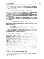
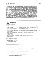
5.1.1 Discontinuous graphs

One very useful application of logical vectors is in plotting discontinuities. The
following script plots the graph, shown in Figure 5.1, defined by
y(x) =

sin (x) ( sin (x) > 0)
0 ( sin (x) ≤ 0)
over the range 0 to 3π:
x=0:pi/20:3*pi;
y = sin(x);
122
Ch05-H8417 5/1/2007 11: 38 page 123
5 Logical vectors
0
0
0.2
0.4
0.6
0.8
1
1.2
1.4
1.6
1.8
2
12345678910
Figure 5.1 A discontinuous graph using logical vectors
y=y.*(y>0);%setnegative values of sin(x) to zero
plot(x, y)
The expression y>0returns a logical vector with 1’s where sin (x) is positive,
and 0’s otherwise. Element-by-element multiplication by y with .* then picks

out the positive elements of y.
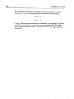
5.1.2 Avoiding division by zero
Suppose you want to plot the graph of sin (x)/x over the range −4π to 4π. The
most convenient way to set up a vector of the x coordinates is
x = -4*pi : pi / 20 : 4*pi;
But then when you try
y = sin(x) ./ x;
you get the Divide by zero warning, because one of the elements of x is
exactly zero. A neat way around this problem is to use a logical vector to replace
123
Ch05-H8417 5/1/2007 11: 38 page 124
Essential MATLAB for Engineers and Scientists
−0.4
−15 −10 −5501015
0.4
0.6
0.8
1
−0.2
0.2
0
Figure 5.2 sin(x)/x
the zero with eps. This MATLAB function returns the difference between 1.0 and
the next largest number which can be represented in MATLAB, i.e. approximately
2.2e-16. Here is how to do it:
x=x+(x==0)*eps;
The expression x==0returns a logical vector with a single 1 for the element
of x which is zero, and so eps is added only to that element. The following script
plots the graph correctly—without a missing segment at x =0 (see Figure 5.2).
x = -4*pi : pi/20 : 4*pi;

x=x+(x==0)*eps; % adjustx=0tox=eps
y = sin(x) ./ x;
plot(x, y)
When x has the value eps, the value of sin(eps)/eps has the correct limiting
value of 1 (check it), instead of NaN (Not-a-Number) resulting from a division
by zero.
124
Ch05-H8417 5/1/2007 11: 38 page 125
5 Logical vectors
1
0.5
−0.5
−5
5
−1
0
0
40
20
−20
−5
5
−40
0
0
(a) (b)
× 10
16
Figure 5.3 Variations on tan(x)
5.1.3 Avoiding infinity

The following script attempts to plot tan (x) over the range −3π/2to3π/2. If
you are not too hot at trig graphs, perhaps you should sketch the graph roughly
with pen and paper before you run the script!
x = -3/2*pi : pi/100 : 3/2*pi;
y = tan(x);
plot(x, y)
The MATLAB plot—Figure 5.3(a)—should look nothing like your sketch. The
problem is that tan (x) approaches ±∞ at odd multiples of π/2. The scale on
the MATLAB plot is therefore very large (about 10
15
), making it impossible to
see the structure of the graph anywhere else.
If you add the statement
y=y.*(abs(y) < 1e10); % remove the big ones
just before the plot statement you’ll get a much nicer graph, as shown in
Figure 5.3(b). The expression abs(y) < 1e10 returns a logical vector which
is zero only at the asymptotes. The graph thus goes through zero at these points,
which incidentally draws nearly vertical asymptotes for you. These ‘asymptotes’
become more vertical as the increment in x becomes smaller.
125
Ch05-H8417 5/1/2007 11: 38 page 126
Essential MATLAB for Engineers and Scientists
5.1.4 Counting random numbers
The function rand returns a (pseudo-)random number in the interval [0, 1);
rand(1, n) returns a row vector of n such numbers.
Try the following exercises on the command line:
1. Set up a vector r with seven random elements (leave out the semicolon so
that you can see its elements):
r = rand(1,7) % no semicolon
Check that the logical expression r < 0.5 gives the correct logical vector.

2. Using the function sum on the logical expression r < 0.5 will effectively
count how many elements of r are less than 0.5. Try it, and check your
answer against the values displayed for r:
sum( r < 0.5 )
3. Now use a similar statement to count how many elements of r are greater
than or equal to 0.5 (the two answers should add up to 7, shouldn’t they?).
4. Since rand generates uniformly distributed random numbers, you would
expect the number of random numbers which are less than 0.5 to get closer
and closer to half the total number as more and more are generated.
Generate a vector of a few thousand random numbers (suppress display
with a semicolon this time) and use a logical vector to count how many are
less than 0.5.
Repeat a few times with a new set of random numbers each time. Because
the numbers are random, you should never get quite the same answer each
time.
Doing this problem without logical vectors is a little more involved. Here is the
program:
tic % start
a = 0; % number >= 0.5
b = 0; % number < 0.5
for n = 1:5000
r = rand; % generate one number per loop
ifr>=0.5
a=a+1;
126
Ch05-H8417 5/1/2007 11: 38 page 127
5 Logical vectors
else
b=b+1;
end;

end;
t = toc; % finish
disp( [’less than 0.5: ’ num2str(a)] )
disp( [’time: ’ num2str(t)] )
It also takes a lot longer. Compare times for the two methods on your computer.
5.1.5 Rolling dice
When a fair dice is rolled, the number uppermost is equally likely to be any inte-
gerfrom1to6.Soifrand is a random number in the range [0, 1), 6 * rand
will be in the range [0, 6), and 6*rand+1will be in the range [1, 7), i.e.
between 1 and 6.9999. Discarding the decimal part of this expression with
floor gives an integer in the required range. Try the following exercises:
1. Generate a vector d of 20 random integers in the range 1 to 6:
d = floor(6 * rand(1, 20)) + 1
2. Count the number of ‘sixes’ thrown by summing the elements of the logical
vector d==6.
3. Verify your result by displaying d.
4. Estimate the probability of throwing a six by dividing the number of sixes
thrown by 20. Using random numbers like this to mimic a real situation
based on chance is called simulation.
5. Repeat with more random numbers in the vector d. The more you have,
the closer the proportion of sixes gets to the theoretical expected value of
0.1667, i.e. 1/6.
6. Can you see why it would be incorrect to use round instead of floor? The
problem is that round rounds in both directions, whereas floor rounds
everything down.
5.2 Logical operators
We saw briefly in Chapter 2 that logical expressions can be constructed not
only from the six relational operators, but also from the three logical operators
127
Ch05-H8417 5/1/2007 11: 38 page 128

Essential MATLAB for Engineers and Scientists
Table 5.1 Logical operators
Operator Meaning
˜ NOT
& AND
| OR
Table 5.2 Truth table (T =true; F =false)
lex1 lex2 ˜ lex1 lex1 & lex2 lex1 & lex2 xor(lex1, lex2)
FFT F F F
FTT F T T
TFF F T T
TTF T T F
shown in Table 5.1. Table 5.2 shows the effects of these operators on the
general logical expressions lex1 and lex2.
The OR operator (|) is technically an inclusive OR, because it is true when either
or both of its operands are true. MATLAB also has an exclusive OR function
xor(a, b) which is 1 (true) only when either but not both of a and b is 1
(Table 5.2).
MATLAB also has a number of functions that perform bitwise logical operations.
See Help on ops.
The precedence levels of the logical operators, among others, are shown in
Table 5.3. As usual, precedences may be overridden with brackets, e.g.
˜0&0
returns 0 (false), whereas
˜(0&0)
returns 1 (true). Some more examples:
(b*b==4*a*c)&(a˜=0)
(final >= 60) & (final < 70)
128
Ch05-H8417 5/1/2007 11: 38 page 129

5 Logical vectors
Table 5.3 Operator precedence (see Help on operator
precedence)
Precedence Operators
1. ()
2. ˆ.ˆ’.’(pure transpose)
3. + (unary plus) - (unary minus) ˜ (NOT)
4. */\ .* ./ .\
5. + (addition) - (subtraction)
6. :
7. ><>=<===˜=
8. & (AND)
9. | (OR)
(a˜=0)|(b˜=0)|(c!=0)
˜((a == 0) & (b == 0) & (c == 0))
It is never wrong to use brackets to make the logic clearer, even if they are
syntactically unnecessary. Incidentally, the last two expressions above are
logically equivalent, and are false only when a =b =c =0. It makes you think,
doesn’t it?
5.2.1 Operator precedence
You may accidentally enter an expression like
2>1&0
(try it) and be surprised because MATLAB (a) accepts it, and (b) returns a value
of 0 (false). It is surprising because:
(a) 2>1&0doesn’t appear to make sense. If you have got this far you
deserve to be let into a secret. MATLAB is based on the notorious language
C, which allows you to mix different types of operators in this way (Pascal,
for example, would never allow such flexibility!).
129
Ch05-H8417 5/1/2007 11: 38 page 130

Essential MATLAB for Engineers and Scientists
(b) We instinctively feel that & should have the higher precedence. 1&0
evaluates to 0, so 2>0should evaluate to 1 instead of 0. The explanation
is due partly to the resolution of surprise (a). MATLAB groups its operators in
a rather curious and non-intuitive way. The complete operator precedence is
given in Table 5.3 (reproduced for ease of reference in Appendix B). (Recall
that the transpose operator ’ performs a complex conjugate transpose on
complex data; the dot-transpose operator .’ performs a ‘pure’ transpose
without taking the complex conjugate.) Brackets always have the highest
precedence.
5.2.2 Danger
I have seen quite a few students incorrectly convert the mathematical inequality
0 < r < 1, say, into the MATLAB expression
0<r<1
Once again, the first time I saw this I was surprised that MATLAB did not report
an error. Again, the answer is that MATLAB doesn’t really mind how you mix up
operators in an expression. It simply churns through the expression according
to its rules (which may not be what you expect).
Suppose r has the value 0.5. Mathematically, the inequality is true for this value
of r since it lies in the required range. However, the expression 0<r<1
is evaluated as 0. This is because the left-hand operation (0 < 0.5)isfirst
evaluated to 1 (true), followed by 1<1which is false.
Inequalities like this should rather be coded as
(0<r)&(r<1)
The brackets are not strictly necessary (see Table 5.3) but they certainly help
to clarify the logic.
5.2.3 Logical operators and vectors
The logical operators can also operate on vectors (of the same size), returning
logical vectors, e.g.
˜(˜[120-40])

replaces all the non-zeros by 1’s, and leaves the 0’s untouched. Try it.
130
Ch05-H8417 5/1/2007 11: 38 page 131
5 Logical vectors
Note that brackets must be used to separate the two ˜’s. Most operators may
not appear directly next to each other (e.g. +˜); if necessary separate them
with brackets.
The script in Section 5.1 that avoids division by zero has the critical statement
x=x+(x==0)*eps;
This is equivalent to
x=x+(˜x)*eps;
Try it, and make sure you understand how it works.
EXERCISE
Work out the results of the following expressions before checking them at the
command line:
a = [-1 0 3];
b=[031];
˜a
a&b
a|b
xor(a, b)
a>0&b>0
a>0|b>0
˜a>0
a+(˜b)
a>˜b
˜a>b
˜(a>b)
5.3 Subscripting with logical vectors
We saw briefly in Chapter 2 that elements of a vector may be referenced with

subscripts, and that the subscripts themselves may be vectors, e.g.
a=[-20159];
a([5 1 3])
returns
9-2 1
131
Ch05-H8417 5/1/2007 11: 38 page 132
Essential MATLAB for Engineers and Scientists
i.e. the fifth, first and third elements of a. In general, if x and v are vectors,
where v has n elements, then x(v) means
[x(v(1)), x(v(2)), , x(v( n))]
Now with a as defined above, see what
a(logical([01010]))
returns. The function logical(v) returns a logical vector, with elements which
are 1 or 0 according as the elements of v are non-zero or 0. (In Version 4 the
logical function was not necessary here—you could use a ‘0-1’ vector directly
as a subscript.)
A summary of the rules for the use of a logical vector as a subscript are as
follows:
➤
A logical vector v may be a subscript of another vector x.
➤
Only the elements of x corresponding to 1’s in v are returned.
➤
x and v must be the same size.
Thus, the statement above returns
05
i.e. the second and fourth elements of a, corresponding to the 1’s in
logical([01010]).
What will

a(logical([11100]))
return? And what about a(logical([00000]))?
Logical vector subscripts provide an elegant way of removing certain elements
from a vector, e.g.
a=a(a>0)
removes all the non-positive elements from a, because a>0returns the
logical vector [00111]. We can verify incidentally that the expression
a>0is a logical vector, because the statement
132
Ch05-H8417 5/1/2007 11: 38 page 133
5 Logical vectors
islogical(a > 0)
returns 1. However, the numeric vector [00111]is not a logical vector;
the statement
islogical([00111])
returns 0.
5.4 Logical functions
MATLAB has a number of useful logical functions that operate on scalars, vec-
tors and matrices. Examples are given in the following list (where x is a vector
unless otherwise stated). See Help on logical functions. (The functions
are defined slightly differently for matrix arguments—see Chapter 6 or Help.)
any(x) returns the scalar 1 (true) if any element of x is non-zero (true).
all(x) returns the scalar 1 if all the elements of x are non-zero.
exist(’a’) returns 1 if a is a workspace variable. For other possible return
values see help. Note that a must be enclosed in apostrophes.
find(x) returns a vector containing the subscripts of the non-zero (true)
elements of x, so for example,
a = a( find(a) )
removes all the zero elements from a! Try it. Another use of find is in
finding the subscripts of the largest (or smallest) elements in a vector,

when there is more than one. Enter the following:
x=[81-486];
find(x >= max(x))
This returns the vector [1 4], which are the subscripts of the largest
element (8). It works because the logical expression x >= max(x) returns
a logical vector with 1’s only at the positions of the largest elements.
isempty(x) returns 1 if x is an empty array and 0 otherwise. An empty array
has a size of 0-by-0.
133
Ch05-H8417 5/1/2007 11: 38 page 134
Essential MATLAB for Engineers and Scientists
isinf(x) returns 1’s for the elements of x which are +Inf or −Inf, and 0’s
otherwise.
isnan(x) returns 1’s where the elements of x are NaN and 0’s otherwise. This
function may be used to remove NaNs from a set of data. This situation
could arise while you are collecting statistics; missing or unavailable values
can be temporarily represented by NaNs. However, if you do any calculations
involving the NaNs, they propagate through intermediate calculations to the
final result. To avoid this, the NaNs in a vector may be removed with a
statement like
x(isnan(x))=[]
MATLAB has a number of other logical functions starting with the characters
is. See is* in the Help index for the complete list.
5.4.1 Using any and all
Because any and all with vector arguments return scalars, they are particularly
useful in if statements. For example,
if all(a >= 1)
do something
end
means ‘if all the elements of the vector a are greater than or equal to 1, then

do something’.
Recall from Chapter 2 that a vector condition in an if statement is true only if
all its elements are non-zero. So if you want to execute statement below when
two vectors a and b are equal (i.e. the same) you could say
ifa==b
statement
end
since if considers the logical vector returned by a==btrue only if every
element is a 1.
If, on the other hand, you want to execute statement specifically when the
vectors a and b are not equal, the temptation is to say
134
Ch05-H8417 5/1/2007 11: 38 page 135
5 Logical vectors
if a ˜= b % wrong wrong wrong!!!
statement
end
However this will not work, since statement will only execute if each of the
corresponding elements of a and b differ. This is where any comes in:
if any(a ˜= b) % right right right!!!
statement
end
This does what is required since any(a ˜= b) returns the scalar 1 if any
element of a differs from the corresponding element of b.
5.5 Logical vectors instead of elseif ladders
Those of us who grew up on more conventional programming languages in the
last century may find it difficult to think in terms of using logical vectors when
solving general problems. It’s a nice challenge whenever writing a program to
ask yourself whether you can possibly use logical vectors. They are almost
always faster than other methods, although often not as clear to read later.

You must decide when it’s important for you to use logical vectors. But it’s a
very good programming exercise to force yourself to use them whenever pos-
sible! The following example illustrates these points by first solving a problem
conventionally, and then with logical vectors.
It has been said that there are two unpleasant and unavoidable facts of life:
death and income tax. A very simplified version of how income tax is calculated
could be based on the following table:
Taxable income Tax payable
$10 000 or less 10 percent of taxable income
between $10 000 and $1000 +20 percent of amount by which
$20 000 taxable income exceeds $10 000
more than $20 000 $3000 +50 percent of amount by which
taxable income exceeds $20 000
The tax payable on a taxable income of $30 000, for example, is
$3000 + 50 percent of ($30 000 −$20 000), i.e. $8000.
135
Ch05-H8417 5/1/2007 11: 38 page 136
Essential MATLAB for Engineers and Scientists
We would like to calculate the income tax on the following taxable incomes (in
dollars): 5000, 10 000, 15 000, 30 000 and 50000.
The conventional way to program this problem is to set up a vector with the
taxable incomes as elements and to use a loop with an elseif ladder to
process each element, as follows:
% Income tax the old-fashioned way
inc = [5000 10000 15000 30000 50000];
for ti = inc
if ti < 10000
tax = 0.1 * ti;
elseif ti < 20000
tax = 1000 + 0.2 * (ti - 10000);

else
tax = 3000 + 0.5 * (ti - 20000);
end;
disp( [ti tax] )
end;
Here is the output, suitably edited (note that the amount of tax paid changes
continuously between tax ‘brackets’—each category of tax is called a bracket):
Taxable income Income tax
5000.00 500.00
10000.00 1000.00
15000.00 2000.00
30000.00 8000.00
50000.00 18000.00
Now here is the logical way:
% Income tax the logical way
inc = [5000 10000 15000 30000 50000];
tax = 0.1 * inc .* (inc <= 10000);
tax = tax + (inc > 10000 & inc <= 20000)
136
Ch05-H8417 5/1/2007 11: 38 page 137
5 Logical vectors
.* (0.2 * (inc-10000) + 1000);
tax = tax + (inc > 20000) .* (0.5 * (inc-20000) + 3000);
disp( [inc’ tax’] );
To understand how it works, it may help to enter the statements on the
command line. Start by entering the vector inc as given. Now enter
inc <= 10000
which should give the logical vector [11000]. Next enter
inc .* (inc <= 10000)
which should give the vector [5000 10000000]. This has success-

fully selected only the incomes in the first bracket. The tax for these incomes
is then calculated with
tax = 0.1 * inc .* (inc <= 10000)
which returns [500 1000000].
Now for the second tax bracket. Enter the expression
inc > 10000 & inc <= 20000
which returns the logical vector [00100], since there is only one
income in this bracket. Now enter
0.2 * (inc-10000) + 1000
This returns [0 1000 2000 5000 9000]. Only the third entry is cor-
rect. Multiplying this vector by the logical vector just obtained blots out the other
entries, giving [00200000]. The result can be safely added to the
vector tax since it will not affect the first two entries already there.
I am sure you will agree that the logical vector solution is more interesting than
the conventional one!
137