Essential MATLAB for Engineers and Scientists PHẦN 8 pptx

Ch12-H8417 5/1/2007 11: 41 page 289
12 More graphics
z = peaks(25);
c(:,:,1) = rand(25);
c(:,:,2) = rand(25);
c(:,:,3) = rand(25);
surf(z,c,’facecolor’,’interp’,’facelighting’,’phong’,
’edgecolor’,’none’)
camlight right
The possibilities for the facelighting property of the surface object are
none, flat (uniform color across each facet), gouraud or phong. The last
two are the names of lighting algorithms. Phong lighting generally produces
better results, but takes longer to render than Gouraud lighting. Remember
that you can see all a surface object’s properties by creating the object with a
handle and using get on the object’s handle.
This one’s quite stunning:
[xy]=meshgrid(-8 : 0.5 : 8);
r = sqrt(x.ˆ2 + y.ˆ2) + eps;
z = sin(r) ./ r;
surf(x,y,z,’facecolor’,’interp’,’edgecolor’,’none’,
’facelighting’,’phong’)
colormap jet
daspect([5 5 1])
axis tight
view(-50, 30)
camlight left
For more information on lighting and the camera see the sections Lighting as a
Visualization Tool and Defining the View in Using MATLAB: 3-D Visualization.
12.6 Saving, printing and exporting graphs
12.6.1 Saving and opening figure files
You can save a figure generated during a MATLAB session so that you can open

it in a subsequent session. Such a file has the .fig extension.
➤
Select Save from the figure window File menu.
➤
Make sure the Save as type is .fig.
To open a figure file select Open from the File menu.
289
Ch12-H8417 5/1/2007 11: 41 page 290
Essential MATLAB for Engineers and Scientists
12.6.2 Printing a graph
You can print everything inside a figure window frame, including axis labels and
annotations:
➤
To print a figure select Print from the figure window File menu.
➤
If you have a black and white printer, colored lines and text are ‘dithered
to gray’ which may not print very clearly in some cases. In that case select
Page Setup from the figure File menu. Select the Lines and Text tab and
click on the Black and white option for Convert solid colored lines to:.
12.6.3 Exporting a graph
A figure may be exported in one of a number of graphics formats if you want to
import it into another application, such as a text processor. You can also export
it to the Windows clipboard and paste it from there into an application.
To export to the clipboard:
➤
Select Copy Figure from the figure window’s Edit menu (this action copies
to the clipboard).
➤
Before you copy to the clipboard you may need to adjust the figure’s set-
tings. You can do this by selecting Preferences from the figure’s File menu.

This action opens the Preferences panel, from which you can select Figure
Copy Template Preferences and Copy Options Preferences to adjust the
figure’s settings.
You may also have to adjust further settings with Page Setup from the
figure’s File menu.
To export a figure to a file in a specific graphics format:
➤
Select Export from the figure’s File menu. This action invokes the Export
dialogue box.
➤
Select a graphics format from the Save as type list, e.g. EMF (enhanced
metafiles), JPEG, etc. You may need to experiment to find the best format
for the target application you have in mind.
For example, to insert a figure into a Word document, I find it much easier
first to save it in EMF or JPEG format and then to insert the graphics file
into the Word document, rather than to go the clipboard route (there are
more settings to adjust that way).
290
Ch12-H8417 5/1/2007 11: 41 page 291
12 More graphics
For further details consult the section Basic Printing and Exporting in Using
MATLAB: Graphics.
Summary
➤
MATLAB graphics objects are arranged in a parent–child hierarchy.
➤
A handle may be attached to a graphics object at creation; the handle may be used
to manipulate the graphics object.
➤
If h is the handle of a graphics object, get(h) returns all the current values of the

object’s properties. set(h) shows you all the possible values of the properties.
➤
The functions gcf, gca and gco return the handles of various graphics objects.
➤
Use set to change the properties of a graphics object.
➤
A graph may be edited to a limited extent in plot edit mode, selected from the figure
window (Tools -> Edit Plot). More general editing can be done with the Property
Editor (Edit -> Figure Properties from the figure window).
➤
The most versatile way to create animations is by using the Handle Graphics
facilities. Other techniques involve comet plots and movies.
➤
Indexed coloring may be done with colormaps.
➤
Graphs saved to .fig files may be opened in subsequent MATLAB sessions.
➤
Graphs may be exported to the Windows clipboard, or to files in a variety of graphics
formats.
291
Ch13-H8417 5/1/2007 11: 41 page 292
13
*Graphical User
Interfaces (GUIs)
The objectives of this chapter are to introduce you to the basic concepts involved
in writing your own graphical user interfaces, including:
➤ Figure files.
➤ Application M-files.
➤ Callback functions.
The script files we have written so far in this book have had no interaction

with the user, except by means of the occasional input statement. Modern
users, however, have grown accustomed to more sophisticated interaction with
programs, by means of windows containing menus, buttons, drop-down lists,
etc. This way of interacting with a program is called a graphical user interface,
or GUI for short (pronounced ‘gooey’), as opposed to a text user interface by
means of command-line based input statements.
The MATLAB online documentation has a detailed description of how to write
GUIs in MATLAB, to be found in Using MATLAB: Creating Graphical User Inter-
faces. This chapter presents a few examples illustrating the basic concepts.
Hahn, the original author (of the first two editions of this book) stated that he
“spent a day or two reading MATLAB’s documentation in order to write the GUIs
in this chapter.” He pointed out that he seldom had such fun programming!
13.1 Basic structure of a GUI
➤ MATLAB has a facility called GUIDE (Graphical User Interface Development
Environment) for creating and implementing GUIs. You start it from the
command line with the command guide.
Ch13-H8417 5/1/2007 11: 41 page 293
13 Graphical User Interfaces (GUIs)
➤ The guide command opens an untitled figure which contains all the GUI
tools needed to create and lay out the GUI components (e.g. pushbuttons,
menus, radio buttons, popup menus, axes, etc.). These components are
called uicontrols in MATLAB (for user interface controls).
➤ GUIDE generates two files that save and launch the GUI: a FIG-file and an
application M-file.
➤ The FIG-file contains a complete description of the GUI figure, i.e. whatever
uicontrols and axes are needed for your graphical interface.
➤ The application M-file (the file you run to launch the GUI) contains the
functions required to launch and control the GUI. The application M-file does
not contain the code that lays out the GUI components; this information is
saved in the FIG-file.

The GUI is controlled largely by means of callback functions, which are
subfunctions in the application M-file.
➤ Callback functions are written by you and determine what action is taken
when you interact with a GUI component, e.g. click a button. GUIDE gen-
erates a callback function prototype for each GUI component you create.
You then use the Editor to fill in the details.
13.2 A first example: getting the time
For our first example we will create a GUI with a single pushbutton. When you
click the button the current time should appear on the button (Figure 13.1). Go
through the following steps:
➤ Run guide from the command line. This action opens the Layout Editor
(Figure 13.2).
➤ We want to place a pushbutton in the layout area. Select the pushbutton
icon in the component palette to the left of the layout area. The cursor
changes to a cross. You can use the cross either to select the position of
the top-left corner of the button (in which it has the default size), or you
can set the size of the button by clicking and dragging the cursor to the
bottom-right corner of the button.
A button imaginatively names Push Button appears in the layout area.
➤ Select the pushbutton (click on it). Right-click for its context menu and
select Inspect Properties. Use the Property Inspector to change the but-
ton’s String property to Time. The text on the button in the layout area
will change to Time.
293
Ch13-H8417 5/1/2007 11: 41 page 294
Essential MATLAB for Engineers and Scientists
Figure 13.1 Click the button to see the time
Figure 13.2 GUIDE Layout Editor
294
Ch13-H8417 5/1/2007 11: 41 page 295

13 Graphical User Interfaces (GUIs)
Note that the Tag property of the button is set to pushbutton1. This is the
name GUIDE will use for the button’s callback function when it generates
the application M-file in a few minutes. If you want to use a more meaningful
name when creating a GUI which may have many such buttons, now is the
time to change the tag.
If you change a component’s tag after generating the application M-file you
have to change its callback function name by hand (and all references to
the callback). You also have to change the name of the callback function
in the component’s Callback property. For example, suppose you have
generated an application M-file with the name myapp.m, with a pushbutton
having the tag pushbutton1. The pushbutton’s Callback property will
be something like
myapp(’mybutton_Callback’,gcbo,[],guidata(gcbo))
If you want to change the tag of the pushbutton to Open, say, you will need
to change its Callback property to
myapp(’Open_Callback’,gcbo,[],guidata(gcbo))
➤ Back in the Layout Editor select your button again and right-click for the
context menu. Select Edit Callback.
A dialog box appears for you to save your FIG-file. Choose a directory and
give a filename of time.fig—make sure that the .fig extension is used.
GUIDE now generates the application M-file (time.m), which the Editor
opens for you at the place where you now have to insert the code for
whatever action you want when the Time button is clicked:
function varargout = pushbutton1_Callback(h,
eventdata, handles, varargin)
% Stub for Callback of the uicontrol handles.
pushbutton1.
disp(’pushbutton1 Callback not implemented yet.’)
Note that the callback’s name is pushbutton1_Callback where

pushbutton1 is the button’s Tag property.
Note also that the statement
disp(’pushbutton1 Callback not implemented yet.’)
is automatically generated for you.
➤ If you are impatient to see what your GUI looks like at this stage click the
Activate Figure button at the right-hand end of the Layout Editor toolbar.
295
Ch13-H8417 5/1/2007 11: 41 page 296
Essential MATLAB for Engineers and Scientists
An untitled window should appear with a Time button in it. Click the Time
button—the message
pushbutton1 Callback not implemented yet
should appear in the Command Window.
➤ Now go back to the (M-file) Editor to change the pushbutton1_Call back
function. Insert the following lines of code, which are explained below:
% get time
d = clock;
% convert time to string
time = sprintf(’%02.0f:%02.0f:%02.0f’,d(4),d(5),
d(6));
% change the String property of pushbutton1
set(gcbo,’String’,time)
The function clock returns the date and time as a six-component vector
in the format
[year month day hour minute seconds]
The sprintf statement converts the time into a string time in the usual
format, e.g. 15:05:59
➤ The last statement is the most important one as it is the basis of the
button’s action:
set(gcbo,’String’,time)

It is the button’s String property which is displayed on the button in the
GUI. It is therefore this property which we want to change to the current
time when it is clicked.
The command gcbo stands for ‘get callback object’, and returns the handle
of the current callback object, i.e. the most recently activated uicontrol. In
this case the current callback object is the button itself (it could have
been some other GUI component). The set statement then changes the
String property of the callback object to the string time which we have
created.
Easy!
➤ Save the application M-file and return to the Layout Editor. For complete-
ness give the entire figure a name. Do this by right-clicking anywhere in the
layout area outside the Time button. The context menu appears. Select
Property Inspector. This time the Property Inspector is looking at the
296
Ch13-H8417 5/1/2007 11: 41 page 297
13 Graphical User Interfaces (GUIs)
figure’s properties (instead of the pushbutton’s properties) as indicated
at the top of its window. Change the Name property to something suitable
(like Time).
➤ Finally, click Activate Figure again in the Layout Editor. Your GUI should now
appear in a window entitled Time. When you click the button the current
time should appear on the button.
➤ If you want to run your GUI from the command line, enter the application
M-file name.
13.2.1 Exercise
You may have noticed that graphics objects have a Visible property. See if you
can write a GUI with a single button which disappears when you click on it! This
exercise reminds me of a project my engineering friends had when I was a first-
year student. They had to design a black box with a switch on the outside. When

it was switched on a lid opened, and a hand came out of the box to switch if off …
13.3 Newton again
Our next example is a GUI version of Newton’s method to find a square root:
you enter the number to be square-rooted, press the Start button, and some
iterations appear on the GUI (Figure 13.3).
Figure 13.3 Square roots with Newton’s method.
297
Ch13-H8417 5/1/2007 11: 41 page 298
Essential MATLAB for Engineers and Scientists
We will use the following uicontrols from the component palette in the Layout
Editor:
➤
a static text control to display the instruction Enter number to square
root and press Start: (static text is not interactive, so no callback
function is generated for it);
➤
an edit text control for the user to enter the number to be square-rooted;
➤
a pushbutton to start Newton’s method;
➤
a static text control for the output, which will consist of several iterations.
You can of course send the output to the command line with disp.
➤
We will also make the GUI window resizable (did you notice that you couldn’t
resize the Time window in the previous example?).
Proceed as follows:
➤
Run guide from the command line. When the Layout Editor starts right-
click anywhere in the layout area to get the figure’s Property Inspector and
set the figure’s Name property to Newton.

➤
Now let’s first make the GUI resizable. Select Tools in the Layout Editor’s
toolbar and then Application Options. There are three Resize behav-
ior options: Non-resizable (the default), Proportional and User-specified.
Select Proportional. Note that under Proportional when you resize the win-
dow the GUI components are also resized, although the font size of labels
does not resize.
➤
Place a static text control for the instruction to the user in the layout area.
Note that you can use the Alignment Tool in the Layout Editor toolbar to
align controls accurately if you wish. You can also use the Snap to Grid
option in the Layout menu. If Snap to Grid is checked then any object
which is moved to within nine pixels of a grid line jumps to that line.
You can change the grid spacing with Layout -> Grid and Rulers -> Grid
size.
Use the Property Inspector to change the static text control’s String
property to Enter number to square root and press Start:
➤
Place an edit text control on the layout area for the user to input the number
to be square-rooted. Set its String property to blank. Note that you don’t
need to activate the Property Inspector for each control. Once the Property
Inspector has been started it switches to whichever object you select in
the layout area. The tag of this component will be edit1 since no other
edit text components have been created.
298
Ch13-H8417 5/1/2007 11: 41 page 299
13 Graphical User Interfaces (GUIs)
➤ Activate the figure at this stage (use the Activate Figure button in the Layout
Editor toolbar), and save it under the name Newton.fig. The application
M-file should open in the Editor. Go to the edit1_Callback subfunction

and remove the statement
disp(’edit1 Callback not implemented yet.’)
No further coding is required in this subfunction since action is to be
initiated by the Start button.
Remember to remove this disp statement from each callback subfunction
as you work through the code.
➤
Insert another static text control in the layout area for the output of New-
ton’s method. Make it long enough for five or six iterations. Set its String
property to Output and its HorizontalAlignment to left (so that
output will be left-justified).
Make a note of its tag, which should be text2 (text1 being the tag of
the other static text control).
➤
Place a pushbutton in the layout area. Set its String property to Start.
Its tag should be pushbutton1.
➤
Activate the figure again so that the application M-file gets updated. We
now have to program the pushbutton1_Callback subfunction to
– get the number to be square-rooted from the edit text control;
– run Newton’s method to estimate the square root of this number;
– put the output of several iterations of Newton’s method in the Output
static text control;
– clear the edit text control in readiness for the next number to be entered
by the user.
These actions are achieved by the following code, which is explained below:
function varargout = pushbutton1_Callback(h,
eventdata, handles, varargin)
% Stub for Callback of the uicontrol handles.
pushbutton1.

a = str2num(get(handles.edit1,’String’));
x = a; % initial guess
for i = 1:8
x = (x + a/x)/2;
str(i) = sprintf(’%g’,x);
end
299
Ch13-H8417 5/1/2007 11: 41 page 300
Essential MATLAB for Engineers and Scientists
set(handles.edit1,’String’,’’);
set(handles.text2,’String’,str);
If you have read the helpful comments generated in the application M-file
you will have seen that the input argument handles is a structure con-
taining handles of components in the GUI, using their tags as fieldnames.
This mechanism enables the various components to communicate with
each other in the callback subfunctions. This is why it is not a good idea
to change a tag after its callback subfunction has been generated; you
would then need to change the name of the callback function as well as
any references to its handle.
When you type anything into an edit text control, its String property is
automatically set to whatever you type. The first statement
a = str2num(get(handles.edit1,’String’));
uses the handle of the edit text control to get its String property (assum-
ing it to have been correctly entered—note that we are not trying to catch
any user errors here). The str2num function converts this string to the
number a.
A for loop then goes through eight iterations of Newton’s method to
estimate the square root of a.
The variable x in the loop contains the current estimate. sprintf converts
the value of x to a string using the g (general) format code. The resulting

string is stored in the ith element of a cell array str. Note the use of curly
braces to construct the cell array. This use of a cell array is the easiest
way to put multiple lines of text into an array for sending to the text2
static text.
The statement
set(handles.edit1,’String’,’’);
clears the display in the edit text control.
Finally, the statement
set(handles.text2,’String’,str);
sets the String property of the text2 static text control to the cell array
containing the output.
➤
Save your work and activate the figure again to test it.
300
Ch13-H8417 5/1/2007 11: 41 page 301
13 Graphical User Interfaces (GUIs)
13.4 Axes on a GUI
This example demonstrates how to plot graphs in axes on a GUI. We want a
button to draw the graph, one to toggle the grid on and off, and one to clear the
axes (Figure 13.4). The only new feature in this example is how to plot in axes
which are part of the GUI. We address this issue first.
➤
Open a new figure in the GUIDE Layout Editor. Right-click anywhere in the
layout area to open the figure’s Property Inspector. Note that the figure
has a HandleVisibility property which is set to off by default. This
prevents any drawing in the figure. For example, you would probably not
want plot statements issued at the command-line to be drawn on the GUI.
However, you can’t at the moment draw on the GUI from within the GUI
either! The answer is to set the figure’s HandleVisibility property to
callback. This allows any GUI component to plot graphs on axes which

are part of the GUI, while still protecting the GUI from being drawn all over
from the command line.
Figure 13.4 Axes on a GUI.
301
Ch13-H8417 5/1/2007 11: 41 page 302
Essential MATLAB for Engineers and Scientists
➤
Place an axes component on the GUI. Its HandleVisibility should
be on.
➤
Place a pushbutton (tag pushbutton1) on the GUI and change its String
property to Plot. Save the figure (if you have not already) under the
name Plotter and generate the application M-file. Edit the pushbutton’s
callback subfunction to draw any graph, e.g. sin(x).
➤
Place pushbutton2 on the GUI to toggle the grid and put the command
grid in its callback subfunction.
➤
Put pushbutton3 on the GUI with the command cla to clear the axes.
➤
Save and reactivate the figure. Test it out. Change the figure’s
HandleVisibility back to off, activate the figure, and see what
happens.
Note that the figure object has a IntegerHandle property set to off.
This means that even if HandleVisibility is on you can’t plot on the
axes from the command line (or another GUI) because a figure needs an
integer handle in order to be accessed. If you want to be able to draw all
over your GUI from the command line just set the figure’s IntegerHandle
to on.
13.5 Adding color to a button

The final example in this chapter shows you how to add an image to a button.
➤
Create a GUI with a single pushbutton in it.
➤
Set the button’s Units property to pixels.
➤
Expand the button’s Position property and set width to 100 and
height to 50.
➤
Insert the following code in the button’s callback subfunction:
a(:,:,1) = rand*ones(50,100);
a(:,:,2) = rand*ones(50,100);
a(:,:,3) = rand*ones(50,100);
set(h,’CData’,a);
➤
The matrix a defines a truecolor image the same size as the pushbutton,
with each pixel in the image the same (random) color.
The third dimension of a sets the RGB video intensities. If, for example,
you would prefer the button to be a random shade of green, say, try
302
Ch13-H8417 5/1/2007 11: 41 page 303
13 Graphical User Interfaces (GUIs)
a(:,:,1) = zeros(50,100);
a(:,:,2) = rand*ones(50,100);
a(:,:,3) = zeros(50,100);
➤
The input argument h of the callback subfunction is the callback object’s
handle (obtained from gcbo).
➤
An image may also be added to a toggle button control.

Summary
➤
GUIs are designed and implemented by MATLAB’s GUIDE facility.
➤
The guide command starts the Layout Editor, which is used to design GUIs.
➤
GUIDE generates a FIG-file, which contains the GUI design, and an application M-file,
which contains the code necessary to launch and control the GUI.
➤
You launch the GUI by running its application M-file.
➤
Many GUI components have callback subfunctions in the application M-file where you
write the code to specify the components’ actions.
➤
You use the Property Inspector to set a GUI component’s properties at the design
stage.
➤
The handles of all GUI components are fields in the handles structure in the
application M-file. These handles are available to all callback subfunctions and
enable you to find and change components’ properties.
303
This page intentionally left blank
Ch14-H8417 5/1/2007 11: 42 page 305
Part II
Applications
Part II is on applications. Since this is an introductory course, the applications
are not extensive. They are illustrative. You ought to recognize that the kinds of
problems you actually can solve with MATLAB are much more challenging than
the examples provided. More is said on this matter at the beginning of Chapter
14. The goal of this part is to scratch the surface of the true power of tools like

MATLAB and to show how you can use it in a variety of ways.
This page intentionally left blank
Ch14-H8417 5/1/2007 11: 42 page 307
14
Dynamical systems
The objective of this chapter is to discuss the importance of learning to use tools
like MATLAB. MATLAB and companion toolboxes provide engineers, scientists,
mathematicians, and students of these fields with an environment for technical
computing applications. It is much more than a programming language like C,
C++ or Fortran. Technical computing includes mathematical computation, anal-
ysis, visualization, and algorithm development. The MathWork website describes
‘The Power of Technical Computing with MATLAB’ as follows:
➤ Whatever the objective of your work—an algorithm, an analysis, a graph,
a report, or a software simulation—technical computing with MATLAB
lets you work more effectively and efficiently. The flexible MATLAB envi-
ronment lets you perform advanced analyses, visualize data, and develop
algorithms by applying the wealth of functionality available. With its more
than 1000 mathematical, statistical, scientific and engineering functions,
MATLAB gives you immediate access to high-performance numerical com-
puting. This functionality is extended with interactive graphical capabilities
for creating plots, images, surfaces, and volumetric representations.
➤ The advanced toolbox algorithms enhance MATLAB’s functionality in
domains such as signal and image processing, data analysis and statis-
tics, mathematical modeling, and control design. Toolboxes are col-
lections of algorithms, written by experts in their fields, that provide
application-specific numerical, analysis, and graphical capabilities. By
relying on the work of these experts, you can compare and apply a number
of techniques without writing code. As with MATLAB algorithms, you can
customize and optimize toolbox functions for your project requirements.
In this chapter we are going to examine the application of MATLAB capabili-

ties to four relatively simple problems in engineering science. The problems
are the deflection of a cantilever beam subject to a uniform load, a single-loop
closed electrical circuit, the free fall problem, and an extension of the projectile
problem discussed in Chapter 3. The first problem is on a structural element
you will investigate in your first course in engineering mechanics. The structural
Ch14-H8417 5/1/2007 11: 42 page 308
Essential MATLAB for Engineers and Scientists
element is the cantilever beam, which is one of the primary elements of engi-
neered structures, e.g. buildings and bridges. We examine the deflection of this
beam with a constant cross-section when subject to a uniform distribution of
load, e.g. its own weight.
The second problem is an examination of the equation that describes the ‘flow’
of electrical current in a simple closed-loop electrical circuit. You examine this
type of problem in your first course in electrical science.
The third problem is the free fall of an object in a gravitational field with constant
acceleration, g. This is one of the first problems you examine in your first
course in physics. We examine the effect of friction on the free-fall problem
and, hence, learn that with friction (i.e. air resistance) the object can reach a
terminal velocity.
The fourth problem is an extension of the projectile that takes into account air
resistance (you learn about air resistance in your first course in fluid mechanics).
By an examination of this problem, you will learn why golfers do not hit the ball
from the tee at 45 degrees from the horizontal (which is the optimum angle for
the furthest distance of travel of a projectile launched in frictionless air).
Before we begin, you must keep in mind that this is not a book on engineering or
science; it is an introduction to the essential elements of MATLAB, a powerful
technical analysis tool. In this and subsequent chapters you will scratch the
surface of its power by solving some relatively simple problems that you have
encountered or will encounter early in your science or engineering education.
Keep in mind that MATLAB is a tool that can be used for a number of very

productive purposes. One purpose is to learn how to write programs to inves-
tigate topics you confront in the classroom. You can extend your knowledge of
MATLAB by self-learning to apply the utilities and any of the toolboxes that are
available to you to solve technical problems. This tool requires a commitment
from you to continue to discover and to use the power of the tool as part of
your continuing education. Developing high-quality computer programs within
the MATLAB environment in order to solve technical problems requires that you
use the utilities available. If you need to write your own code you should, if
at all possible, include the utilization of generic solvers of particular types of
equations that are available in MATLAB. Of course, to do this you need to learn
more advanced mathematics, science and engineering. You will certainly have
the opportunity to do this after freshman year.
As a student majoring in science and engineering you will take at least five
semesters of mathematics. The fifth course is usually titled Advanced Calculus,
Advanced Engineering Mathematics, Applied Mathematics, or Methods of Math-
ematical Physics. Topics covered in this course are typically ordinary differential
308
Ch14-H8417 5/1/2007 11: 42 page 309
14 Dynamical systems
equations, systems of differential equations (including nonlinear systems),
linear algebra (including matrix and vector algebra), vector calculus, Fourier
analysis, Laplace transforms, partial differential equations, complex analysis,
numerical methods, optimization, probability and statistics. By clicking the
question mark (?) near the center of the uppermost toolbar in the MATLAB
desktop, as you already know, opens the help browser. Scan the topics and
find utilitites and examples of approaches to solve problems in all of these
subjects and more.
The Control Systems Toolbox is an example of one of the numerous engineering
and scientific toolboxes that have been developed to advance the art of doing
science and engineering. SIMULINK and Symbolics are also very important tool-

boxes. The latter two are included with your ‘student version’ of MATLAB. One
of the big advantages of SIMULINK, in addition to being a graphical algorithm-
development and programming environment, is that it is useful when using the
computer to measure, record and access data from laboratory experiments
or data from industrial-process monitoring systems. Symbolics is very useful
because it allows you to do symbolic mathematics, e.g. integrating functions
like the ones you integrate in your study of the calculus. All of the mathematical
subjects investigated by you, as a science or engineering major, are applied
in your science and engineering courses. They are the same techniques that
you will apply as a professional (directly or indirectly depending on the software
tools available within the organization that you are employed). Thus, you can use
your own copy of MATLAB to help you understand the mathematical and software
tools that you are expected to apply in the classroom as well as on the job.
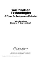
14.1 Cantilever beam
In this section we want to examine the problem of the cantilever beam. The
beam and its deflection under load is illustrated in Figure 14.1 below, which is
generated by the script m-file created to solve the problem posed next. Many
structural mechanics formulae are available in Formulas for Stress and Strain,
Fifth Edition by Raymond J. Roark and Warren C. Young, published by McGraw-
Hill Book Company (1982). For a uniformly loaded span of a cantilever beam
attached to a wall at x =0 with the free end at x =L, the formula for the vertical
displacement from y =0 under the loaded condition with y the coordinate in the
direction opposite that of the load can be written as follows:
Y =
y 24EI
wL
4
=−

X

4
−4 X
3
+6 X
2

,
309
Ch14-H8417 5/1/2007 11: 42 page 310
Essential MATLAB for Engineers and Scientists
0 0.5 1 1.5
Ϫ4
Ϫ3.5
Ϫ3
Ϫ2.5
Ϫ2
Ϫ1.5
Ϫ1
Ϫ0.5
0
0.5
1
X
Y
Unloaded cantilever beam
Uniformly loaded beam
Figure 14.1 Deflection of a cantilever beam. The vertical deflection of a uniformly loaded
cantilever beam
where X =x/L, E is a material property known as the modulus of elasticity, I is
a geometric property of the cross-section of the beam known as the moment

of inertia, L is the length of the beam extending from the wall from which
it is mounted, and w is the load per unit width of the beam (this is a two-
dimensional analysis). The formula was put into dimensionless form to answer
the following question: What is the shape of the deflection curve when the beam
is in its loaded condition and how does it compare with its unloaded perfectly
horizontal orientation? The answer will be provided graphically. This is easily
solved by using the following script:
%
% The deflection of a cantilever beam under a uniform
%load
% Script by D.T.V. September 2006
%
% Step 1: Select the distribution of X’s from 0 to 1
% where the deflections to be plotted are to be
%determined.
%
X = 0:.01:1;
%
310
Ch14-H8417 5/1/2007 11: 42 page 311
14 Dynamical systems
% Step 2: Compute the deflections Y at eaxh X. Note that
% YE is the unloaded position of all points on the beam.
%
Y=-(X.ˆ4-4*X.ˆ3+6*X.ˆ2 );
YE=0;
%
% Step 3: Plot the results to illustrate the shape of the
% deflected beam.
%

plot([0 1],[0 0],’ ’,X,Y,’LineWidth’,2)
axis([0,1.5,-4, 1]),title(’Deflection of a cantilever
beam’)
xlabel(’X’),ylabel(’Y’)
legend(’Unloaded cantilever beam’,’Uniformly loaded
beam’)
%
% Step 4: Stop
Again, the results are plotted in Figure 14.1. It looks like the beam is deflected
tremendously. The actual deflection will not necessarily be so dramatic once the
actual material properties are substituted to determine y and x in, say, meters.
The scaling, i.e. rewriting the equation in dimensionless form in terms of the
unitless quantities Y and X, provides insight into the shape of the curve. In
addition, the shape is independent of the material as long as it is a material
with uniform properties and the geometry has a uniform cross-sectional area,
e.g. a rectangular area of height h and width b that is independent of the
distance along the span (or length) L.
14.2 Electric current
When you investigate electrical science you investigate circuits with a variety of
components. In this section we will solve the governing equation to examine the
dynamics of a single closed-loop electrical circuit. The loop contains a voltage
source, V (e.g. a battery), a resistor, R (i.e. an energy dissipation device), an
inductor, L (i.e. an energy storage device), and a switch which is instantaneously
closed at time t =0. From Kirchhoff’s law, as described in the book by Ralph J.
Smith entitled Circuits, Devices, and Systems, published by John Wiley & Sons,
Inc. (1967), the equation describing the response of this system from an initial
state of zero current is as follows:
L
di
dt

+Ri = V,
where i is the current. At t =0 the switch is engaged to close the circuit and
initiate the current. At this instant of time the voltage is applied to the resistor
311
Ch14-H8417 5/1/2007 11: 42 page 312
Essential MATLAB for Engineers and Scientists
and inductor (which are connected in series) instantaneously. The equation
describes the value of i as a function of time after the switch is engaged.
Hence, for the present purpose, we want to solve this equation to determine i
versus t graphically. Rearranging this equation, we get
di
dt
+
R
L
i =
V
L
.
The solution, by inspection (another method that you learn when you take
differential equations), is
i =
V
R

1 − e
−
R
L
t


.
This solution is checked with the following script:
%
% Script to check the solution to the soverning
% equation for a simple circuit, i.e. to check
% that
% i = (V/R) * (1 - exp(-R*t/L))
%
% is the solution to the following ODE
%
% di/dt + (R/L)*i-V/L=0
%
% Step 1: We will use the Symbolics tools; hence,
% define the symbols as follows
%
symsiVRLt
%
% Step 2: Construct the solution for i
%
i = (V/R)*(1-exp(-R*t/L) );
%
% Step 3: Find the derivative of i
%
didt = diff(i,t);
%
% Step 4: Sum the terms in ODE
%
didt + (R/L)*i-V/L;
%

% Step 5: Is the answer ZERO?
%
simple(ans)
%
% Step 6: What is i att=0?
312
Ch14-H8417 5/1/2007 11: 42 page 313
14 Dynamical systems
%
subs(i,t,0)
%
% REMARK: Both answers are zero; hence,
% the solution is correct and the
% initial condition is correct.
%
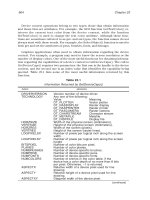
% Step 7: To illustrate the behavior of the
% current, plot i vs. t for V/R = 1
% and R/L = 1. The curve illustrates
% the fact that the current approaches
% i = V/R exponentially.
%
V=1;R=1;L=1;
t=0:0.01 : 6;
i = (V/R)*(1-exp(-R.*t/L) );
plot(t,i,’ro’), title(Circuit problem example)
xlabel(’time, t’),ylabel(’current, i’)
%
0 1 2 3 4 5 6
0
0.1

0.2
0.3
0.4
0.5
0.6
0.7
0.8
0.9
1
Time, t
Current, i
Figure 14.2 Example of a circuit problem. Exponential approach to steady current condition
of a simple RL circuit with an instantaneously applied constant voltage
313