Essential MATLAB for Engineers and Scientists PHẦN 10 pptx

Ch17-H8417 5/1/2007 11: 45 page 377
17 Introduction to numerical methods
This system of DEs may be solved very easily with the MATLAB ODE solvers. The
idea is to solve the DEs with certain initial conditions, plot the solution, then
change the initial conditions very slightly, and superimpose the new solution
over the old one to see how much it has changed.
We begin by solving the system with the initial conditions x(0) =−2, y(0) =−3.5
and z(0) =21.
1. Write a function file lorenz.m to represent the right-hand sides of the
system as follows:
function f = lorenz(t, x)
f = zeros(3,1);
f(1) = 10 * (x(2) - x(1));
f(2) = -x(1) * x(3) + 28 * x(1) - x(2);
f(3)=x(1)*x(2)-8*x(3) / 3;
The three elements of the MATLAB vector x, i.e. x(1), x(2) and x(3),
represent the three dependent scalar variables x, y and z respectively. The
elements of the vector f represent the right-hand sides of the three DEs.
When a vector is returned by such a DE function it must be a column vector,
hence the statement
f = zeros(3,1);
2. Now use the following commands to solve the system from t =0tot =10,
say:
x0 = [-2 -3.5 21]; % initial values in a vector
[t, x] = ode45(@lorenz, [0 10], x0);
plot(t,x)
Note that we are use ode45 now, since it is more accurate. (If you aren’t
using a Pentium it will take quite a few seconds for the integration to be
completed.)
You will see three graphs, for x, y and z (in different colors).
3. It’s easier to see the effect of changing the initial values if there is only one

graph in the figure to start with. It is in fact best to plot the solution y(t)on
its own.
377
Ch17-H8417 5/1/2007 11: 45 page 378
Essential MATLAB for Engineers and Scientists
0
−30
−20
−10
0
Lorenz solutions y(t)
10
20
30
246
t
810
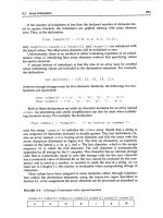
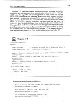
Figure 17.6 Chaos?
The MATLAB solution x is actually a matrix with three columns (as you can
see from whos). The solution y(t) that we want will be the second column,
so to plot it by itself use the command
plot(t,x(:,2),’g’)
Then keep the graph on the axes with the command hold.
Now we can see the effect of changing the initial values. Let’s just change the
initial value of x(0), from −2to−2.04—that’s a change of only 2 percent, and
in only one of the three initial values. The following commands will do this, solve
the DEs, and plot the new graph of y(t) (in a different color):
x0 = [-2.04 -3.5 21];
[t, x] = ode45(@lorenz, [0 10], x0);
plot(t,x(:,2),’r’)

You should see (Figure 17.6) that the two graphs are practically indistinguish-
able until t is about 1.5. The discrepancy grows quite gradually, until t reaches
about 6, when the solutions suddenly and shockingly flip over in opposite direc-
tions. As t increases further, the new solution bears no resemblance to the
old one.
Now solve the system (17.12)–(17.14) with the original initial values using
ode23 this time:
x0 = [-2 -3.5 21];
[t,x] = ode23(@lorenz, [0 10], x0);
378
Ch17-H8417 5/1/2007 11: 45 page 379
17 Introduction to numerical methods
Plot the graph of y(t) only—x(:,2)—and then superimpose the ode45 solution
with the same initial values (in a different color).
A strange thing happens—the solutions begin to deviate wildly for t > 1.5! The
initial conditions are the same—the only difference is the order of the Runge-
Kutta method.
Finally solve the system with ode23s and superimpose the solution. (The s
stands for ‘stiff’. For a stiff DE, solutions can change on a time scale that is
very short compared to the interval of integration.) The ode45 and ode23s
solutions only start to diverge at t > 5.
The explanation is that ode23, ode23s and ode45 all have numerical inaccura-
cies (if one could compare them with the exact solution—which incidentally can’t
be found). However, the numerical inaccuracies are different in the three cases.
This difference has the same effect as starting the numerical solution with very
slightly different initial values.
How do we ever know when we have the ‘right’ numerical solution? Well, we
don’t—the best we can do is increase the accuracy of the numerical method
until no further wild changes occur over the interval of interest. So in our exam-
ple we can only be pretty sure of the solution for t < 5 (using ode23s or ode45).

If that’s not good enough, you have to find a more accurate DE solver.
So beware: ‘chaotic’ DEs are very tricky to solve!
Incidentally, if you want to see the famous ‘butterfly’ picture of chaos, just plot
x against z as time increases (the resulting graph is called a phase plane plot).
The following command will do the trick:
plot(x(:,1), x(:,3))
What you will see is a static 2-D projection of the trajectory, i.e. the solution
developing in time. Demos in the MATLAB Launch Pad include an example which
enables you to see the trajectory evolving dynamically in 3-D (Demos: Graphics:
Lorenz attractor animation).
17.6.3 Passing additional parameters to an ODE solver
In the above examples of the MATLAB ODE solvers the coefficients in the right-
hand sides of the DEs (e.g. the value 28 in Equation (17.13)) have all been
379
Ch17-H8417 5/1/2007 11: 45 page 380
Essential MATLAB for Engineers and Scientists
0
20
40
60
80
100
Population size
120
0246
Time
(a)
(b)
810
Figure 17.7 Lotka-Volterra model: (a) predator; (b) prey

constants. In a real modeling situation, you will most likely want to change
such coefficients frequently. To avoid having to edit the function files each time
you want to change a coefficient, you can pass the coefficients as additional
parameters to the ODE solver, which in turn passes them to the DE function.
To see how this may be done, consider the Lotka-Volterra predator-prey model:
dx/dt = px −qxy (17.15)
dy/dt = rxy −sy, (17.16)
where x(t) and y(t) are the prey and predator population sizes at time t, and p,
q, r and s are biologically determined parameters. For this example, we take
p =0.4, q =0.04, r =0.02, s =2, x(0) =105 and y(0) =8.
First, write a function M-file, volterra.m as follows:
function f = volterra(t, x, p, q, r, s)
f = zeros(2,1);
f(1) = p*x(1) - q*x(1)*x(2);
f(2) = r*x(1)*x(2) - s*x(2);
Then enter the following statements in the Command Window, which generate
the characteristically oscillating graphs in Figure 17.7:
380
Ch17-H8417 5/1/2007 11: 45 page 381
17 Introduction to numerical methods
p = 0.4; q = 0.04; r = 0.02;s=2;
[t,x] = ode23(@volterra,[0 10],[105; 8],[],p,q,r,s);
plot(t, x)
Note:
➤
The additional parameters (p, q, r and s) have to follow the fourth input
argument (options—see help) of the ODE solver. If no options have been
set (as in our case), use [] as a placeholder for the options parameter.
You can now change the coefficients from the Command Window and get a new
solution, without editing the function file.

17.7 A partial differential equation
The numerical solution of partial differential equations (PDEs) is a vast sub-
ject, which is beyond the scope of this book. However, a class of PDEs called
parabolic often lead to solutions in terms of sparse matrices, which were
mentioned briefly in Chapter 16. One such example is considered in this section.
17.7.1 Heat conduction
The conduction of heat along a thin uniform rod may be modeled by the partial
differential equation
∂u
∂t
=
∂
2
u
∂x
2
, (17.17)
where u(x, t) is the temperature distribution a distance x from one end of the
rod at time t, and assuming that no heat is lost from the rod along its length.
Half the battle in solving PDEs is mastering the notation. We set up a rectangular
grid, with step-lengths of h and k in the x and t directions respectively. A general
point on the grid has coordinates x
i
=ih, y
j
=jk. A concise notation for u(x, t)at
x
i
, y
j

is then simply u
i,j
.
Truncated Taylor series may then be used to approximate the PDE by a finite dif-
ference scheme. The left-hand side of Equation (17.17) is usually approximated
by a forward difference:
∂u
∂t
=
u
i,j+1
−u
i,j
k
381
Ch17-H8417 5/1/2007 11: 45 page 382
Essential MATLAB for Engineers and Scientists
One way of approximating the right-hand side of Equation (17.17) is by the
scheme
∂
2
u
∂x
2
=
u
i+1,j
−2u
i,j
+u

i−1,j
h
2
. (17.18)
This leads to a scheme, which although easy to compute, is only conditionally
stable.
If however we replace the right-hand side of the scheme in Equation (17.18)
by the mean of the finite difference approximation on the jth and (j +1)th time
rows, we get (after a certain amount of algebra!) the following scheme for
Equation (17.17):
−ru
i−1,j+1
+(2+2r)u
i,j+1
−ru
i+1,j+1
= ru
i−1,j
+(2−2r)u
i,j
+ru
i+1,j
, (17.19)
where r =k/h
2
. This is known as the Crank-Nicolson implicit method, since it
involves the solution of a system of simultaneous equations, as we shall see.
To illustrate the method numerically, let’s suppose that the rod has a length of
1 unit, and that its ends are in contact with blocks of ice, i.e. the boundary
conditions are

u(0, t) = u(1, t) = 0. (17.20)
Suppose also that the initial temperature (initial condition)is
u(x,0)=

2x,0≤ x ≤ 1/2,
2(1 −x), 1/2 ≤ x ≤ 1.
(17.21)
(This situation could come about by heating the center of the rod for a long
time, with the ends kept in contact with the ice, removing the heat source at
time t =0.) This particular problem has symmetry about the line x =1/2; we
exploit this now in finding the solution.
If we take h =0.1 and k =0.01, we will have r =1, and Equation (17.19)
becomes
−u
i−1,j+1
+4u
i,j+1
−u
i+1,j+1
= u
i−1,j
+u
i+1,j
. (17.22)
Putting j =0 in Equation (17.22) generates the following set of equations for
the unknowns u
i,1
(i.e. after one time step k) up to the mid-point of the rod,
which is represented by i =5, i.e. x =ih =0.5. The subscript j =1 has been
382

Ch17-H8417 5/1/2007 11: 45 page 383
17 Introduction to numerical methods
dropped for clarity:
0 +4u
1
−u
2
= 0 +0.4
−u
1
+4u
2
−u
3
= 0.2 +0.6
−u
2
+4u
3
−u
4
= 0.4 +0.8
−u
3
+4u
4
−u
5
= 0.6 +1.0
−u

4
+4u
5
−u
6
= 0.8 +0.8.
Symmetry then allows us to replace u
6
in the last equation by u
4
. These
equations can be written in matrix form as
⎡
⎢
⎢
⎢
⎢
⎢
⎣
4 −1000
−14−100
0 −14−10
00−14−1
000−24
⎤
⎥
⎥
⎥
⎥
⎥

⎦
⎡
⎢
⎢
⎢
⎢
⎢
⎣
u
1
u
2
u
3
u
4
u
5
⎤
⎥
⎥
⎥
⎥
⎥
⎦
=
⎡
⎢
⎢
⎢

⎢
⎢
⎣
0.4
0.8
1.2
1.6
1.6
⎤
⎥
⎥
⎥
⎥
⎥
⎦
. (17.23)
The matrix (A) on the left of Equations (17.23) is known as a tridiagonal matrix.
Having solved for the u
i,1
we can then put j =1 in Equation (17.22) and proceed
to solve for the u
i,2
, and so on. The system (17.23) can of course be solved
directly in MATLAB with the left division operator. In the script below, the general
form of Equations (17.23) is taken as
Av = g. (17.24)
Care needs to be taken when constructing the matrix A. The following notation
is often used:
A =
⎡

⎢
⎢
⎢
⎢
⎢
⎢
⎢
⎣
b
1
c
1
a
2
b
2
c
2
a
3
b
3
c
3

a
n−1
b
n−1
c

n−1
a
n
b
n
⎤
⎥
⎥
⎥
⎥
⎥
⎥
⎥
⎦
.
A is an example of a sparse matrix (see Chapter 16).
The script below implements the general Crank-Nicolson scheme of Equation
(17.19) to solve this particular problem over 10 time steps of k =0.01. The
step-length is specified by h =1/(2n) because of symmetry. r is therefore not
restricted to the value 1, although it takes this value here. The script exploits
the sparsity of A by using the sparse function.
383
Ch17-H8417 5/1/2007 11: 45 page 384
Essential MATLAB for Engineers and Scientists
format compact
n=5;
k = 0.01;
h = 1 / (2 * n); % symmetry assumed
r=k/hˆ2;
% set up the (sparse) matrix A

b = sparse(1:n, 1:n, 2+2*r, n, n); % b(1) b(n)
c = sparse(1:n-1, 2:n, -r, n, n); % c(1) c(n-1)
a = sparse(2:n, 1:n-1, -r, n, n); % a(2)
A=a+b+c;
A(n, n-1) = -2 * r; % symmetry: a(n)
full(A) %
disp(’ ’)
u0 = 0; % boundary condition (Eq 19.20)
u = 2*h*[1:n] % initial conditions (Eq 19.21)
u(n+1) = u(n-1); % symmetry
disp([0 u(1:n)])
for t = k*[1:10]
g=r*([u0 u(1:n-1)] + u(2:n+1))
+(2-2*r)*u(1:n);
% Eq 19.19
v=A\g’; % Eq 19.24
disp([t v’])
u(1:n) = v;
u(n+1) = u(n-1); % symmetry
end
Note:
➤
to preserve consistency between the formal subscripts of Equation (17.19)
etc. and MATLAB subscripts, u
0
(the boundary value) is represented by the
scalar u0.
In the following output the first column is time, and subsequent columns are
the solutions at intervals of h along the rod:
0 0.2000 0.4000 0.6000 0.8000 1.0000

0.0100 0.1989 0.3956 0.5834 0.7381 0.7691
0.0200 0.1936 0.3789 0.5397 0.6461 0.6921

0.1000 0.0948 0.1803 0.2482 0.2918 0.3069
MATLAB has some built-in PDE solvers. See Using MATLAB: Mathematics:
Differential Equations: Partial Differential Equations.
384
Ch17-H8417 5/1/2007 11: 45 page 385
17 Introduction to numerical methods
0
0
10
20
30
40
50
60
70
80
90
100
y(x)
20 40 60 80 100
x
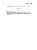
Figure 17.8 A cubic polynomial fit
17.8 Other numerical methods
The ODEs considered earlier in this chapter are all initial value problems.
For boundary value problem solvers, see Using MATLAB: Mathematics:
Differential Equations: Boundary Value Problems for ODEs.
MATLAB has a large number of functions for handling other numerical proce-

dures, such as curve fitting, correlation, interpolation, minimization, filtering
and convolution, and (fast) Fourier transforms. Consult Using MATLAB: Math-
ematics: Polynomials and Interpolation and Data Analysis and Statistics.
Here’s an example of curve fitting. The following script enables you to plot data
points interactively. When you have finished plotting points (signified when the
x coordinates of your last two points differ by less than 2 in absolute value) a
cubic polynomial is fitted and drawn (see Figure 17.8).
% Interactive script to fit a cubic to data points
clf
hold on
axis([0 100 0 100]);
385
Ch17-H8417 5/1/2007 11: 45 page 386
Essential MATLAB for Engineers and Scientists
diff = 10;
xold = 68;
i=0;
xp = zeros(1); % data points
yp = zeros(1);
while diff > 2
[a b] = ginput(1);
diff = abs(a - xold);
if diff > 2
i=i+1;
xp(i) = a;
yp(i) = b;
xold = a;
plot(a, b, ’ok’)
end
end

p = polyfit(xp, yp, 3 );
x = 0:0.1:xp(length(xp));
y= p(1)*x.ˆ3 + p(2)*x.ˆ2 + p(3)*x + p(4);
plot(x,y), title( ’cubic polynomial fit’),
ylabel(’y(x)’), xlabel(’x’)
hold off
Polynomial fitting may also be done interactively in a figure window, with Tools
-> Basic Fitting.
Summary
➤
A numerical method is an approximate computer method for solving a mathematical
problem which often has no analytical solution.
➤
A numerical method is subject to two distinct types of error: rounding error in the
computer solution, and truncation error, where an infinite mathematical process, like
taking a limit, is approximated by a finite process.
➤
MATLAB has a large number of useful functions for handling numerical methods.
EXERCISES
17.1 Use Newton’s method in a script to solve the following (you may have to
experiment a bit with the starting values). Check all your answers with fzero.
Check the answers involving polynomial equations with roots.
386
Ch17-H8417 5/1/2007 11: 45 page 387
17 Introduction to numerical methods
Hint: Use fplot to get an idea of where the roots are, e.g.
fplot(’xˆ3-8*xˆ2+17*x-10’, [0 3])
The Zoom feature also helps. In the figure window select the Zoom In button
(magnifying glass) and click on the part of the graph you want to magnify.
(a) x

4
−x =10 (two real roots and two complex roots)
(b) e
−x
= sin x (infinitely many roots)
(c) x
3
−8x
2
+17x −10=0 (three real roots)
(d) log x = cos x
(e) x
4
−5x
3
−12x
2
+76x −79=0 (four real roots)
17.2 Use the Bisection method to find the square root of 2, taking 1 and 2 as initial
values of x
L
and x
R
. Continue bisecting until the maximum error is less than
0.05 (use Inequality (17.2) of Section 17.1 to determine how many bisections
are needed).
17.3 Use the Trapezoidal rule to evaluate

4
0

x
2
dx, using a step-length of h =1.
17.4 A human population of 1000 at time t =0 grows at a rate given by
dN/dt =aN,
where a =0.025 per person per year. Use Euler’s method to project the
population over the next 30 years, working in steps of (a) h =2 years, (b) h =1
year and (c) h =0.5 years. Compare your answers with the exact mathematical
solution.
17.5 Write a function file euler.m which starts with the line
function [t, n] = euler(a, b, dt)
and which uses Euler’s method to solve the bacteria growth DE (17.8). Use it in
a script to compare the Euler solutions for dt =0.5 and 0.05 with the exact
solution. Try to get your output looking like this:
time dt = 0.5 dt = 0.05 exact
0 1000.00 1000.00 1000.00
0.50 1400.00 1480.24 1491.82
1.00 1960.00 2191.12 2225.54

5.00 28925.47 50504.95 54598.15
17.6 The basic equation for modeling radioactive decay is
dx/dt =−rx,
387
Ch17-H8417 5/1/2007 11: 45 page 388
Essential MATLAB for Engineers and Scientists
where x is the amount of the radioactive substance at time t, and r is the
decay rate.
Some radioactive substances decay into other radioactive substances, which
in turn also decay. For example, Strontium 92 (r
1

=0.256 per hr) decays into
Yttrium 92 (r
2
=0.127 per hr), which in turn decays into Zirconium. Write down
a pair of differential equations for Strontium and Yttrium to describe what is
happening.
Starting at t =0 with 5 ×10
26
atoms of Strontium 92 and none of Yttrium, use
the Runge-Kutta method (ode23) to solve the equations up to t =8 hours in
steps of 1/3 hr. Also use Euler’s method for the same problem, and compare
your results.
17.7 The springbok (a species of small buck, not rugby players!) population x(t)inthe
Kruger National Park in South Africa may be modeled by the equation
dx/dt = (r − bx sin at)x,
where r, b, and a are constants. Write a program which reads values for r, b,
and a, and initial values for x and t, and which uses Euler’s method to compute
the impala population at monthly intervals over a period of two years.
17.8 The luminous efficiency (ratio of the energy in the visible spectrum to the total
energy) of a black body radiator may be expressed as a percentage by the
formula
E = 64.77T
−4

7×10
−5
4×10
−5
x
−5

(e
1.432/Tx
−1)
−1
dx,
where T is the absolute temperature in degrees Kelvin, x is the wavelength in
cm, and the range of integration is over the visible spectrum.
Write a general function simp(fn, a, b, h) to implement Simpson’s rule as
given in Equation (17.4).
Taking T =3500
◦
K, use simp to compute E, firstly with 10 intervals (n =5), and
then with 20 intervals (n =10), and compare your results.
(Answers: 14.512725% for n =5; 14.512667% for n =10)
17.9 Van der Pol’s equation is a second-order nonlinear differential equation which
may be expressed as two first-order equations as follows:
dx
1
/dt = x
2
dx
2
/dt = (1 −x
2
1
)x
2
−b
2
x

1
.
388
Ch17-H8417 5/1/2007 11: 45 page 389
17 Introduction to numerical methods
The solution of this system has a stable limit cycle, which means that if you plot
the phase trajectory of the solution (the plot of x
1
against x
2
) starting at any
point in the positive x
1
–x
2
plane, it always moves continuously into the same
−3 −2
−2
−2.5
−1.5
−1
−0.5
0
0.5
1
1.5
2
2.5
−1
0123

Figure 17.9 A trajectory of Van der Pol’s equation
closed loop. Use ode23 to solve this system numerically, for x
1
(0) =0, and
x
2
(0) =1. Draw some phase trajectories for b =1 and  ranging between 0.01
and 1.0. Figure 17.9 shows you what to expect.
389
App-A-H8417 5/1/2007 11: 46 page 390
Appendix A
Syntax quick reference
This appendix gives examples of the most commonly used MATLAB syntax in this book.
A.1 Expressions
x=2ˆ(2*3)/4;
x=A\b; %solution of linear equations
a==0&b<0 %aequals 0 AND b less than 0
a˜=4|b>0 %anotequal to 4 OR b greater than 0
A.2 Function M-files
function y = f(x) % save as f.m
% comment for help
function [out1, out2] = plonk(in1, in2, in3) % save as plonk.m
% Three input arguments, two outputs

function junk % no input/output arguments; save as junk.m
[t, x] = ode45(@lorenz, [0 10], x0); % function handle with @
A.3 Graphics
plot(x, y), grid % plots vector y against vector x on a grid
plot(x, y, ’b ’) % plots a blue dashed line
App-A-H8417 5/1/2007 11: 46 page 391

Appendix A Syntax quick reference
plot(x, y, ’go’) % plots green circles
plot(y) % if y is a vector plots elements against row numbers
% if y is a matrix, plots columns against row numbers
plot(x1, y1, x2, y2) % plots y1 against x1 and
y2 against x2 on same graph
semilogy(x, y) % uses a log10 scale for y
polar(theta, r) % generates a polar plot
A.4 if and switch
if condition
statement % executed if condition true
end;
if condition
statement1 % executed if condition true
else
statement2 % executed if condition false
end;
if a == 0 % test for equality
x=-c/b;
else
x = -b / (2*a);
end;
if condition1 % jumps off ladder at first true condition
statement1
elseif condition2 % elseif one word!
statement2
elseif condition3
statement3

else

statementE
end;
if condition statement1, else statement2, end % command line
391
App-A-H8417 5/1/2007 11: 46 page 392
Essential MATLAB for Engineers and Scientists
switch lower(expr) % expr is string or scalar
case {’linear’,’bilinear’}
disp(’Method is linear’)
case ’cubic’
disp(’Method is cubic’)
case ’nearest’
disp(’Method is nearest’)
otherwise
disp(’Unknown method.’)
end
A.5 for and while
for i = 1:n % repeats statements n times
statements
end;
for i = 1:3:8 % i takes values 1, 4, 7

end;
for i = 5:-2:0 % i takes values 5, 3, 1

end;
fori=v %index i takes on each element of vector v
statements
end;
forv=a %index v takes on each column of matrix a

statements
end;
for i = 1:n, statements, end % command line version
try,
statements,
catch,
statements,
end
while condition % repeats statements while condition is true
statements
end;
while condition statements, end % command line version
392
App-A-H8417 5/1/2007 11: 46 page 393
Appendix A Syntax quick reference
A.6 Input/output
disp( x )
disp( ’Hello there’ )
disp([a b]) % two scalars on one line
disp([x’ y’]) % two columns (vectors x and y must be same length)
disp( [’The answer is ’, num2str(x)] )
fprintf( ’\n’ ) % new line
fprintf( ’%5.1f\n’, 1.23 ) % **1.2
fprintf( ’%12.2e\n’, 0.123 ) % ***1.23e-001
fprintf( ’%4.0f and %7.2f\n’, 12.34, -5.6789 )
% **12 and **-5.68
fprintf( ’Answers are: %g %g\n’, x, y ) % matlab decides on format
fprintf( ’%10s\n’, str ) % left-justified string
x = input( ’Enter value of x: ’ )
name = input( ’Enter your name without apostrophes: ’, ’s’ )

A.7 load/save
load filename % retrieves all variables
from binary file filename.mat
load x.dat % imports matrix x from ASCII file x.dat
save filenamexyz %saves x y and z in filename.mat
save
% saves all workspace variables in matlab.mat
save filename x /ascii % saves x in filename
(as ASCII file)
A.8 Vectors and matrices
a(3,:) % third row
a(:,2) % second column
393
App-A-H8417 5/1/2007 11: 46 page 394
Essential MATLAB for Engineers and Scientists
v(1:2:9) % every second element from 1 to 9
v([245])=[] %removes second, fourth and fifth elements
v(logical([01010])) % second and fourth elements only
v’ % transpose
394
App-B-H8417 5/1/2007 11: 47 page 395
Appendix B
Operators
Table B.1 Operator precedence (see Help on operator precedence)
Precedence Operators
1. ()
2. ˆ.ˆ’.’(pure transpose)
3. + (unary plus) - (unary minus) ˜ (NOT)
4. */\ .* ./ .\
5. + (addition) - (subtraction)

6. :
7. ><>=<===˜=
8. & (AND)
9. |(OR)
App-C-H8417 5/1/2007 11: 47 page 396
Appendix C
Command and functionquick
reference
This appendix is not exhaustive; it lists most of the MATLAB commands and functions used
in the text, as well as a few more.
For a complete list by category (with links to detailed descriptions) see the online
documentation MATLAB: Reference: MATLAB Function Reference: Functions by Category.
The command help by itself displays a list of all the function categories (each in its own
directory):
matlab\general - General purpose commands.
matlab\ops - Operators and special characters.
matlab\lang - Programming language constructs.
matlab\elmat - Elementary matrices and matrix
manipulation.
matlab\elfun - Elementary math functions.
matlab\specfun - Specialized math functions.
matlab\matfun - Matrix functions - numerical
linear algebra.
matlab\datafun - Data analysis and Fourier
transforms.
matlab\audio - Audio support.
matlab\polyfun - Interpolation and polynomials.
matlab\funfun - Function functions and ODE
solvers.
matlab\sparfun - Sparse matrices.

matlab\graph2d - Two dimensional graphs.
matlab\graph3d - Three dimensional graphs.
matlab\specgraph - Specialized graphs.
matlab\graphics - Handle Graphics.
matlab\uitools - Graphical user interface tools.
matlab\strfun - Character strings.
App-C-H8417 5/1/2007 11: 47 page 397
Appendix C Command and functionquick reference
matlab\iofun - File input/output.
matlab\timefun - Time and dates.
matlab\datatypes - Data types and structures.
matlab\verctrl - Version control.
matlab\winfun - Windows Operating System
matlab\DDE/ActiveX) - Interface Files
matlab\demos - Examples and demonstrations.
toolbox\local - Preferences.
MATLABR12\work - (No table of contents file)
For more help on directory/topic, type "help topic".
C.1 General purpose commands
C.1.1 Managing commands
demo Run demos
help Online help
helpwin Display categories of functions with links to each category
lookfor Keyword search through help entries
type List M-file
what Directory listing of M- and MAT-files
which Locate functions and files
C.1.2 Managing variables and the workspace
clear Clear variables and functions from memory
disp Display matrix or text

length Length of a vector
load Retrieve variables from disk
save Save workspace variables to disk
size Array dimensions
who, whos List variables in the workspace
C.1.3 Files and the operating system
beep Produce a beep sound
cd Change current working directory
397
App-C-H8417 5/1/2007 11: 47 page 398
Essential MATLAB for Engineers and Scientists
delete Delete file
diary Save text of MATLAB session
dir Directory listing
edit Edit an M-file
! Execute operating system command
C.1.4 Controlling the Command Window
clc Clear Command Window
echo Echo commands in script
format Set output format for disp
home Send cursor home
more Control paged output
C.1.5 Starting and quitting MATLAB
exit Terminate MATLAB
quit Terminate MATLAB
startup M-file executed when MATLAB starts
C.2 Logical functions
all True if all elements of vector are true (non-zero)
any True if any element of vector is true
exist Check if variable or file exists

find Find indices of non-zero elements
is* Detect various states
logical Convert numeric values to logical
C.3 Language constructs and debugging
C.3.1 MATLAB as a programming language
error Display error message
eval Interpret string containing MATLAB expression
398
App-C-H8417 5/1/2007 11: 47 page 399
Appendix C Command and functionquick reference
feval Function evaluation
for Repeat statements a specific number of times
global Define global variable
if Conditionally execute statements
persistent Define persistent variable
switch Switch among several cases
try Begin try block
while Repeat statements conditionally
C.3.2 Interactive input
input Prompt user for input
keyboard Invoke keyboard as a script file
menu Generate menu of choices for user input
pause Wait for user response
C.4 Matrices and matrix manipulation
C.4.1 Elementary matrices
eye Identity matrix
linspace Vector with linearly spaced elements
ones Matrix of ones
rand Uniformly distributed random numbers and arrays
randn Normally distributed random numbers and arrays

zeros Matrix of zeros
: (colon) Vector with regularly spaced elements
C.4.2 Special variables and constants
ans Most recent answer
eps Floating point relative accuracy
iorj
√
−1
Inf Infinity
NaN Not-a-Number
nargin, nargout Number of actual function arguments
pi 3.14159 26535 897 …
realmax Largest positive floating point number
realmin Smallest positive floating point number
varargin, varargout Pass or return variable numbers of arguments
399
App-C-H8417 5/1/2007 11: 47 page 400
Essential MATLAB for Engineers and Scientists
C.4.3 Time and date
calendar Calendar
clock Wall clock (complete date and time)
date You’d never guess
etime Elapsed time
tic, toc Stopwatch
weekday Day of the week
C.4.4 Matrix manipulation
cat Concatenate arrays
diag Create or extract diagonal
fliplr Flip in left/right direction
flipud Flip in up/down direction

repmat Replicate and tile an array
reshape Change shape
rot90 Rotate 90
◦
tril Extract lower tridiagonal part
triu Extract upper tridiagonal part
C.4.5 Specialized matrices
gallery Test matrices
hilb Hilbert matrix
magic Magic square
pascal Pascal matrix
wilkinson Wilkinson’s eigenvalue test matrix
C.5 Mathematical functions
abs Absolute value
acos, acosh Inverse cosine and inverse hyperbolic cosine
acot, acoth Inverse cotangent and inverse hyperbolic cotangent
acsc, acsch Inverse cosecant and inverse hyperbolic cosecant
angle Phase angle
asec, asech Inverse secant and inverse hyperbolic secant
400
App-C-H8417 5/1/2007 11: 47 page 401
Appendix C Command and functionquick reference
asin, asinh Inverse sine and inverse hyperbolic sine
atan, atanh Inverse tangent (two quadrant) and inverse hyperbolic
tangent
atan2 Inverse tangent (four quadrant)
bessel Bessel function
ceil Round up
conj Complex conjugate
cos, cosh Cosine and hyperbolic cosine

cot, coth Cotangent and hyperbolic cotangent
csc, csch Cosecant and hyperbolic cosecant
erf Error function
exp Exponential
fix Round toward zero
floor Round down
gamma Gamma function
imag Imaginary part
log Natural logarithm
log2 Dissect floating point numbers into exponent and
mantissa
log10 Common logarithm
mod Modulus (signed remainder after division)
rat Rational approximation
real Real part
rem Remainder after division
round Round toward nearest integer
sec, sech Secant and hyperbolic secant
sign Signum function
sin, sinh Sine and hyperbolic sine
sqrt Square root =-16pt =8pt
tan, tanh Tangent and hyperbolic tangent
C.6 Matrix functions
det Determinant
eig Eigenvalues and eigenvectors
expm Matrix exponential
inv Matrix inverse
poly Characteristic polynomial
rank Number of linearly independent rows or columns
rcond Condition estimator

trace Sum of diagonal elements
{}\ and / Linear equation solution
401