Báo cáo sinh học: "Association of repeatedly measured intermediate risk factors for complex diseases with high dimensional SNP data." pot

Waaijenborg and Zwinderman Algorithms for Molecular Biology 2010, 5:17
/>Open Access
RESEARCH
© 2010 Waaijenborg and Zwinderman; licensee BioMed Central Ltd. This is an Open Access article distributed under the terms of the
Creative Commons Attribution License ( which permits unrestricted use, distribution,
and reproduction in any medium, provided the original work is properly cited.
Research
Association of repeatedly measured intermediate
risk factors for complex diseases with high
dimensional SNP data
Sandra Waaijenborg and Aeilko H Zwinderman*
Abstract
Background: The causes of complex diseases are difficult to grasp since many different factors play a role in their
onset. To find a common genetic background, many of the existing studies divide their population into controls and
cases; a classification that is likely to cause heterogeneity within the two groups. Rather than dividing the study
population into cases and controls, it is better to identify the phenotype of a complex disease by a set of intermediate
risk factors. But these risk factors often vary over time and are therefore repeatedly measured.
Results: We introduce a method to associate multiple repeatedly measured intermediate risk factors with a high
dimensional set of single nucleotide polymorphisms (SNPs). Via a two-step approach, we summarized the time courses
of each individual and, secondly apply these to penalized nonlinear canonical correlation analysis to obtain sparse
results.
Conclusions: Application of this method to two datasets which study the genetic background of cardiovascular
diseases, show that compared to progression over time, mainly the constant levels in time are associated with sets of
SNPs.
Background
Among the examples of complex diseases, several of the
major (lethal) diseases in the western world can be found,
including cancer, cardiovascular diseases and diabetes.
Increasing our understanding of the underlying genetic
background is an important step that can contribute in
the development of early detection and treatment of such

diseases. While many of the existing studies have divided
their study population into controls and cases, this classi-
fication is likely to cause heterogeneity within the two
groups. This heterogeneity is caused by the complexity of
gene regulation, as well as many extra- and intracellular
factors; the same disease can be caused by (a combination
of) different pathogenetic pathways, this is referred to as
phenogenetic equivalence. Due to this heterogeneity, the
genetic markers responsible for, or involved in the onset
and progression of the disease are difficult to identify [1].
Moreover, the risk of misclassification is increased if the
time of onset of the disease varies.
In order to overcome these problems, rather than divid-
ing the study population into cases and controls, it is
preferable to identify the phenotype of a complex disease
by a set of intermediate risk factors. Because of the high
diversity of pathogenetic causes that can lead to a com-
plex disease, such intermediate risk factors are likely to
have a much stronger relationship with the measured
genetic markers. Intermediate risk factors can come in a
number of varieties, as broad as the whole gene expres-
sion pattern of an individual up to as specific as a set of
phenotypic biomarkers chosen based upon prior knowl-
edge of the diseases, e.g., lipid profiles as possible risk fac-
tors for cardiovascular diseases. These risk factors often
vary over time and are therefore repeatedly measured.
In recent studies we have used penalized canonical cor-
relation analysis (PCCA) to find associations between
two sets of variables, one containing phenotypic and the
other containing genomic data [2,3]. PCCA penalizes the

two datasets such that it finds a linear combination of a
selection of variables in one set that maximally correlates
* Correspondence:
1
Department of Clinical Epidemiology, Biostatistics and Bioinformatics,
Academic Medical Center, University of Amsterdam, Meibergdreef 9, 1100 DD
Amsterdam, the Netherlands
Waaijenborg and Zwinderman Algorithms for Molecular Biology 2010, 5:17
/>Page 2 of 13
with a linear combination of a selection of variables in the
other set; thereby making the results more interpretable.
Highly correlated variables, caused by eg. co-expressed
genes, are grouped into the same results.
Although canonical correlation analysis accounts for
the correlation between variables within the same vari-
able set, CCA is not capable of taking advantage of the
simple covariance structure of the longitudinal data. Our
goal was to provide biological and medical researchers
with a much needed tool to investigate the progression of
complex diseases in relationship to the genetic profiles of
the patients. To achieve this, we introduce a two-step
approach: first we summarize each time course of each
individual and, secondly, we apply penalized canonical
correlation analysis, where the uncertainty of the sum-
mary estimates is taken into account by using weighted-
least squares. Additionally, optimal scaling is applied
such that qualitative variables can be used within the
PCCA, resulting in penalized nonlinear CCA (PNCCA)
[3]; e.g., for transforming single nucleotide polymor-
phisms (SNPs) into continuous variables such that they

capture the measurement characteristics of the SNPs. By
adapting these approaches, we are able to extract groups
of categorical genetic markers that have a high associa-
tion with multiple repeatedly measured intermediate risk
factors.
To illustrate PNCCA, this method was applied to two
datasets. The first dataset is part of the Framingham
Heart Study
,
which contains information about repeatedly measured
common characteristics that contribute to cardiovascular
diseases (CVD), together with genetic data of about
50,000 SNPs. These data were provided for participants
to the genetic analysis workshop 16 (GAW16). The sec-
ond dataset is the REGRESS dataset [4], which contains
information about lipid profiles together with about 100
SNPs located in candidate genes. By applying PCCA, we
were able to extract groups of SNPs which were highly
associated with a set of repeatedly measured intermediate
risk factors. Cross-validation was used to determine the
optimal number of SNPs within the selected SNP clus-
ters.
Results and Discussion
Framingham heart study
The Framingham heart study was performed to study
common characteristics that contribute to cardiovascular
diseases (CVD). Besides information about these risk fac-
tors, the study contains information about genetic data of
about 50,000 single nucleotide polymorphisms (SNPs).
Risk factors were measured from the start of the study in

1948 up to four times, every 7 to 12 years. Three genera-
tions were followed, however, to have consistent mea-
surements, only the individuals of the second generation
were included in this study. The data of the Framingham
heart study were provided for participants to the genetic
analysis workshop 16 (GAW grant, R01 GM031575).
We considered the measurements of LDL cholesterol
(mg/dl), HDL cholesterol (mg/dl), triglycerides (mg/dl),
blood glucose (mg/dl), systolic and diastolic blood pres-
sure and body mass index; each measured up to 4 times
(in fasting blood samples). LDL cholesterol was estimated
using the Friedewald formula: LDL cholesterol = total
cholesterol - HDL cholesterol - 0.2*triglycerides. Further-
more, we considered the data of the affymetrix 50 K chip
containing about 50,000 SNPs.
The offspring generation consists of 2,583 individuals
over the age of 17, of which 157 suffered from a coronary
heart disease (of which 2 before the beginning of the
study). From this data 3 individuals had a negative LDL
cholesterol level and were therefore removed from the
data, together with 27 individuals who had less than 2
observations for one or more of the 7 intermediate risk
factors. 7 individuals were removed because they were
missing more than 5% of their genetic data. Monomor-
phic SNPs and SNPs with a missing percentage of 5% or
more were deleted from further analysis, remaining miss-
ing data were randomly imputed based only on the mar-
ginal distribution of the SNP in all other individuals.
Because our primary interest concerned common SNP
variants, we therefore grouped SNP classes with less than

1% observations, with its neighboring SNP class; i.e., we
grouped homozygotes of the rare allele together with the
heterozygotes. This resulted in a dataset consisting of
2,546 individuals, 7 intermediate risk factors and 37,931
SNPs.
Penalized nonlinear canonical correlation analysis was
used to identify SNPs that are associated with a combina-
tion of intermediate risk factors of cardiovascular dis-
eases. Here for, the data was divided based upon subjects
into two sets; one test set containing 546 subjects and an
estimation set of 2,000 subjects to estimate the weights in
the canonical variates, the transformation functions and
to determine the optimal number of variables within the
SNP dataset.
To remove the dependency within the longitudinal
data, seven models were fitted, one for each of the seven
intermediate risk factors. The individual change pattern
in time of each of the seven intermediate risk factors was
summarized with the best linear unbiased predictions
(BLUP) of the intercept and slope parameters, using the
following mixed effect model:
log y b b age sex trt
se
it i i it it i it
2
00 11 2 3
4
()( )( )=+++× +× +×+
×
ββ β β

β
xx age trt age
iit ititit
×+××+
βε
5
,
Waaijenborg and Zwinderman Algorithms for Molecular Biology 2010, 5:17
/>Page 3 of 13
y
it
represents one of the seven risk factors of individual i
measured at age t, trt
it
the treatment individual i received
at age t and sex
i
the gender of the individual i. In the mod-
els for LDL cholesterol, HDL cholesterol, triglycerides,
blood glucose and BMI, the treatment with cholesterol
lowering medication was used as a covariate. In the mod-
els for systolic and diastolic blood pressure, blood pres-
sure lowering medication was used. Here, trt = 0 stands
for no medication and trt = 1 for pharmacological treat-
ment. The measurements for both age as well as the risk
factors were standardized to have mean zero.
A new dataset was formed, containing the random
intercepts and the random slopes from each individual,
for each of the seven intermediate risk factors. The ran-
dom slopes and random intercepts of the blood glucose

variable had a perfect correlation, indicating no time
effect to be present. Therefore the slope variable of the
blood glucose variable was removed from the newly
obtained dataset, which resulted in a set containing 13
measures (7 random intercepts (b
0i
's) and 6 random
slopes (b
1i
's) (see table 1)) and a weight set with 13
accompanying standard errors.
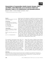
By means of 10-fold cross-validation, the optimal num-
ber of SNP variables was determined for several canoni-
cal variates (see figure 1). As can be seen in figure 1, with
increasing number of selected variables, the difference
between the canonical correlation of the validation and
the training set also increased. For the first canonical
variate pair (figure 1a), the difference between the canon-
ical correlation of the permuted validation set and the
training set was high, indicating that there were associat-
ing SNPs present in the dataset. Adding more variables to
the model did not decrease the difference between valida-
tion and training sets, therefore, the number of important
variables was very small. A model with 1 SNP variables
was optimal, however, to be sure not to miss any impor-
tant SNPs, we built a model containing 5 SNPs. PNCCA
was next performed on the whole estimation dataset,
obtaining 5 SNP variables associated with all the pheno-
typical intermediate risk factors, this resulted in a model
with a canonical correlation of 0.24. The weights and

transformations of this optimal model were applied to the
test set, resulting in a canonical correlation of 0.17. The
loadings (correlations of variables and their respective
canonical variates) and cross-loadings (correlations of
variables with their opposite canonical variate) are given
in tables 1 and 2 for the intermediate risk factors and
selected SNPs, respectively. In figure 2 the transforma-
tions of the selected SNP variables are given, it can be
seen that almost all SNPs had an additive effect, except
for SNP rs9303601, which had a recessive effect.
The first canonical variate pair showed a strong associ-
ation between the HDL intercept and SNP rs3764261,
which is closely located to the CETP gene and has been
reported to be associated with HDL concentrations [5].
The low loadings of the other SNPs show their small con-
tribution to the first canonical variate of the SNP, this
Table 1: Intermediate risk factors of the Framingham heart study.
First canonical variate Second canonical variate
Phenotype Loadings Cross-loadings Loadings Cross-loadings
HDL intercept 0.76 0.18 -0.25 -0.10
HDL slope -0.05 -0.02 0.07 0.03
LDL intercept -0.16 -0.04 -0.12 -0.05
LDL slope -0.07 -0.02 -0.08 -0.03
triglyceride intercept -0.10 -0.03 -0.02 -0.01
triglyceride slope 0.15 0.04 0.11 0.04
blood glucose 0.02 0.01 0.65 0.25
systolic intercept -0.07 -0.01 0.08 0.02
systolic slope -0.11 -0.02 0.08 0.02
diastolic intercept 0.06 0.02 0.13 0.05
diastolic slope -0.11 -0.03 0.16 0.06

BMI intercept -0.05 0.00 0.73 0.30
BMI slope 0.07 0.02 0.71 0.28
The loadings and cross-loadings of the intermediate risk factors within the first and second canonical variate pair.
Waaijenborg and Zwinderman Algorithms for Molecular Biology 2010, 5:17
/>Page 4 of 13
confirmed our results of the optimization step, which
indicated that one SNP would be sufficient. Based on the
loadings and cross-loadings, the canonical variate of the
intermediate risk factors also seems to be constructed of
one variable only, namely the HDL intercept.
Based upon the residual estimation matrix, the second
canonical variate pair was obtained in a similar fashion
via cross-validation. For small numbers of variables the
predictive performance was limited (see figure 1b), which
was represented by the overlap between the results of the
validation and the permutation sets. With larger number
of SNPs (>40) a clearer separation between the validation
and the permutation set appeared, but the difference in
canonical correlation also increased. We therefore chose
to make a model with 40 SNPs.
Penalized CCA was next performed on the whole
(residual) estimation set to obtain a model with 40 SNP
variables associated with all the intermediate risk factors,
this resulted in a model with a canonical correlation of
0.40, and a canonical correlation in the (residual) test set
of 0.02. This shows the importance of the permutation
tests; as we could already see by the overlap between the
validation and the permutation results in figure 1b, the
predictive performance of the model was expected to be
poor as was confirmed by the canonical correlation of the

test set.
Although the loadings and cross-loadings for some of
the SNPs (rs12713027 and rs4494802, both located in the
follicle stimulating hormone receptor) and intermediate
risk factors (blood glucose and BMI) were quite high, no
references could be found to confirm these associations.
Because the second canonical variate pair was hardly
distinguishable from the permutation results, we did not
obtain further variate pairs.
REGRESS data
The Regression Growth Evaluation Statin Study
(REGRESS) [4] was performed to study the effect of 3-
hydroxy-3-methylglutaryl coenzyme A reductase inhibi-
tor pravastatin on the progression and regression of coro-
nary atherosclerosis. 885 male patients, with a serum
cholesterol level between 4 and 8 mmol/l, were random-
ized to either treatment or placebo group. Levels for HDL
cholesterol, LDL cholesterol and triglycerides were mea-
sured repeatedly over time, at baseline (before treatment)
and 2, 4, 6, 12, 18 and 24 months after the beginning of
the treatment. For each patient 144 SNPs in candidate
genes were determined, after removing monomorphic
SNPs and SNPs with more than 20% missing data, 99
SNPs remained and missing data were imputed. Individu-
als without a baseline measurement and individuals with
less than 2 follow-up measurements and/or more than
10% missing SNPs were excluded from the analysis. The
final dataset contained 675 individuals together with 99
SNPs located in candidate genes and 3 intermediate risk
factors.

The dataset was divided into two sets, one estimation
set with 500 subjects and a test set of 175 subjects. To
remove the dependency within the longitudinal data,
Framingham heart study
Figure 1 Framingham heart study. Optimization of the first (a) and second (b) canonical variate, for differing number of SNP variables.
Waaijenborg and Zwinderman Algorithms for Molecular Biology 2010, 5:17
/>Page 5 of 13
Table 2: Selected SNPs in the Framingham heart study.
Chrom Position ID Gene symbol Loadings Cross-loadings
First canonical variate
6 36068368 rs17707331 SLC26A8 0.03 0.10
6 36088099 rs743923 SLC26A8 0.02 0.10
8 62213297 rs17763714 0.02 0.10
16 55550825 rs3764261 near CETP 1.00 0.23
17 39634367 rs9303601 -0.00 0.10
Second canonical variate
1 54388154 rs11576359 CDCP2 0.07 0.09
1 70656428 rs1145920 CTH 0.17 0.10
1 82015671 rs12072054 0.09 0.09
2 28371365 rs4666051 BRE 0.15 0.10
2 33358643 rs2290427 LTBP1 0.11 0.09
2 49052952 rs12713027 FSHR 0.41 0.10
2 49074650 rs4494802 FSHR 0.67 0.14
2 177267412 rs16864244 LOC375295 0.08 0.09
3 122662360 rs669277 POLQ 0.15 0.09
3 122669112 rs532411 POLQ 0.14 0.09
4 178830262 rs13149928 0.19 0.10
5 79069147 rs2278240 CMYA5 0.19 0.10
6 33380833 rs2071888 TAPBP 0.13 0.10
6 42374980 rs4714595 TRERF1 0.06 0.08

6 102197213 rs6925691 GRIK2 0.25 0.11
6 116504475 rs12527159 0.23 0.10
7 116990653 rs213952 CFTR 0.11 0.10
7 129737976 rs2171492 CPA4 0.22 0.10
7 129771213 rs7786598 CPA5 0.27 0.09
7 129772024 rs1532047 CPA5 0.29 0.10
7 137639294 rs410156 0.08 0.09
8 23574003 rs7006278 0.07 0.09
10 71959784 rs2275060 KIAA1274 0.15 0.09
10 81916682 rs1049550 ANXA11 0.18 0.10
11 12036827 rs2403569 0.07 0.08
11 24693192 rs2631439 LUZP2 0.14 0.09
11 33438534 rs2615913 0.20 0.10
11 92329680 rs7936247 0.11 0.09
11 101990763 rs7126560 MMP20 0.23 0.10
11 133808516 rs7949167 0.07 0.08
12 7040597 rs12146727 C1S 0.23 0.10
12 14873619 rs3088190 ART4 0.11 0.09
Waaijenborg and Zwinderman Algorithms for Molecular Biology 2010, 5:17
/>Page 6 of 13
each of the three intermediate risk factors was summa-
rized into two summary measures, a random intercept
and a random slope, using the following mixed effect
model:
y
i0
was the measurement of risk factor y taken at base-
line for patient i; i.e. the time point before medication was
given. trt was either placebo or pravastatin. The measure-
ments for both age as well as the risk factor at time point

zero and the risk factors were standardized to have mean
zero. The random slopes and random intercepts of LDL
cholesterol, HDL cholesterol and triglyceride formed set
Y.
Via 10-fold cross-validation the optimal number of SNP
variables was determined (see figure 3). As can be seen
from figure 3, the optimal number of variables was 5. The
model containing 5 SNPs had a canonical correlation of
0.23 in the whole estimation set and a canonical correla-
tion of -0.04 in the test set. The loadings and cross-load-
ings are given in tables 3 and 4, for the selected SNPs and
risk factors, respectively. All the selected SNPs are
located in the CETP gene, the obtained canonical variate
correlated mostly with the HDL intercept. These results
are quite similar to the results of the Framingham heart
study, where a SNP closely located to the CETP gene
highly associated with the HDL intercept.
The residual matrix for the intermediate risk factors
was determined and while obtaining the second canoni-
cal variate, the SNPs selected in the first canonical variate
were fixed at their optimal transformation. The validation
and permutation results were overlapping (data not
shown), so no further information could be obtained
from this dataset.
Conclusions
We have introduced a new method to associate multiple
repeatedly measured intermediate risk factors with high
dimensional SNP data. In this paper we have chosen to
summarize the longitudinal measures into random inter-
cept and random slopes via mixed-effects models.

Mixed-effects models deal with intra-subject correlation
by allowing random effects in the models, these models
focus on both population-average and individual profiles
by taking the dependency between repeated measures
into account. Due to the high number of possible models,
they can be too restrictive in the assumed change over
time. Further, these models need many assumptions for
the underlying model.
Other techniques to summarize longitudinal profiles,
like area under the curve, average progress, etc., focus
mainly on certain aspects of the response profile, or fail in
the presence of unbalanced data. Often they lose infor-
mation about the variability of the observations within
patients. The pros and cons of summary statistics should
be weighed to come up with the best solution, our deci-
sion to use mixed-effect models was based on the fact
that the data showed a linear trend and because there was
unbalanced data; i.e., unequal number of measurements
for the individuals and the Framingham heart study mea-
surements were not taken at fixed time points.
To make the results more interpretable, we chose only
to penalize the X-side containing the SNPs. The number
of intermediate risk factors was sufficiently small such
that penalizing the number of variables would not
increase the interpretation. While modeling the second
canonical variate pair, a small ridge penalty was added to
the Y-side to overcome the multicollinearity caused by
the removal of the information of the first canonical vari-
ate.
Alternative methods for our two-step approach include

performing penalized CCA without considering the fact
that variables are repeatedly measured. This can be rea-
sonable in the case of clinical studies, where one wants to
see if changes at a certain time point after the beginning
of a treatment are associated with certain risk factors.
However, in observational studies fixed time points are
log y b b time y trt trt
it i i it i i i
2
00 11 2 0 3 4
()( )( )=+++× +×+×+××
ββ βββ
ttime
it it
+
ε
.
13 95455188 rs16951415 UGCGL2 0.13 0.09
14 59141031 rs10483717 RTN1 0.29 0.11
15 64238853 rs4776752 MEGF11 0.15 0.09
16 15548316 rs9930648 C16orf45 0.05 0.08
16 77671528 rs12935535 WWOX 0.11 0.09
17 53939507 rs2302190 MTMR4 0.14 0.10
19 38606005 rs11084731 PEPD 0.29 0.11
22 37171988 rs196084 KCNJ4 0.09 0.09
Selected SNPs within the first and second canonical variate pair, together with their loadings and cross-loadings.
Table 2: Selected SNPs in the Framingham heart study. (Continued)
Waaijenborg and Zwinderman Algorithms for Molecular Biology 2010, 5:17
/>Page 7 of 13
Transformation of the selected SNPs

Figure 2 Transformation of the selected SNPs. Transformation of the selected SNPs in the Framingham heart study.
01 2
-4-202468
Original categories
Transformed values
rs3764261
rs17763714
rs743923
rs9303601
rs17707331
Table 4: Intermediate risk factors of the REGRESS study.
Phenotype Loadings Cross-loadings
HDL intercept 0.75 0.17
HDL slope -0.14 -0.03
LDL intercept -0.19 -0.03
LDL slope -0.11 -0.03
triglyceride intercept 0.27 0.07
triglyceride slope 0.28 0.07
The loadings and cross-loadings of the intermediate risk factors within the first canonical variate pair.
Waaijenborg and Zwinderman Algorithms for Molecular Biology 2010, 5:17
/>Page 8 of 13
difficult to obtain and getting a matrix without too much
missing data is almost impossible, due to the diversity of
time points at which a measurement can be obtained.
Another option might be to summarize each repeatedly
measured variable and associate them separately with the
SNP data via a regression model in combination with the
elastic net and optimal scaling. However, this method
does not take the dependency between the intermediate
risk factors into account and moreover, it can transform

each SNP variable differently; which makes it difficult to
integrate the results of the different regression models.
The residual matrix of the X-side, achieved by fixing
the transformed variables in their primary transformed
optimal form, was optional. In studies with small num-
bers of SNP variables, like in the case of the REGRESS
study, fixation is preferred to overcome the same variable
to be optimized twice. For studies like the Framingham
heart study, fixation is not necessary, since there is almost
no overlap between the selected SNPs in succeeding
canonical variate pairs.
Strikingly, both studies showed an association between
SNPs located near or in the CETP gene and the HDL
intercept. Neither of the datasets could find other associ-
ations, which could be explained by the absence of impor-
tant (environmental) factors, or by the fact that SNP
effect is more complicated and more complex models are
necessary to model this effect. The results in both studies
show that the random intercepts get the highest loadings
and cross-loading, while the random slopes seem to be
less associated with the selected SNPs. This could indi-
cate that individuals average values are to some extent
genetically determined, while the changes over time are
influenced by other factors, e.g. environmental factors.
The selected SNPs within the first canonical variate
pairs are consistent with results found in literature [6],
however, the reproducibility is quite low, especially in the
REGRESS study where canonical correlation of the test
set came close to zero. It seems that the bias caused by
univariate soft-thresholding has considerable impact on

the weight estimation and therefore predictive perfor-
mance is quite low, especially in studies where the canon-
ical correlation is already low due to the absence of
important variables. Our method is especially useful as a
primarily tool for gene discovery, such that biologists
have a much smaller subset for deeper exploration, and
not so much as to make predictive models.
Methods
Our focus lies on intermediate risk factors, we assume
that individuals with similar progression-profiles of the
intermediate risk factors share the same genetic basis. By
associating a dataset with repeatedly measured risk fac-
tors and a dataset with genetic markers, we can extract
the common features out of the two sets. Canonical cor-
relation analysis can be used to extract this information.
However, the fact that one dataset contains categorical
data and the other contains multiple longitudinal data
complicates the data analysis. In the next section we give
a summary of the penalized nonlinear canonical correla-
tion analysis (PNCCA), more details about this method
can be found in [2] and [3]. Hereupon, we extend the
PNCCA such that it can handle longitudinal data. Finally,
the algorithm will be presented.
Canonical correlation analysis
Consider the n × p matrix Y containing p intermediate
risk factors, and the n × q matrix X containing q SNP
variables, obtained from n subjects. Canonical correla-
tion analysis (CCA) captures the common features in the
different sets, by finding a linear combination of all the
variables in one set which correlates maximally with a lin-

ear combination of all the variables in the other set. These
linear combinations are the so-called canonical variates
ω
and
ξ
, such that
ω
= Yu and
ξ
= Xv, with the weight vec-
tors u' = (u
1
, , u
p
) and v' = (v
1
, , v
q
). The optimal weight
vectors are obtained by maximizing the correlation
between the canonical variate pairs, also known as the
canonical correlation.
Table 3: Selected SNPs in the REGRESS study.
Gene symbol ID Polymorphism Loadings Cross-loadings
CETP rs12149545 G-2708 0.79 0.17
CETP rs708272 TaqIB 0.96 0.20
CETP CCC+784A 0.89 0.19
CETP Msp I 0.47 0.17
CETP rs1800775 C-629A 0.94 0.22
Selected SNPs within the first canonical variate pair, together with their loadings and cross-loadings.

Waaijenborg and Zwinderman Algorithms for Molecular Biology 2010, 5:17
/>Page 9 of 13
When dealing with high-dimensional data, ordinary
CCA has two major limitations. First, there will be no
unique solution if the number of variables exceeds the
number of subject. Second, the covariance matrices X
T
X
and Y
T
Y are ill-conditioned in the presence of multicol-
linearity. Adapting standard penalization methods, like
ridge regression [7], the lasso [8], or the elastic net [9], to
the CCA could solve these problems. Via the two-block
Mode B of Wold's original partial least squares algorithm
[10,11], the CCA can be converted into a regression
framework, such that adaptation of penalization methods
becomes easier. Wold's algorithm performs two-sided
regression (one for each set of variables), therefore either
of the two regression models can be replaced by another
optimization method, such as one-sided penalization or
different penalization methods for either set of variables.
Penalized canonical correlation analysis
In genomic studies the number of variables often greatly
exceeds the number of subjects, causing overfitting of the
models. Moreover, due to the high number of variables
interpretation of the results is often difficult. Previously,
we and others [2,12,13] have shown that adapting
univariate soft-thresholding [9] to CCA makes the inter-
pretation of the results easier by extracting only relevant

variables out of high dimensional datasets. Univariate
soft-thresholding (UST) provides variable selection by
imposing a penalty on the size of the weights. Because
UST disregards the dependency between variables within
the same set, a grouping effect will be obtained. So
groups of highly correlated variables will be selected or
deleted as a whole. UST can be applied to one side of the
CCA-algorithm for instance the SNP dataset; the weights
v belonging to the q SNP variables in matrix X are esti-
mated as follows:
with f
+
= f if f > 0 and f
+
= 0 if f ≤ 0, and
λ
the penaliza-
tion penalty.
Penalized nonlinear canonical correlation analysis
When dealing with categorical variables (like SNP data),
linear regression does not take the measurement charac-
teristics of the categorical data into account. We previ-
ously developed penalized nonlinear CCA (PNCCA) [3]
to associate a large set of gene expression variables with a
large set of SNP variables. The set of SNP variables was
transformed using optimal scaling [14,15]; each SNP vari-
able was transformed into one continuous variable which
depicted the measurement characteristics of that SNP,
and subsequently this was combined with UST.
Each SNP has three possible genotypes; (a) wildtype

(the common allele), (b) heterozygous and (c) homozy-
gous (the less common allele). The measurement charac-
teristics of these genotypes were restricted to have an
additive, dominant, recessive or constant effect; this
knowledge determined the ordering of the corresponding
transformed variables. Each SNP variable can have one of
the following restriction orderings:
• Additive effect:
or
• Recessive effect:
or
• Dominant effect:
or
• Constant effect:
,
with ℑ
j
the transformation function of SNP j, x
a
: wild-
type, x
b
: heterozygous and x
c
: homozygous and the
transformed value for category a for variable j. The effect
of the heterozygous form of SNP j always lies between the
effect of the wildtype and homozygous genotype.
Optimal transformations of the SNP data can be
achieved through the CATREG algorithm [14]. Let G

j
be
the n × g
j
indicator matrix for variable j (j ∈ (1, q)), with
g
j
the number of categories of variable j. And let c
j
be the
categorical quantifications of variable j. Then the
CATREG algorithm with univariate soft-thresholding will
look as follows:
For each variable j, j = 1, , q
(1) Obtain unrestricted transformation of c
j
(2) Restrict (according to the restriction orderings
given above) and normalize to obtain
(3) obtain the transformed variable
ˆ
|
ˆ
|(
ˆ
),,,,vsignjq
jj j
=
′
−
⎛

⎝
⎜
⎞
⎠
⎟
′
=
+
ω
λ
ω
xx
2
12…
ℑ<<→
<<
>>
⎧
⎨
⎪
⎩
⎪
∗∗∗
∗∗∗
jajbjcj
aj bj cj
aj bj cj
xxx
xxx
xxx

:( )
()
()
ℑ<<→
<=
=<
⎧
⎨
⎪
⎩
⎪
∗∗∗
∗∗∗
jajbjcj
aj bj cj
aj bj cj
xxx
xxx
xxx
:( )
()
()
ℑ<<→
<=
=>
⎧
⎨
⎪
⎩
⎪

∗∗∗
∗∗∗
jajbjcj
aj bj cj
aj bj cj
xxx
xxx
xxx
:( )
()
()
ℑ<<→==
∗∗∗
jajbjcj ajbjcj
xxx xxx:( ) ( ),
x
aj
∗

cGGG
jjjj
=
′′
−
()()
1
ω

c
j

c
j
∗
x
j
∗
xGc
jjj
∗∗
=
Waaijenborg and Zwinderman Algorithms for Molecular Biology 2010, 5:17
/>Page 10 of 13
(4) Perform univariate soft-thresholding (UST)
Longitudinal data
Although CCA accounts for the correlation between vari-
ables within the same set, it neglects the longitudinal
nature of the variables. CCA uses a general covariance
structure and cannot directly take advantage of the sim-
ple covariance structure in longitudinal data. Further-
more, it does not deal well with unbalanced data, caused
by e.g. measurements taken at random time points and
drop-outs.
To remove the dependency within the repeated mea-
sures of each intermediate risk factor, we consider sum-
mary statistics that best capture the information
contained in the repeated measures. Summary measures
are used for their simplicity, since usually no underlying
model assumptions have to be made and the summary
measures can be analyzed using standard statistical
methods. A large number of the summary measures

focus only on one aspect of the response over time, but
this can mean loss of information. Information loss
should be minimized and depending on the question of
interest, the summary measure should capture the most
important aspects of the data. If all measurements are
taken at fixed time points, summary measures like princi-
pal components of the different intermediate risk factors
can be used. When additionally a linear trend can be seen
in the data, simple summary statistics can be sufficient,
like area under the curve, average progress, etc.
If variables are measured at random time points and/or
have an unequal number of measurements and follow a
linear trend, it can be best summarized into a linear
model, by mixed-effects models [16]. The obtained ran-
dom effects for intercept and slope, tells us how much
each individual differs from the population average.
Mixed-effects models account for the within-subject cor-
relation, caused by the dependency between the repeated
measurements. Let y
it
be the response of subject i at time
t, with i = 1, , N and t = 1, , T
i
. For each risk factor the
following model can be fitted:
with b
i
~ N(0, D) and
ε
~ N(0,

σ
i
), b
i
and
ε
independent.
The
β
j
's are the population average regression coeffi-
cients, which contains the fixed effects. b
i
are the subject
specific regression coefficients, containing the random
effects. The random effects b
i
's tell use how much the
individual's intercept (b
0i
) and slope (b
1i
) differ from the
population's average. We assume that individuals with
similar deviations from the population average have the
same underlying genetic background. Therefore the ran-
dom effects are used as a replacement of the repeated
intermediate risk factors in the canonical correlation
ˆ
|

ˆ
|(
ˆ
)vsign
jj j
=
′
−
⎛
⎝
⎜
⎞
⎠
⎟
′
∗
+
∗
ω
λ
ω
xx
2
y b b time
it i i it it
=+++× +()() ,
ββ ε
00 11
REGRESS study
Figure 3 REGRESS study. Optimization of the first canonical variate,

for differing number of SNP variables.
10 20 30 40 50
0.0 0.2 0.4 0.6 0.8 1.0
Number of SNP variables
Difference in canonical correlation
Validation
Permutation
Penalized nonlinear canonical correlation analysis for longi-
tudinal data
Figure 4 Penalized nonlinear canonical correlation analysis for
longitudinal data. Each of the p longitudinal measured risk factors is
summarized into a slope (S) and an intercept (I) variable. The SNP vari-
ables are transformed via optimal scaling within each step of the algo-
rithm and hereafter penalized; SNPs that contribute little, based upon
their weights (v) are eliminated (dotted lines) and the relevant vari-
ables remain. The obtained canonical variates
ω
and
ξ
correlate maxi-
mally.
SNPs
P henotypes
x
1
x
2
x
3
x

∗
1
x
∗
2
x
∗
3
x
4
x
5
x
6
.
.
.
.
.
x
q
x
∗
4
x
∗
5
x
∗
6

.
.
.
.
.
x
∗
q
ξ
ω
y
I
1
y
I
2
y
I
p
y
S
1
y
S
2
.
.
.
.
y

S
p
repeated
measures of
risk factor 1
risk factor 2
risk factor p
v
u
Transform
Summarize
Waaijenborg and Zwinderman Algorithms for Molecular Biology 2010, 5:17
/>Page 11 of 13
analysis on the Y-side. Consequently, Y no longer exists
of an unbalanced set of variables, but is replaced by of a
complete set of intercepts and slopes.
When additional information is available, like medica-
tion and sex, these can be added to the model:
where Z contains the covariates and l is the number of
covariates.
Since the random effect are estimates and important
information can be lost, the reliability of the random
effects should be taken into account (see next section).
Depending on the number of measurements and the
complexity of the time trends, more complex change pat-
terns can also be explained by the mixed-effects models.
Weighted least squares
The longitudinal variables are summarized into a smaller
number of variables, where each summary variable repre-
sents a certain property of the risk factor's trend. How-

ever, when summarizing the longitudinal variables, the
reliability of the obtained summary variables varies
between patients. The summary measures for individuals
with no missing values and who were followed over a long
time period, are more reliable than the summary mea-
sures of individuals who were followed for a shorter time
period and/or have missing values (due to drop-out or
intermediate missingness). This uncertainty is depicted
in the standard errors of the summary statistics, in the
case of mixed-effects models the standard errors of the
random effects.
To make sure that summary measures with smaller
standard errors contribute more to the estimation of the
canonical weights; we use a weighted least squares
regression, on the Y-side (the intermediate risk factor
side) of the CCA algorithm. In some individuals certain
intermediate risk factors can be measured more often
than others, e.g., an individual can have four repeatedly
measured LDL cholesterol values and only two blood glu-
cose values. Therefore summary variables within an indi-
vidual can get different uncertainties, and ordinary
weighted least squares is no longer sufficient. To over-
come this problem a backfitting procedure is used in
which in each step of the iterative process an univariate
weighted least squares regression model is fitted to esti-
mate the canonical weights. This downweights the
squared residuals for observations with large standard
errors.
Suppose W is an n × p matrix, containing the recipro-
cals of the squared standard errors of the p summary

variables. The estimation of the canonical weights u of
the Y-side (summarized repeated measures) is done as
follows:
1. Standardize Y and set starting values u = (1, 1, ,
1)'.
2. Estimate u as follows
Repeat loop across variables j, j = 1, , p
(a) Remove the contribution of all variables except
variable j
z
-j
=
ξ
- u
-j
Y
-j
(b) Obtain the estimate of
(c) Update u, with
until u has converged.
In our analysis, matrix W contains the reciprocal of the
squared standard errors of the random effects. Other
weights can also be used, e.g. the number of times a risk
factor is measured.
Final algorithm
Our CCA method is able to deal with a large set of cate-
gorical variables (SNPs) and a smaller set of longitudinal
data. The algorithm is a combination of the previously
mentioned methods. Each longitudinal measured inter-
mediate risk factor is summarized into a set of random

slopes and random intercepts. The SNP variables are
transformed via optimal scaling within each step of the
algorithm and hereafter penalized, such that only a small
part of the set of SNP variables is selected.
Suppose we have two matrices, the n × q matrix X, con-
taining the q SNP variables, and the n × p matrix Y con-
taining the p summary measures of the intermediate risk
factors. Then we want to optimize the weight vectors u' =
(u
1
,ʜ,u
p
) and v' = (v
1
,ʜ,v
q
), such that the n × 1 canonical
variate
ω
and the n × 1 canonical variate
ξ
correlate max-
imally. Then the algorithm is as follows (see figure 4):
1. Standardize Y (summarized intermediate risk fac-
tors).
2. Set k←0.
3. Assign arbitrary starting value to .
4. Estimate
ξ
,

ω
, v and u iteratively, as follows
Repeat
(a) k ← k+1.
(b) (since X* is undefined for k = 1,
is as given in step 3).
(c) Compute using weighted least squares
Set starting values u = (1,1, ,1)'.
y b b time Z Z ti
it i i it j i j
j
l
jijl
=+++× + + ×
−
=
+
−−
∑
()()
,,
ββ β β
00 11 1
2
1
1
mme
it it
jl
l

+
=+
+
∑
ε
2
21
,
u
j
new

u
jjjjjjj
new
=
′′
−
−
()ywy ywz
1
uu
jj
old new
←
ˆ
ξ
1
ˆ
*

ˆ
()
ξ
kk
←
−
Xv
1
ˆ
ξ
1
ˆ
()
u
k
Waaijenborg and Zwinderman Algorithms for Molecular Biology 2010, 5:17
/>Page 12 of 13
Repeat loop across variables j, j = 1, , p
(a) Remove the contribution of all variables except
variable j
(b) Obtain the estimate of
(c) Update u, with
until u has converged.
(d) Normalize and set
(e) Obtain the transformed matrix X* via optimal
scaling. That is for each j (j = 1, , q)
with G
j
the n × g
j

indicator matrix for variable j
with g
j
the number of categories of variable j.
Restrict to obtain . Then .
Standardize X*.
(f) Compute using univariate soft-thresholding.
with f
+
= f if f > 0 and f
+
= 0 if f ≤ 0.
(g) Normalize .
until and have converged
Residual matrices
One canonical variate pair might not be enough to
explain all the associations between the two sets of vari-
ables (X and Y), several other canonical variates can be
obtained via the residual matrices; the part of the vari-
ables that is explained by the preceding pairs of canonical
variates is removed from the sets. As long as either of the
residual matrix of X or Y is determined the results remain
the same [3]; it is easier to determine the residual matrix
of Y, therefore, Y
res
= Y -
ωθ
', where
θ
is the vector of lin-

ear regression weights of all Y-variables on
ω
. Optionally,
to make sure each SNP variable can only be transformed
in one optimal way, X
res
equals X* with the previously
transformed variables fixed at their first optimal transfor-
mation.
Cross-validation and permutation
Beforehand, the data is divided into two sets, one set
functions as a test set to evaluate the performance of the
final model, and the other (estimation) set is used to esti-
mate the model parameters and to optimize the penalty
parameter. Optimization of the penalty parameter for
each canonical variate pair is determined by k-fold cross-
validation. The estimation set is divided into k subsets
(based upon subjects), of which k - 1 subsets form the
training set and the remaining subset forms the validation
set. The weight vectors u and v and the transformation
functions ℑ
j
are estimated in the training set and are used
to obtain the canonical variates in the training and valida-
tion sets. This is repeated k times, such that each subset
has functioned both as a validation set and part of the
training set.
Instead of determining the penalty, it is for sake of
interpretation easier to determine the number of vari-
ables to be included in the final model [2,17,18]. We

determined within each iteration step, the penalty that
corresponded with the selection of the predetermined
number of variables and penalized accordingly. The opti-
mization criterion minimized the absolute mean differ-
ence between the canonical correlation of the training
and validation sets [3];
Here and are the weight vectors estimated by
the training sets, and Y
-j
in which subset j was
deleted and the transformed validation set following
the transformation of the training set . By varying the
number of variables within the set of SNPs, the optimal
number of variables which minimizes the optimization
criterion is determined.
If the number of variables is large, there is a high proba-
bility that a random pair of variables has a high correla-
tion by chance, while there is no correlation in the
population. Because the canonical correlation is at least
as large as the largest observed correlation between a pair
of variables, the canonical correlation can be high by
chance as well. To identify a canonical correlation that is
large by chance only, we performed a permutation-analy-
sis on the validation sets. We permuted the canonical
variate
ξ
(SNP-profile) and kept the canonical variate
ω
zuY
−−−

=−
j
k
jj
ˆ
ξ
u
j
new

u
jjjjjjj
new
=
′
()
′
−
−
ywy ywz
1
uu
jj
old new
←
ˆ
()
u
k
ˆˆ

()
ω
kk
← Yu

cGGG
jjjj
k
=
′′
−
()(),
1
ω

c
j
c
j
∗
xGc
jjj
∗∗
=
ˆ
()
v
k
ˆ
(|

ˆ
|) (
ˆ
),,,
()
vsignjq
j
k
k
j
k
j
=− =
′
∗
+
′
∗
ω
λ
ω
xx
2
12…
ˆ
()
v
k
ˆ
()

v
k
ˆ
()
u
k
Δ
cor j
j
j
j
j
j
j
j
j
k
k
cor cor=−
−
∗−
−
−∗−−
=
∑
1
1
|( , ) ( , )|.Xv Yu Xv Yu
ˆ
v

− j
ˆ
u
− j
X
−
∗
j
X
j
∗
X
−
∗
j
Waaijenborg and Zwinderman Algorithms for Molecular Biology 2010, 5:17
/>Page 13 of 13
(summary measures) fixed and then determined the dif-
ference between the canonical correlation of the training
and the permuted validation sets; this was compared with
the difference between the canonical correlation of the
training and of the non-permuted validation sets. The
closer they are together, the higher the chance that the
model does not fit well.
Competing interests
The authors declare that they have no competing interests.
Authors' contributions
SW developed the algorithms, carried out the statistical analyses, and drafted
the manuscript, AHZ carried out the statistical analyses and drafted the manu-
script. Both authors read and approved the final manuscript.

Acknowledgements
This research was funded by the Netherlands Bioinformatics Centre (NBIC).
The Framingham Heart Study research was supported by NHLBI Contract: 2
N01-HC-25195-06 and its contract with Affymetrix, Inc for genotyping services
(Contract No. N02-HL-6-4278). The authors are grateful to the many investiga-
tors within the Framingham Heart Study who have collected and managed the
data and especially to the participants for their invaluable time, patience, and
dedication to the Study.
Author Details
Department of Clinical Epidemiology, Biostatistics and Bioinformatics,
Academic Medical Center, University of Amsterdam, Meibergdreef 9, 1100 DD
Amsterdam, the Netherlands
References
1. Buchanan A, Weiss K, Fullerton S: Dissecting complex disease: the quest
for the Philosopher's Stone? Int J Epidemiol 2006, 35:562-571.
2. Waaijenborg S, Verselewel de Witt Hamer PC, Zwinderman AH:
Quantifying the association between gene expressions and DNA-
markers by penalized canonical correlation analysis. Statistical
Applications in Genetics and Molecular Biology 2008, 7:.
3. Waaijenborg S, Zwinderman AH: Correlating multiple SNPs and multiple
disease phenotypes: Penalized nonlinear canonical correlation
analysis. Bioinformatics 2009.
4. Jukema J, Bruschke A, van Boven A, Reiber J, Bal E, Zwinderman A, Jansen
H, Boerman G, van Rappard F, Lie K: Effects of lipid lowering by pravastin
on progression and regression of coronary artery disease in
symptomatic men with normal to moderately elevated serum
cholesterol levels: The regression growth evaluation statin study
(REGRESS). Circulation 1995, 91:2528-2540.
5. Willer CJ, et al.: Newly identified loci that influence lipid concentrations
and the risk of coronary artery disease. Nature genetics 2008, 40:161-169

.
6. Thompson A, Di Angelantonio E, Sarwar N, Erquo S, Saleheen D, Dullaart
R, Keavney B, Ye Z, Danesh J: Association of cholesteryl ester transfer
protein genotypes with CETP mass and activity, lipid levels, and
coronary risk. JAMA 2008, 299:2777-2778.
7. Hoerl AE: Application of ridge analysis to regression problems.
Chemical Engineering Progress 1962, 58:54-59.
8. Tibshirani R: Regression shrinkage and selection via the lasso. Journal of
the Royal Statistical Society, Series B 1996, 58:267-288.
9. Zou H, Hastie T: Regularization and variable selection via the elastic
net. J R Statist Soc B 2005, 67:301-320.
10. Wold H: Path models with latent variables: the NIPALS approach. In
Quantitative sociology: International perspectives on mathematic and
statistical modeling Edited by: Blalock HM, et al. Academic Press; 1975.
11. Wegelin J: A survey of partial least squares (PLS) method, with
emphasis on the two-block case. In Technical report University of
Washington, Seattle; 2000.
12. Parkhomenko E, Tritchler D, Beyene J: Sparse Canonical Correlation
Analysis with Application to Genomic Data Integration. Statistical
Applications in Genetics and Molecular Biology 2009, 9:.
13. Witten D, Tibshirani R, Hastie T: A penalized matrix decomposition, with
applications to sparse principal components and canonical correlation
analysis. Biostatistics 2009, 10:515-534.
14. Kooij A van der: Prediction accuracy and stability of regression with
optimal scaling transformations. Dissertation Leiden University, Dept.
Data Theory 2007.
15. Burg E van der, de Leeuw J: Non-linear canonical correlation. British
journal of mathematical and statistical psychology 1983, 36:54-80.
16. Verbeke G, Molenberghs G: Linear mixed models for longitudinal data
Springer; 2000.

17. Lê Cao KA, Rossouw D, Robert-Granié C, Besse P: A sparse PLS for
variable selection when integrating omics data. Statistical Applications
in Genetics and Molecular Biology 2008, 7:article 35.
18. Shen H, Huang J: Sparse principal component analysis via regularized
low rank matrix approximation. Journal of multivariate analysis 2008,
99:1015-1034.
doi: 10.1186/1748-7188-5-17
Cite this article as: Waaijenborg and Zwinderman, Association of repeatedly
measured intermediate risk factors for complex diseases with high dimen-
sional SNP data Algorithms for Molecular Biology 2010, 5:17
Received: 14 September 2009 Accepted: 11 February 2010
Published: 11 February 2010
This article is available from: 2010 Waaijenborg and Zwinderman; licensee BioMed Central Ltd. This is an Open Access article distributed under the terms of the Creative Commons Attri bution License ( ), which permits unrestricted use, distribution, and reproduction in any medium, provided the original work isproperly cited.Algorithms for Molecula r Biology 2010, 5:17