MATLAB Demystified phần 4 pptx
Bạn đang xem bản rút gọn của tài liệu. Xem và tải ngay bản đầy đủ của tài liệu tại đây (5.28 MB, 33 trang )
CHAPTER 3 Plotting and Graphics
89
By adding the following surface command, we can spruce up the appearance of
this plot quite a bit:
surface(x,y,z,'EdgeColor',[.8 .8 .8],'FaceColor','none')
grid off
view(–15,20)
Figure 3-41 A contour plot of z = ye
−x
2
+ y
2
Figure 3-42 Three-dimensional contour plot of
z = ye
−x
2
+ y
2
90
MATLAB Demystifi ed
The result, shown in Figure 3-43, is reminiscent of the kinds of three-dimensional
images you might see in your calculus book.
Three-Dimensional Plots
We have already seen a hint of the three-dimensional plotting capability using
MATLAB when we considered the surface command. We can generate three-
dimensional plots in MATLAB by calling mesh(x, y, z). First let’s try this with z =
cos(x)sin(y) and −2p ≤ x, y ≤ 2p. We enter:
>> [x,y] = meshgrid(–2*pi:0.1:2*pi);
>> z = cos(x).*sin(y);
>> mesh(x,y,z),xlabel('x'),ylabel('y'),zlabel('z')
If you look at the final statement, you can see that mesh is just an extension of
plot(x, y) to three dimensions. The result is shown in Figure 3-44.
Let’s try it using z = ye
−x
2
+ y
2
with the same limits used in the last section. We enter
the following commands:
>> [x,y] = meshgrid(–2:0.1:2);
>> z = y.*exp(–x.^2–y.^2);
>> mesh(x,y,z),xlabel('x'),ylabel('y'),zlabel('z')
Figure 3-43 A dressing up of the contour plot using surface to show
the surface plot of the function along with the contour lines
CHAPTER 3 Plotting and Graphics
91
This plot is shown in Figure 3-45.
Now let’s plot the function using a shaded surface plot. This is done by calling
either surf or surfc. Simply changing the command used in the last example to:
>> surf(x,y,z),xlabel('x'),ylabel('y'),zlabel('z')
Figure 3-44 Plotting z = cos(x)sin(y) using the mesh command
Figure 3-45 Plot of z = ye
−x
2
+ y
2
generated with mesh
92
MATLAB Demystifi ed
Gives us the plot shown in Figure 3-46.
The colors used are proportional to the surface height at a given point. Using
surfc instead includes a contour map in the plot, as shown in Figure 3-47.
Figure 3-46 The same function plotted using surf(x, y, z)
Figure 3-47 Using surfc displays contour lines at the bottom of the figure
CHAPTER 3 Plotting and Graphics
93
Calling surfl (the ‘l’ tells us this is a lighted surface) is another nice option that
gives the appearance of a three-dimensional illuminated object. Use this option if
you would like a three-dimensional plot without the mesh lines shown in the other
figures. Plots can be generated in color or grayscale. For instance, we use the
following commands:
>> surfl(x,y,z),xlabel('x'),ylabel('y'),zlabel('z')
>> shading interp
>> color map(gray);
This results in the impressive grayscale plot of z = ye
−x
2
+ y
2
shown in Figure 3-48.
The shading used in a plot can be set to flat, interp, or faceted. Flat shading assigns
a constant color value over a mesh region with hidden mesh lines, while faceted
shading adds the meshlines. Using interp tells MATLAB to interpolate what the color
value should be at each point so that a continuously varying color map or grayscale
shading scheme is generated, as we considered in Figure 3-48. Let’s show the three
variations using color (well unfortunately you can’t see it, but you can try it).
Figure 3-48 A plot of the function using surfl
94
MATLAB Demystifi ed
Let’s generate a funky cylindrical plot. You can generate plots of basic shapes
like spheres or cylinders using built-in MATLAB functions. In our case, let’s try
>> t = 0:pi/10:2*pi;
[X,Y,Z] = cylinder(1+sin(t));
surf(X,Y,Z)
axis square
If we set shading to flat, we get the funky picture shown in Figure 3-49 that looks
kind of like a psychedelic raindrop.
Now let’s try a slightly different function, this time going with faceted shading.
We enter:
>> t = 0:pi/10:2*pi;
[X,Y,Z] = cylinder(1+cos(t));
surf(X,Y,Z)
axis square
>> shading faceted
This gives us the plot shown in Figure 3-50.
If we go to shading interp, we get the image shown in Figure 3-51.
Figure 3-49 Plot generated using the cylinder function and flat shading
CHAPTER 3 Plotting and Graphics
95
Figure 3-50 Cylindrical plot of cylinder[1+cos(t)] using faceted shading
Figure 3-51 Plot of cylinder[1+cos(t)] with interpolated shading
96
MATLAB Demystifi ed
Quiz
1. Generate a plot of the tangent function over 0 ≤ x ≤ 1 labeling the x and y
axes. Set the increment to 0.1.
2. Show the same plot, with sin(x) added to the graph as a second curve.
3. Create a row vector of data points to represent −p ≤ x ≤ p with an increment
of 0.2. Represent the same line using linspace with 100 points and with
50 points.
4. Generate a grid for a three-dimensional plot where −3 ≤ x ≤ 2 and −5 ≤ y ≤ 5.
Use an increment of 0.1. Do the same if −5 ≤ x ≤ 5 and −5 ≤ y ≤ 5 with an
increment of 0.2 in both cases.
5. Plot the curve x = e
−t
cos t, y = e
−t
sin t, z = t using the plot3 function. Don’t
label the axes, but turn on the grid.
CHAPTER 4
Statistics and
an Introduction
to Programming
in MATLAB
The ease of use available with MATLAB makes it well suited for handling
probability and statistics. In this chapter we will see how to use MATLAB to do
basic statistics on data, calculate probabilities, and present results. To introduce
MATLAB’s programming facilities, we will develop some examples that solve
problems using coding and compare them to solutions based on built-in MATLAB
functions.
Copyright © 2007 by The McGraw-Hill Companies. Click here for terms of use.
98
MATLAB Demystifi ed
Generating Histograms
At the most basic level, statistics involves a discrete set of data that can be
characterized by a mean, variance, and standard deviation. The data might be
plotted in a bar chart. We will see how to accomplish these basic tasks in MATLAB
in the context of a simple example.
Imagine a ninth grade algebra classroom that has 36 students. The scores received
by the students on the midterm exam and the number of students that obtained each
score are:
One student scored 100
Two students scored 96
Four students scored 90
Two students scored 88
Three students scored 85
One student scored 84
Two students scored 82
Seven students scored 78
Four students scored 75
Six students scored 70
One student scored 69
Two students scored 63
One student scored 55
The fi rst thing we can do in MATLAB is enter the data and generate a bar chart
or histogram from it. First, we enter the scores (x) and the number of students
receiving each score(y):
>> x = [55, 63,69,70,75,78,82,84,85,88,90,96,100];
>> y = [1,2,1,6,4,7,2,1,3,2,4,2,1];
We can generate a bar chart with a simple call to the bar command. It works just
like plot, we just pass the x data and the y data in two arrays with the call bar (x, y).
For instance, we can quickly generate a histogram with the data we’ve got:
>> bar(x,y)
This generates the bar chart shown in Figure 4-1. But this isn’t really satisfying.
CHAPTER 4 Statistics/Intro to Programming
99
If you’re the teacher what you really probably want to know is how many students
got As, Bs, Cs, and so on. One way to do this is to manually collect the data into the
following ranges:
One student scored 50–59
Three students scored 60–69
Seventeen students scored 70–79
Eight students scored 80–89
Seven students scored 90–100
So we would generate two arrays as follows. First we give MATLAB the midpoint
of each range we want to include on the bar chart. The midpoints in our case are:
>> a = [54.5,64.5,74.5,84.5,94.5];
Next we enter the number of students that fall in each range:
>> b = [1,3,17,8,7];
Figure 4-1 Our fi rst stab at generating a bar chart of exam scores
0
1
2
3
4
5
6
7
100
96
90
88
85
84
82
78
75
70
69
63
55
100
MATLAB Demystifi ed
Now we call bar(x, y) again, adding axis labels and a title:
>> bar(a,b),xlabel('Score'),ylabel('Number of Students'),
title('Algebra Midterm Exam')
The result, shown in Figure 4-2, is that we have produced a more professional
looking bar chart of the data.
While MATLAB has a built-in histogram function called hist, you may fi nd it
producing useful charts on a part-time basis. Your best bet is to manually generate
a bar chart the way we have done here. Before moving on we note some variations
on bar charts you can use to present data. For example, we can use the barh command
to present a horizontal bar chart:
>> barh(a,b),xlabel('Number of Students'),ylabel('Exam
Score')
The result is shown in Figure 4-3.
You might also try a fancy three-dimensional approach by calling bar3 or bar3h.
This can be done with the following command and is illustrated in Figure 4-4:
>> bar3(a,b),xlabel('Exam Score'),ylabel('Number of Students')
0
2
4
6
8
10
12
14
16
18
Number of students
10095908580757065605550
Score
Algebra midterm exam
Figure 4-2 Making a nicer bar chart by binning the data
CHAPTER 4 Statistics/Intro to Programming
101
0 2 4 6 8 10 12 14 16 18
50
55
60
65
70
75
80
85
90
95
100
Number of students
Exam score
Figure 4-3 Presenting the exam data using a horizontal bar chart
50
60
70
80
90
100
0
5
10
15
20
Exam score
Number of students
Figure 4-4 A three-dimensional bar chart
102
MATLAB Demystifi ed
EXAMPLE 4-1
Three algebra classes at Central High taught by Garcia, Simpson, and Smith take
their midterm exams with scores:
Score Range Garcia Simpson Smith
90–100 10 5 8
80–89 13 10 17
70–79 18 20 15
60–69 3 5 2
50–59 0 3 1
Generate grouped and stacked histograms of the data.
SOLUTION 4-1
Bar charts created in MATLAB with multiple data sets can be grouped or stacked
together. To generate a grouped bar chart of x, y data, we write bar(x, y, grouped′).
The default option is grouped, so bar(x, y) will produce exactly the same result. To
generate a stacked bar chart, we write bar(x, y, stacked′). The data is entered by
creating a multiple column array, with one column representing the scores for
Garcia’s class, the next column representing the scores for Simpson’s class, and the
fi nal column representing the scores for Smith’s class. First we create the x array of
data, which contains the midpoint of the score ranges:
>> x = [54.5,64.5,74.5,84.5,94.5];
Now let’s enter the scores in three column vectors:
>> garcia = [0; 3; 18; 13; 10]; simpson = [3; 5; 20; 10; 5];
smith = [1; 2; 15; 17; 8]
The next step that is required is to put all the data in a single array. We can create
a single array that has columns corresponding to the garcia, simpson, and smith
arrays with this command:
>> y = [garcia simpson smith];
Now we can generate a histogram:
>> bar(x,y),xlabel('Exam Score'),ylabel('Number of Students')
,legend('Garcia','Simpson','Smith')
The result is shown in Figure 4-5.
CHAPTER 4 Statistics/Intro to Programming
103
Basic Statistics
50 55 60 65 70 75 80 85 90 95 100
0
2
4
6
8
10
12
14
16
18
20
Exam score
Number of students
Garcia Simpson Smith
Figure 4-5 A grouped bar chart
MATLAB can tell us what the mean of a set of data is with a call to the mean
function:
>> a = [11,12,16,23,24,29];
>> mean(a)
ans =
19.1667
We can pass an array to mean and MATLAB will tell us the mean of each
column:
>> A = [1 2 3; 4 4 2; 4 2 9]
A =
104
MATLAB Demystifi ed
1 2 3
4 4 2
4 2 9
>> mean(A)
ans =
3.0000 2.6667 4.6667
But this simple built-in function won’t work for when the data is weighted. We’ll
need to calculate the mean manually. The mean of a set of data x
j
is given by:
x
xN x
Nx
j
jj
j
N
j
j
N
=
=
=
∑
∑
()
()
1
1
where N(x
j
) is the number of elements with value x
j
. Let’s clarify this with an
example—we return to our original set of test scores.
To see how to do basic statistics on a set of data we return to our fi rst example.
We have a set of test scores (x) and the number of students receiving each
score(y):
>> x = [55, 63,69,70,75,78,82,84,85,88,90,96,100];
>> y = [1,2,1,6,4,7,2,1,3,2,4,2,1];
In this case the x array represents x
j
while the y array represents N(x
j
). To generate
the sum:
Nx
j
j
N
()
=
∑
1
We simply sum up the elements in the y array:
>> N = sum(y)
N =
36
CHAPTER 4 Statistics/Intro to Programming
105
Now we need to generate the sum:
xN x
jj
j
N
()
=
∑
1
This is just the vector multiplication of the x and y arrays. Let’s denote this
intermediate sum by s:
>> s = sum(x.*y)
s =
2847
Then the average score is:
>> ave = s/N
ave =
79.0833
With the data entered in two arrays, we can fi nd the probability of obtaining
different results. The probability of obtaining result x
j
is:
Px
Nx
N
j
j
()
()
=
For example, the probability that a student scored 78, which is the sixth element
in our array is:
>> p = y(6)/N
p =
0.1944
We can use this defi nition of probability to rewrite the average as:
x
xN x
Nx
xpx
j
jj
j
N
j
j
N
j
i
N
j
==
=
=
=
∑
∑
∑
()
()
()
1
1
1
106
MATLAB Demystifi ed
First let’s generate an array of probabilities:
>> p = y/N
p =
Columns 1 through 10
0.0278 0.0556 0.0278 0.1667 0.1111 0.1944
0.0556 0.0278 0.0833 0.0556
Columns 11 through 13
0.1111 0.0556 0.0278
Then the average could be calculated using:
>> ave = sum(x.*p)
ave =
79.0833
Writing Functions in MATLAB
Since we’re dealing with the calculation of some basic quantities using sums, this
is a good place to introduce some basic MATLAB programming. Let’s write a
routine (a function) that will compute the average of a set of weighted data. We’ll
do this using the formula:
xN x
Nx
jj
j
N
j
j
N
()
()
=
=
∑
∑
1
1
To create a function that we can call in the command window, the fi rst step is to
create a .m fi le. To open the fi le editor, we use these two steps:
1. Click the File pull-down menu
2. Select New ‡ m fi le
CHAPTER 4 Statistics/Intro to Programming
107
This opens the fi le editor that you can use to type in your script fi le. Line numbers
are provided on the left side of the window. On line 1, we need to type in the word
function, along with the name of the variable we will use to return the data, the
function name, and any arguments we will pass to it. Let’s call our function
myaverage. The function will take two arguments:
• An array x of data values
• An array N that contains the number at each data value N(x)
We’ll use a function variable called ave to return the data. The fi rst line of code
looks like this:
function ave = myaverage(x,N)
To compute the average correctly, x and N must contain the same number of
elements. We can use the size command to determine how many elements are in
each array. We will store the results in two variables called sizex and sizeN:
sizex = size(x);
sizeN = size(N);
The variables sizex and sizeN are actually row vectors with two elements. For
example if x has four data points then:
sizex =
1 4
So to test the values to see if they are equal, we will have to check sizex(2) and
sizeN(2). One way to test them with an if statement is to ask if sizex is greater than
sizeN OR sizeN is greater than sizex. We indicate OR in MATLAB with a “pipe”
character, i.e. |. So this would be a valid way to check this condition:
if (sizex(2) > sizeN(2)) | (sizex(2) <sizeN(2))
Another way is to simply ask if sizex and sizeN are not equal. We indicate not
equal by preceding the equal sign with a tilde, in other words if sizex is NOT
EQUAL to sizeN would be implemented by writing:
if sizex(2) ~= sizeN(2)
If the two sizes are not equal, then we want to terminate the function. If they are
equal, we will go ahead and calculate the average. This can be implemented using
an if –else statement. What we will do is use the disp command to print an error
108
MATLAB Demystifi ed
message to the screen if the user has passed two arrays that are different sizes. The
fi rst part of the if-else statement looks like this:
if sizex(2) ~= sizeN(2)
disp('Error: Arrays must be same dimensions')
Notice that we have used the operator “~=” to represent not equal in MATLAB.
In the else part of the statement, we add statements to calculate the average. First
let’s sum up the number of sample points. This is:
Nx
j
j
N
()
=
∑
1
We can do this in MATLAB by calling the sum command, passing N as the
argument. So the next two lines in the function are:
else
total = sum(N);
Now we add a line to compute the numerator in the average formula:
xN x
jj
j
N
()
=
∑
1
This is the line we need:
s = x.*N;
Finally, we compute the average and assign it to the variable name we used in the
function declaration:
ave = sum(s)/total;
An end statement is used to terminate the if-else block. The completed function
looks like this:
function ave = myaverage(x,N)
sizex = size(x);
sizeN = size(N);
if sizex(2) ~= sizeN(2)
disp('Error: Arrays must be same dimensions')
else
total = sum(N);
CHAPTER 4 Statistics/Intro to Programming
109
s = x.*N;
ave = sum(s)/total;
end
Once the function is written, we need to save it so that it can be used in the
command window. MATLAB will save your .m fi les in the work folder.
Let’s return to the command window and see how we can use the function. At an
area law offi ce, there are employees with the following ages:
Age Number of Employees
20 2
25 3
38 4
43 2
55 3
Let’s create the age array, which corresponds to x in our function:
>> age = [20, 25, 38, 43, 55];
Next we create an array called num which corresponds to N in our function:
>> num = [2, 3, 4, 2, 3];
Calling the function, we fi nd the average age is:
ans =
37
Before moving on let’s test our function to make sure it reports the error message
when we pass two arrays that aren’t the same size. Let’s try:
>> a = [1,2,3];
>> b = [1,2,3,4,5,6];
When we call myaverage we get the error message:
>> myaverage(a,b)
Error: Arrays must be same dimensions
110
MATLAB Demystifi ed
Programming with For Loops
A For Loop is an instruction to MATLAB telling it to execute the enclosed statements
a certain number of times. The syntax used in a For Loop is:
for index = start: increment : fi nish
statements
end
We can illustrate this idea by writing a simple function that sums the elements in
a row or column vector. If we leave the increment parameter out of the For Loop
statement, MATLAB assumes that we want the increment to be one.
The fi rst step in our function is to declare the function name and get the size of
the array passed to our function:
function sumx = mysum(x)
%get number of elements
num = size(x);
We’ve added a new programming element here—we included a comment. A
comment is an explanatory line for the reader that is ignored by MATLAB. We
indicate comments by placing a % character in the fi rst column of the line. Now
let’s create a variable to hold the sum and initialize it to zero:
%initialize total
sumx = 0;
Now we use a For Loop to step through the elements in the column vector 1 at a
time:
for i = 1:num(2)
sumx = sumx + x(i);
end
When writing functions, be sure to add a semicolon at the end of each statement—
unless you want the result to be displayed on screen.
Calculating Standard Deviation and Median
Let’s return to using the basic statistical analysis tools in MATLAB to fi nd the
standard deviation and median of a set of discrete data. We assume the data is given
in terms of a frequency or number of data points. Once again, as a simple example
CHAPTER 4 Statistics/Intro to Programming
111
we consider a set of employees at an offi ce, and we are given the number of
employees at each age. Suppose that there are:
Two employees aged 17
One employee aged 18
Three employees aged 21
One employee aged 24
One employee aged 26
Four employees aged 28
Two employees aged 31
One employee aged 33
Two employees aged 34
Three employees aged 37
One employee aged 39
Two employees aged 40
Three employees aged 43
The fi rst thing we will do is create an array of absolute frequency data. This is
the array N( j) that we had been using in the previous sections. This time we will
have an entry for each age, so we put a 0 if no employees are listed with the given
age. Let’s call it f_abs for absolute frequency:
f_abs = [2, 1, 0, 0, 3, 0, 0, 1, 0, 1, 0, 4, 0, 0, 2, 0, 1,
2, 0, 0, 3, 0, 1, 2, 0, 0, 3];
We are “binning” the data, so let’s defi ne a bin width. Since we are measuring
this in one year increments, we set our bin width to one:
binwidth = 1;
Now we create an array that represents the ages ranged from 17 to 43 with a binwidth
of one year:
bins = [17:bin width:43];
Now we collect the raw data. We use a For Loop to sweep through the data as
follows:
raw = [];
for i = 1:length(f_abs)
if f_abs(i) > 0
new = bins(i)*ones(1,f_abs(i));
112
MATLAB Demystifi ed
else
new = [];
end
raw =[raw,new];
end
What this loop does is it creates an array with individual elements repeated by
frequency:
raw =
Columns 1 through 18
17 17 18 21 21 21 24 26 28 28
28 28 31 31 33 34 34 37
Columns 19 through 26
37 37 39 40 40 43 43 43
So we have replaced the approach we used in the last section of having two arrays,
one with the given age and one with the frequency at that age, by a single array that
has each age repeated the given number of times. We can use this raw data array
with the built-in MATLAB functions to compute statistical information. For
example, the mean or average age of the employees is:
>> ave = mean(raw)
ave =
30.7308
We might also be interested in the median. This tells us the age for which half the
employees are younger, and half are older:
>> md = median(raw)
md =
31
The standard deviation is:
>> sigma = std(raw)
sigma =
8.3836
CHAPTER 4 Statistics/Intro to Programming
113
If the standard deviation is small, that means most of the data is near the mean
value. If it is large, then the data is more scattered. Since our bin size is 1 year in
this case, an 8.4 year standard deviation indicates the latter situation applies to this
data. Let’s plot a scaled frequency bar chart to look at the shape of the data. The fi rst
step is to calculate the “area” of the data:
area = binwidth*sum(f_abs);
Now we scale it:
scaled_data = f_abs/area;
And generate a plot:
bar(bins,scaled_data),xlabel('Age'),ylabel('Scaled Frequency')
The result is shown in Figure 4-6.
As you can see from the plot, the data doesn’t fi t neatly around the mean, which
is about 31 years. For a contrast let’s consider another offi ce with a nice distribution.
Suppose that the employees range in age 17–34 with the following frequency
distribution:
f_abs = [2, 1, 0, 0, 5, 4, 6, 7, 8, 6, 4, 3, 2, 2, 1, 0, 0, 1];
15 20 25 30 35 40 45
0
0.02
0.04
0.06
0.08
0.1
0.12
0.14
0.16
Age
Scaled frequency
Figure 4-6 Age data that has a large standard deviation