matlab primer 6th edition phần 5 pps

10.4 Parametrically defined curves
Plots of parametrically defined curves can also be made.
Try, for example,
W SL
[ FRVW
\ VLQW
SORW[\
10.5 Titles, labels, text in a graph
The graphs can be given titles, axes labeled, and text
placed within the graph with the following commands,
which take a string as an argument.
WLWOH graph title
[ODEHO x-axis label
\ODEHO y-axis label
JWH[W place text on graph using the mouse
WH[W position text at specified coordinates
For example, the command:
WLWOH$SDUDPHWULFFRVVLQFXUYH
gives a graph a title. The command JWH[W7KH
6SRW lets you interactively place the designated text on
the current graph by placing the mouse crosshair at the
desired position and clicking the mouse. It is a good idea
to prompt the user before using
JWH[W. To place text in a
graph at designated coordinates, use the command
WH[W
(see
KHOS WH[W). These commands are also in the
,QVHUW menu in the Figure window. Select ,QVHUW
7H[W, click on the figure, type something, and then click
somewhere else to finish entering the text. If the edit-

figure button:
© 2002 by CRC Press LLC

is depressed (or select 7RROV (GLW 3ORW), you can
right-click on anything in the figure and see a pop-up
menu that gives you options to modify the item you just
clicked. You can also click and drag objects on the
figure. Selecting
(GLW $[HV 3URSHUWLHV brings up a
window with many more options. For example, clicking
the:

box adds grid lines (the command JULG does the same
thing).
10.6 Control of axes and scaling
By default, the axes are auto-scaled. This can be
overridden by the command
D[LV or by selecting (GLW
$[HV 3URSHUWLHV. Some features of the D[LV
command are:
D[LV>[PLQ[PD[\PLQ\PD[@
sets the axes
D[LVPDQXDO freezes the current axes for
new plots
D[LVDXWR  returns to auto-scaling
Y D[LV vector v shows current scaling
D[LVVTXDUH axes same size (but not scale)
D[LVHTXDO same scale and tic marks on axes
D[LVRII removes the axes
D[LVRQ restores the axes

© 2002 by CRC Press LLC
The D[LV command should be given after the SORW
command. Try
D[LV>²@ with the current
figure. You will note that text entered on the figure using
the
WH[W or JWH[W moves as the scaling changes (think
of it as attached to the data you plotted). Text entered via
,QVHUW 7H[W stays put.
10.7 Multiple plots
Two ways to make multiple plots on a single graph are
illustrated by:
[ SL
\ VLQ[
\ VLQ[
\ VLQ[
SORW[\[\[\
and by forming a matrix < containing the functional
values as columns:
[ SL
< >VLQ[VLQ[VLQ[@
SORW[<
The [ and \ pairs must have the same length, but each
pair can have different lengths. Try:
SORW[<>SL@>@
The command KROG RQ freezes the current graphics
screen so that subsequent plots are superimposed on it.
The axes may, however, become rescaled. Entering
KROG
RII releases the hold.

The function
OHJHQG places a legend in the current figure
to identify the different graphs. See
KHOS OHJHQG.
© 2002 by CRC Press LLC
Clearing a figure can be done with FOI, which clears the
axes, the data you plotted, any text entered with the
WH[W
and
JWH[W commands, and the legend. To also clear the
text you entered via
,QVHUW 7H[W, type FOI UHVHW.
10.8 Line types, marker types, colors
You can override the default line types, marker types, and
colors. For example,
[ SL
\ VLQ[
\ VLQ[
\ VLQ[
SORW[\[\[\
renders a dashed line and dotted line for the first two
graphs, whereas for the third the symbol
 is placed at
each node. The line types are:
 solid  dotted
 dashed  dashdot
and the marker types are:
 point R circle
[ x-mark  plus
 star V square

G diamond Y triangle-down
A triangle-up  triangle-left
! triangle-right S pentagram
K hexagram
Colors can be specified for the line and marker types:
\ yellow P magenta
F cyan U red
© 2002 by CRC Press LLC
J
green E blue
Z white N black
For example,
SORW[\U plots a red dashed
line.
10.9 Subplots and specialized plots
The command VXESORW partitions a figure so that several
small plots can be placed in one figure. See
KHOS
VXESORW. Other specialized planar plotting functions
you may wish to explore via
KHOS are:
EDUILOOTXLYHU
FRPSDVVKLVWURVH
IHDWKHUSRODUVWDLUV
10.10 Graphics hard copy
Select )LOH 3ULQW or click the print button:

in the Figure window to send a copy of your figure to
your default printer. Layout options and selecting a
printer can be done with

)LOH 3DJH 6HWXS and )LOH
3ULQW 6HWXS.
You can save the figure as a file for later use in a
MATLAB Figure window. Try the save button:

or )LOH 6DYH. This saves the figure as a ILJ file,
which can be later opened in the Figure window with the
open button:
© 2002 by CRC Press LLC

or with )LOH 2SHQ. Selecting )LOH ([SRUW allows
you to convert your figure to many other formats.
11. Three-Dimensional Graphics
MATLAB’s primary commands for creating three-
dimensional graphics are
SORW, PHVK, VXUI, and
OLJKW. The menu options and commands for setting
axes, scaling, and placing text, labels, and legends on a
graph also apply for three-dimensional graphs. A
]ODEHO can be added. The D[LV command requires a
vector of length 6 with a 3-D graph.
11.1 Curve plots
Completely analogous to SORW in two dimensions, the
command
SORW produces curves in three-dimensional
space. If
[, \, and ] are three vectors of the same size,
then the command
SORW[\] produces a
perspective plot of the piecewise linear curve in

three-space passing through the points whose coordinates
are the respective elements of
[, \, and ]. These vectors
are usually defined parametrically. For example,
W SL
[ FRVW
\ VLQW
] WA
SORW[\]
produces a helix that is compressed near the x–y plane (a
“slinky”). Try it.
© 2002 by CRC Press LLC
11.2 Mesh and surface plots
The PHVK command draws three-dimensional wire mesh
surface plots. The command
PHVK] creates a three-
dimensional perspective plot of the elements of the matrix
]. The mesh surface is defined by the z-coordinates of
points above a rectangular grid in the x–y plane. Try
PHVKH\H.
Similarly, three-dimensional faceted surface plots are
drawn with the command
VXUI. Try VXUIH\H.
To draw the graph of a function z = f (x, y) over a
rectangle, first define vectors
[[ and \\, which give
partitions of the sides of the rectangle. The function
PHVKJULG[[\\ then creates a matrix [, each row of
which equals
[[ (whose column length is the length of

\\) and similarly a matrix \, each column of which
equals
\\. A matrix ], to which PHVK or VXUI can be
applied, is then computed by evaluating the function f
entry-wise over the matrices
[ and \.
You can, for example, draw the graph of z = e
−x
2
−y
2
over
the square [-2, 2]
[ [-2, 2] as follows (try it):
[[ 
\\ [[
>[\@ PHVKJULG[[\\
] H[S[A\A
PHVK]
Try this plot with VXUI instead of PHVK. Note that you
must use
[A and \A instead of [A and \A to
ensure that the function acts entry-wise on
[ and \.
© 2002 by CRC Press LLC
11.3 Color shading and color profile
The color shading of surfaces is set by the VKDGLQJ
command. There are three settings for shading:
IDFHWHG
(default),

LQWHUSRODWHG, and IODW. These are set by
the commands:
VKDGLQJIDFHWHG
VKDGLQJLQWHUS
VKDGLQJIODW
Note that on surfaces produced by VXUI, the settings
LQWHUSRODWHG and IODW remove the superimposed
mesh lines. Experiment with various shadings on the
surface produced above. The command
VKDGLQJ (as
well as
FRORUPDS and YLHZ described below) should be
entered after the
VXUI command.
The color profile of a surface is controlled by the
FRORUPDS command. Available predefined color maps
include
KVY (the default), KRW, FRRO, MHW, SLQN,
FRSSHU, IODJ, JUD\, ERQH, SULVP, and ZKLWH. The
command
FRORUPDSFRRO, for example, sets a certain
color profile for the current figure. Experiment with
various color maps on the surface produced above. See
also
KHOS FRORUEDU.
11.4 Perspective of view
The Figure window provides a wide range of controls for
viewing the figure. Select
9LHZ &DPHUD 7RROEDU to
see these controls, or pull down the

7RROV menu. Try,
for example, selecting
7RROV 5RWDWH ', and then
click the mouse in the Figure window and drag it to rotate
the object. Some of these options can be controlled by
the
YLHZ and URWDWHG commands, respectively.
© 2002 by CRC Press LLC
The MATLAB function SHDNV generates an interesting
surface on which to experiment with
VKDGLQJ,
FRORUPDS, and YLHZ. Type SHDNV, select 7RROV
5RWDWH ', and click and drag the figure to rotate it.
In MATLAB, light sources and camera position can be
set. Taking the
SHDNV surface from the example above,
select
,QVHUW /LJKW, or type OLJKW to add a light
source. See the online document Using MATLAB
Graphics for camera and lighting help.
11.5 Parametrically defined surfaces
Plots of parametrically defined surfaces can also be made.
The MATLAB functions
VSKHUH and F\OLQGHU
generate such plots of the named surfaces. (See
W\SH
VSKHUH and W\SH F\OLQGHU.) The following is an
example of a similar function that generates a plot of a
torus by utilizing spherical coordinates.
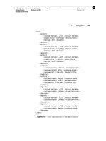
IXQFWLRQ>[\]@ WRUXVUQD

72586*HQHUDWHDWRUXV
WRUXVUQDJHQHUDWHVDSORWRID
WRUXVZLWKFHQWUDOUDGLXVDDQG
ODWHUDOUDGLXVUQFRQWUROVWKH
QXPEHURIIDFHWVRQWKHVXUIDFH
7KHVHLQSXWYDULDEOHVDUHRSWLRQDO
ZLWKGHIDXOWVU Q D 
>[\]@ WRUXVUQDJHQHUDWHV
WKUHHQE\QPDWULFHVVR
WKDWVXUI[\]ZLOOSURGXFHWKH
WRUXV6HHDOVR63+(5(&</,1'(5
LIQDUJLQD HQG
LIQDUJLQQ HQG
LIQDUJLQU HQG
WKHWD SLQQ
SKL SLQQ
[[ DUFRVSKLFRVWKHWD
\\ DUFRVSKLVLQWKHWD
© 2002 by CRC Press LLC
]] UVLQSKLRQHVVL]HWKHWD
LIQDUJRXW 
VXUI[[\\]]
DU DUVTUW
D[LV>DUDUDUDUDUDU@
HOVH
[ [[
\ \\
] ]]
HQG
Other three-dimensional plotting functions you may wish

to explore via
KHOS are PHVK], VXUIF, VXUIO, FRQWRXU,
and
SFRORU.
12. Advanced Graphics
MATLAB possesses a number of other advanced
graphics capabilities. Significant ones are object-based
graphics, called Handle Graphics, and Graphical User
Interface (GUI) tools.
12.1 Handle Graphics
Beyond those just described, MATLAB’s graphics
system provides low-level functions that let you control
virtually all aspects of the graphics environment to
produce sophisticated plots. The commands
VHW and JHW
allow access to all the properties of your plots. Try
VHWJFI to see some of the properties of a figure that
you can control. This system is called Handle Graphics.
See Using MATLAB Graphics for more information.
12.2 Graphical user interface
MATLAB’s graphics system also provides the ability to
add sliders, push-buttons, menus, and other user interface
controls to your own figures. For information on creating
user interface controls, try
KHOS XLFRQWURO. This
© 2002 by CRC Press LLC
allows you to create interactive graphical-based
applications.
Try
JXLGH (short for Graphic User Interface

Development Environment). This brings up MATLAB’s
Layout Editor window that you can use to interactively
design a graphic user interface.
For more information, see the online document Creating
Graphical User Interfaces.
13. Sparse Matrix Computations
A sparse matrix is one with mostly zero entries.
MATLAB provides the capability to take advantage of
the sparsity of matrices.
13.1 Storage modes
MATLAB has two storage modes, full and sparse, with
full the default. The functions
IXOO and VSDUVH convert
between the two modes. Nearly all MATLAB operators
and functions operate seamlessly on both full and sparse
matrices. For a matrix
$, full or sparse, QQ]$ returns
the number of nonzero elements in A.
An
P-by-Q sparse matrix is stored in three one-
dimensional arrays. Numerical values and their row
indices are stored in two arrays of size
QQ]$ each. All
of the entries in any given column are stored
contiguously. A third array of size
Q holds the
positions in the other two arrays of the first nonzero entry
in each column. Thus, if
$ is sparse, then [ $
takes much more time than

[ $, and V $ is
also slow. To get high performance when dealing with
sparse matrices, use matrix expressions instead of
IRU
© 2002 by CRC Press LLC
loops and vector or scalar expressions. If you must
operate on the rows of a sparse matrix
$, try working with
the columns of
$ instead.
If a full tridiagonal matrix
) is created via, say,
) IORRUUDQG
) WULXWULO)
then the statement 6 VSDUVH) will convert ) to sparse
mode. Try it. Note that the output lists the nonzero
entries in column major order along with their row and
column indices because of how sparse matrices are
stored. The statement
) IXOO6 returns ) in full
storage mode. You can check the storage mode of a
matrix
$ with the command LVVSDUVH$.
13.2 Generating sparse matrices
A sparse matrix is usually generated directly rather than
by applying the function
VSDUVH to a full matrix. A
sparse banded matrix can be easily created via the
function
VSGLDJV by specifying diagonals. For example,

a familiar sparse tridiagonal matrix is created by:
P 
Q 
H RQHVQ
G H
7 VSGLDJV>HGH@>@PQ
Try it. The integral vector >@ specifies in which
diagonals the columns of
>HGH@ should be placed (use
IXOO7 to see the full matrix 7 and VS\7 to view 7
graphically). Experiment with other values of
P and Q
and, say,
>@ instead of >@. See KHOS
VSGLDJV for further features of VSGLDJV.
© 2002 by CRC Press LLC
The sparse analogs of H\H, ]HURV, RQHV, and UDQG for
full matrices are, respectively,
VSH\H, VSDUVH, VSRQHV,
and
VSUDQG. The latter two take a matrix argument and
replace only the nonzero entries with ones and uniformly
distributed random numbers, respectively.
VSDUVHPQ
creates a sparse zero matrix.
VSUDQG also permits the
sparsity structure to be randomized. This is a useful
method for generating simple sparse test matrices, but be
careful. Random sparse matrices are not truly "sparse"
because of catastrophic fill-in when they are factorized

(see Section 13.4). Sparse matrices arising in real
applications typically do not share this characteristic.
4

The versatile function
VSDUVH also permits creation of a
sparse matrix via listing its nonzero entries:
L >@
M >@
V >@
6 VSDUVHLMV
IXOO6
The last two arguments to VSDUVH in the example above
are optional. They tell
VSDUVH the dimensions of the
matrix; if not present, then
6 will be PD[L by PD[M.
If there are repeated entries in
>LM@, then the entries are
added together. The commands below create a matrix
whose diagonal entries are
, , and .
L >@
M >@
V >@
6 VSDUVHLMV
IXOO6

4
See for a

wide range of sparse matrices arising in real applications.
© 2002 by CRC Press LLC
The entries in L, M, and V can be in any order (the same
order for all three arrays, of course). In general, if the
vector
V lists the nonzero entries of 6 and the integral
vectors
L and M list their corresponding row and column
indices, then:
VSDUVHLMVPQ
will create the desired sparse P-by-Q matrix 6. As another
example try:
Q 
H IORRUUDQGQ
( VSDUVHQQHQQ
13.3 Computation with sparse matrices
The arithmetic operations and most MATLAB functions
can be applied independent of storage mode. The storage
mode of the result depends on the storage mode of the
operands or input arguments. Operations on full matrices
always give full results. If
) is a full matrix, 6 and V are
sparse, and
Q is a scalar, then these operations give sparse
results:
6666666)
6AQ6AQ6?V
LQY6FKRO6OX6
GLDJ6PD[6VXP6
These give full results:

6))?66)
6)6?))6
unless ) is a scalar, in which case 6), )?6, and 6) are
sparse.
© 2002 by CRC Press LLC
A matrix built from blocks, such as >$%&'@, is
stored in sparse mode if any constituent block is sparse.
To compute the eigenvalues or singular values of a sparse
matrix
6, you must convert 6 to a full matrix and then use
HLJ or VYG, as HLJIXOO6 or VYGIXOO6. If 6
is a large sparse matrix and you wish only to compute
some of the eigenvalues or singular values, then you can
use the
HLJV or VYGV functions (HLJV6 or VYGV6).
13.4 Ordering methods
When MATLAB solves a sparse linear system ([ $?E), it
typically starts by computing the LU, QR, or Cholesky
factorization of
$. This usually leads to fill-in, or the
creation of new nonzeros in the factors that do not appear
in
$. MATLAB provides several methods that attempt to
reduce fill-in by reordering the rows and columns of
$:
FRODPG approximate minimum degree
FROPPG multiple minimum degree
FROSHUP sort columns by number of nonzeros
V\PDPG symmetric approximate min. degree
V\PPPG symmetric multiple minimum degree

V\PUFP reverse Cuthill-McKee
The first three find a column ordering of
$ and are best
used for
OX or TU. The next three are primarily for FKRO
and return an ordering to be applied symmetrically to
both the rows and columns of a symmetric matrix
$ (they
can also be used for unsymmetric matrices). Finding the
best ordering is so difficult that it is practically impossible
for most matrices. Fast non-optimal heuristics are used
instead, which means that no one method is always the
best. MATLAB uses
FROPPG and V\PPPG by default in
© 2002 by CRC Press LLC
[ $?E
, although FRODPG and V\PDPG tend to be faster
and find better orderings.
Create the
WU\BOX function, which also illustrates the use
of permutation vectors, the
VS\, VXESORW, QRUPHVW, and
HWUHHSORW functions, and how to get a close estimate of
the flop count for LU factorization if we assume that all
zeros are taken advantage of:
IXQFWLRQWU\BOX$PHWKRGLVV\P
VSDUVH/8IDFWRUL]DWLRQRI$
ILJXUH
FOIUHVHW
VXESORW

VS\$
WLWOH2ULJLQDOPDWUL[$
W FSXWLPH
LIQDUJLQ!
6 VSRQHV$VSRQHV$
S IHYDOPHWKRG6
$ $SS
HOVHLIQDUJLQ!
T IHYDOPHWKRG$
$ $T
HQG
WRUGHU FSXWLPHW
VXESORW
VS\$
WLWOH3HUPXWHGPDWUL[$
W FSXWLPH
>/83@ OX$
WOX FSXWLPHW
WRWDO WRUGHUWOX
VXESORW
VS\/8
WLWOH/8IDFWRUV
QRUPHVW/83$
/Q] IXOOVXPVSRQHV/
8Q] IXOOVXPVSRQHV8
IORSBFRXQW /Q]8Q]VXP/Q]
VXESORW
© 2002 by CRC Press LLC
6 VSRQHV$
HWUHHSORW66

WLWOHFROXPQHOLPLQDWLRQWUHH
Next, try this, which evaluates the quality of several
ordering methods with a sparse matrix from a chemical
process simulation problem:
ORDGZHVW
$ ZHVW
WU\BOX$
WU\BOX$#FROSHUP
WU\BOX$#V\PUFP
WU\BOX$#FROPPG
WU\BOX$#FRODPG
See how much sparsity helped by trying this (the flop
count will be wrong, though):
WU\BOXIXOO$
13.5 Visualizing matrices
The previous section gave an example of how to use VS\
to plot the nonzero pattern of a sparse matrix.
VS\ can
also be used on full matrices. It is useful for matrix
expressions coming from relational operators. Try this,
for example (see Chapter 7 for the
GGRP function):
$ >



@
& GGRP$
ILJXUH
VS\$a &

VS\$!
© 2002 by CRC Press LLC