neural networks algorithms applications and programming techniques phần 3 docx
Bạn đang xem bản rút gọn của tài liệu. Xem và tải ngay bản đầy đủ của tài liệu tại đây (1011.54 KB, 41 trang )
2.3 Applications of Adaptive Signal Processing
71
Current signal
Prediction of
current signal
Past signal
Figure 2.16 This schematic shows an adaptive filter used to predict signal
values. The input signal used to train the network is a delayed
value of the actual signal; that is, it is the signal at some past
time. The expected output is the current value of the signal.
The adaptive filter attempts to minimize the error between its
output and the current signal, based on an input of the signal
value from some time in the past. Once the filter is correctly
predicting the current signal based on the past signal, the
current signal can be used directly as an input without the
delay. The filter will then make a prediction of the future
signal value.
Input signals
Prediction of
plant output
Figure
2.17
This example shows an adaptive filter used to model the
output from a system, called the plant. Inputs to the filter are
the same as those to the plant. The filter adjusts its weights
based on the difference between its output and the output of
the plant.
L
72
Adaline and
Madaline
magnetic radiation, we broaden the definition here to include any spatial array
of sensors. The basic task here is to learn to steer the array. At any given time,
a signal may be arriving from any given direction, but antennae usually are
directional in their reception characteristics: They respond to signals in some
directions, but not in others. The antenna array with adaptive filters learns to
adjust its directional characteristics in order to respond to the incoming signal
no matter what the direction is, while reducing its response to unwanted noise
signals coming in from other directions.
Of course, we have only touched on the number of applications for these
devices. Unlike many other neural-network architectures, this is a relatively
mature device with a long history of success. In the next section, we replace
the binary output condition on the ALC circuit so that the latter becomes, once
again, the complete Adaline.
2.4 THE MADALINE
As you can see from the discussion in Chapter 1, the Adaline resembles the
perceptron closely; it also has some of the same limitations as the perceptron.
For example, a two-input Adaline cannot compute the XOR function. Com-
bining Adalines in a layered structure can overcome this difficulty, as we did in
Chapter 1 with the perceptron. Such a structure is illustrated in Figure 2.18.
Exercise 2.5: What logic function is being computed by the single Adaline in
the output layer of Figure
2.18?
Construct a three-input Adaline that computes
the majority function.
2.4.1 Madaline Architecture
Madaline is the acronym for Many Adalines. Arranged in a multilayered archi-
tecture as illustrated in Figure 2.19, the Madaline resembles the general neural-
network structure shown in Chapter
1.
In this configuration, the Madaline could
be presented with a large-dimensional input
vector—say,
the pixel values from
a raster scan. With suitable training, the network could be taught to respond
with a binary
+1
on one of several output nodes, each of which corresponds to
a different category of input image. Examples of such categorization are
{cat,
dog, armadillo, javelina} and {Flogger, Tom Cat, Eagle,
Fulcrum}.
In such a
network, each of four nodes in the output layer corresponds to a single class.
For a given input pattern, a node would have a
+1
output if the input pattern
corresponded to the class represented by that particular node. The other three
nodes would have a
-1
output. If the input pattern were not a member of any
known class, the results from the network could be ambiguous.
To train such a network, we might be tempted to begin with the LMS
algorithm at the output layer. Since the network is presumably trained with
previously identified input patterns, the desired output vector is known. What
2.4 The Madaline
73
=
-1.5
Figure 2.18 Many Adalines (the Madaline) can compute the XOR
function of two inputs. Note the addition of the bias terms to
each Adaline. A positive analog output from an ALC results
in a +1 output from the associated Adaline; a negative analog
output results in a
-1.
Likewise, any inputs to the device that
are binary in nature must use ±1 rather than 1 and 0.
we do not know is the desired output for a given node on one of the hidden
layers. Furthermore, the LMS algorithm would operate on the analog outputs
of the ALC, not on the bipolar output values of the Adaline. For these reasons,
a different training strategy has been developed for the Madaline.
2.4.2 The
MRII
Training Algorithm
It is possible to devise a method of training a
Madaline-like
structure based on
the LMS algorithm; however, the method relies on replacing the linear threshold
output function with a continuously differentiable function (the threshold func-
tion is discontinuous at 0; hence, it is not differentiable there). We
will
take up
the study of this method in the next chapter. For now, we consider a method
known as Madaline rule II (MRII). The original Madaline rule was an earlier
74
Adaline and Madaline
Output layer
of
Madalines
Hidden layer
of Madalines
Figure
2.19
Many Adalines can be joined in a layered neural network
such as this one.
method that we shall not discuss here. Details can be found in references given
at the end of this chapter.
MRII
resembles a
trial-and-error
procedure with added intelligence in the
form of a minimum disturbance principle. Since the output of the network
is a series of bipolar units, training amounts to reducing the number of incor-
rect output nodes for each training input pattern. The minimum disturbance
principle enforces the notion that those nodes that can affect the output error
while incurring the least change in their weights should have precedence in the
learning procedure. This principle is embodied in the following algorithm:
1. Apply a training vector to the inputs of the Madaline and propagate it
through to the output units.
2. Count the number of incorrect values in the output layer; call this number
the error.
3. For all units on the output layer,
a. Select the first previously unselected node whose analog output is clos-
est to zero. (This node is the node that can reverse its bipolar output
2.4 The Madaline 75
with the least change in its
weights—hence
the term minimum distur-
bance.)
b. Change the weights on the selected unit such that the bipolar output of
the unit changes.
c. Propagate the input vector forward from the inputs to the outputs once
again.
d. If the weight change results in a reduction in the number of errors,
accept the weight change; otherwise, restore the original
weights
4. Repeat step 3 for all layers except the input layer.
5. For all units on the output layer,
a. Select the previously unselected pair of units whose analog outputs are
closest to zero.
b. Apply a weight correction to both units, in order to change the bipolar
output of each.
c. Propagate the input vector forward from the inputs to the outputs.
d. If the weight change results in a reduction in the number of errors,
accept the weight change; otherwise, restore the original weights.
6. Repeat step 5 for all layers except the input layer.
If necessary, the sequence in steps 5 and 6 can be repeated with triplets
of units, or quadruplets of units, or even larger combinations, until satisfactory
results are obtained. Preliminary indications are that pairs are adequate for
modest-sized networks with up to 25 units per layer
[8].
At the time of this writing, the
MRII
was still undergoing experimentation
to determine its convergence characteristics and other properties. Moreover, a
new learning algorithm,
MRIII,
has been developed.
MRIII
is similar to MRII,
but the individual units have a continuous output function, rather than the bipolar
threshold function
[2].
In the next section, we shall use a Madaline architecture
to examine a specific problem in pattern recognition.
2.4.3 A Madaline for Translation-Invariant
Pattern Recognition
Various Madaline structures have been used recently to demonstrate the appli-
cability of this architecture to adaptive pattern recognition having the properties
of translation invariance, rotation invariance, and scale invariance. These three
properties are essential to any robust system that would be called on to rec-
ognize objects in the field of view of optical or infrared sensors, for example.
Remember, however, that even humans do not always instantly recognize ob-
jects that have been rotated to unfamiliar orientations, or that have been scaled
significantly smaller or larger than their everyday size. The point is that there
may be alternatives to training in instantaneous recognition at all angles and
scale factors. Be that as it may, it is possible to build neural-network devices
that exhibit these characteristics to some degree.
76
Adaline and
Madaline
Figure 2.20 shows a portion of a network that is used to implement transla-
tion-invariant recognition of a pattern
[7].
The retina is a 5-by-5-pixel array on
which bit-mapped representation of patterns, such as the letters of the alphabet,
can be placed. The portion of the network shown is called a slab. Unlike a
layer, a slab does not communicate with other slabs in the network, as will be
seen shortly. Each Adaline in the slab receives the identical 25 inputs from the
retina, and computes a bipolar output in the usual fashion; however, the weights
on the 25 Adalines share a unique relationship.
Consider the weights on the top-left Adaline as being arranged in a square
matrix duplicating the pixel array on the retina. The Adaline to the immediate
Madaline slab
Retina
Figure
2.20
This
single
slab
of
Adalines
will
give
the
same
output
(either
+ 1 or -1) for a particular pattern on the retina, regardless
of the horizontal or vertical alignment of that pattern on
the retina. All 25 individual Adalines are connected to a
single Adaline that computes the majority function: If most
of the inputs are +1, the majority element responds with a
+ 1 output. The network derives its translation-invariance
properties from the particular configuration of the weights.
See the text for details.
2.4 The Madaline
77
right of the top-left pixel has the identical set of weight values, but translated
one pixel to the right: The rightmost column of weights on the first unit wraps
around to the left to become the leftmost column on the second unit. Similarly,
the unit below the top-left unit also has the identical weights, but translated
one pixel down. The bottom row of weights on the first unit becomes the top
row of the unit under it. This translation continues across each row and down
each column in a similar manner. Figure 2.21 illustrates some of these weight
matrices. Because of this relationship among the weight matrices, a single
pattern on the retina will elicit identical responses from the slab, independent
Key weight matrix: top row, left column Weight matrix: top row, 2nd column
w w w w
12 13 14 15
"22
^23
^24
W
25
W
32
^33
^34
^35
^42
W
43
W
44
W
45
W
52
W
53
W
54
W
55
Weight matrix: 2nd row, left column
W W W W
51 52 53 45
5J
W W W W
22 23 24 25
w
12
W
13
W
35
W
22
W
23
W
24
W
32
W
33
W
34
W
45
W
42
W
43
W
52
W
53
W
44
W
32
WWW
33 34 35
W W
42 43
W
W
A
,
44 45
Weight matrix: 5th row, 5th column
~
W
55
W
45
W
35
W
25
W
15
W
54
W
44
W
34
W
24
^14
W
53
W
43
W
33
W
23
W
,3
^52
W
42
W
32
W
22
WK
W
S\
W
41
W
3\
tv
21
^11
Figure 2.21 The weight matrix in the upper left is the key weight matrix.
All other weight matrices on the slab are derived from this
matrix. The matrix to the right of the key weight matrix
represents the matrix on the
Adaline
directly to the right of the
one with the key weight matrix. Notice that the fifth column
of the key weight matrix has wrapped around to become the
first column, with the other columns shifting one space to
the right. The matrix below the key weight matrix is the
one on the Adaline directly below the Adaline with the key
weight matrix. The matrix diagonal to the key weight matrix
represents the matrix on the Adaline at the lower right of the
slab.
78
Adaline and
Madaline
of the pattern's translational position on the retina. We encourage you to reflect
on this result for a moment (perhaps several moments), to convince yourself of
its validity.
The majority node is a single Adaline that computes a binary output based
on the outputs of the majority of the Adalines connecting to it. Because of the
translational relationship among the weight vectors, the placement of a particular
pattern at any location on the retina will result in the identical output from the
majority element (we impose the restriction that patterns that extend beyond
the retina boundaries will wrap around to the opposite side, just as the various
weight matrices are derived from the key weight
matrix.).
Of course, a pattern
different from the first may elicit a different response from the majority element.
Because only two responses are possible, the slab can differentiate two classes on
input patterns. In terms of hyperspace, a slab is capable of dividing
hyperspace
into two regions.
To overcome the limitation of only two possible classes, the retina can be
connected to multiple slabs, each having different key weight matrices (Widrow
and Winter's term for the weight matrix on the top-left element of each slab).
Given the binary nature of the output of each slab, a system of n slabs could
differentiate 2" different pattern classes. Figure 2.22 shows four such slabs
producing a four-dimensional output capable of distinguishing
16
different input-
pattern classes with translational invariance.
Let's review the basic operation of the translation invariance network in
terms of a specific example. Consider the
16
letters A
—>
P, as the input patterns
we would like to identify regardless of their
up-down
or left-right translation
on the 5-by-5-pixel retina. These translated retina patterns are the inputs to the
slabs of the network. Each retina pattern results in an output pattern from the
invariance network that maps to one of the 16 input classes (in this case, each
class represents a letter). By using a lookup table, or other method, we can
associate the 16 possible outputs from the invariance network with one of the
16 possible letters that can be identified by the network.
So far, nothing has been said concerning the values of the weights on the
Adalines of the various slabs in the system. That is because it is not actually
necessary to train those nodes in the usual sense. In fact, each key weight
matrix can be chosen at random, provided that each input-pattern class result in
a unique output vector from the invariance network. Using the example of the
previous paragraph, any translation of one of the letters should result in the same
output from the invariance network. Furthermore, any pattern from a different
class (i.e., a different letter) must result in a different output vector from the
network. This requirement means that, if you pick a random key weight matrix
for a particular slab and find that two letters give the same output pattern, you
can simply pick a different weight matrix.
As an alternative to random selection of key weight matrices, it may be
possible to optimize selection by employing a training procedure based on the
MRII.
Investigations in this area are ongoing at the time of this writing
[7].
2.5 Simulating the Adaline
79
Retina
°4
Figure
2.22
Each
of the
four
slabs
in the
system
depicted
here
will
produce
a +1 or a — 1 output value for every pattern that appears on
the retina. The output vector is a four-digit binary number,
so the system can potentially differentiate up to 16 different
classes of input patterns.
L
2.5 SIMULATING THE ADALINE
As we shall for the implementation of all other network simulators we will
present, we shall begin this section by describing how the general data struc-
tures are used to model the Adaline unit and Madaline network. Once the basic
architecture has been presented, we will describe the algorithmic process needed
to propagate signals through the Adaline. The section concludes with a discus-
sion of the algorithms needed to cause the Adaline to self-adapt according to
the learning laws described previously.
2.5.1 Adaline Data Structures
It is appropriate that the Adaline is the first test of the simulator data structures
we presented in Chapter 1 for two reasons:
1. Since the forward propagation of signals through the single Adaline is vir-
tually identical to the forward propagation process in most of the other
networks we will study, it is beneficial for us to observe the Adaline to
80
Adaline and
Madaline
gain a better understanding of what is happening in each unit of a larger
network.
2. Because the Adaline is not a network, its implementation exercises the
versatility of the network structures we have defined.
As we have already seen, the Adaline is only a single processing unit.
Therefore, some of the generality we built into our network structures will not
be required. Specifically, there will be no real need to handle multiple units and
layers of units for the Adaline. Nevertheless, we will include the use of those
structures, because we would like to be able to extend the Adaline easily into
the Madaline.
We begin by defining our network record as a structure that will contain
all the parameters that will be used globally, as well as pointers to locate the
dynamic arrays that will contain the network data. In the case of the Adaline,
a good candidate structure for this record will take the form
record Adaline =
mu
: float;
input:
"layer;
output :
"layer;
end record
{Storage
for stability
term}
{Pointer
to input
layer}
{Pointer
to output
layer}
Note that, even though there is only one unit in the Adaline, we will use
two
layers
to
model
the
network.
Thus,
the
input
and
output
pointers
will
point
to
different
layer
records.
We do
this
because
we
will
use the
input
layer as storage for holding the input signal vector to the Adaline. There will be
no connections associated with this layer, as the input will be provided by some
other process in the system (e.g., a time-multiplexed
analog-to-digital
converter,
or an array of sensors).
Conversely,
the
output
layer
will
contain
one
weight
array
to
model
the
connections
between
the
input
and the
output
(recall
that
our
data
structures
presume that PEs process input connections primarily). Keeping in mind that
we would like to extend this structure easily to handle the Madaline network,
we will retain the indirection to the connection weight array provided by the
weight_ptr
array described in Chapter
1.
Notice that, in the case of the
Adaline,
however,
the
weight_ptr
array
will
contain
only
one
value,
the
pointer to the input connection array.
There is one other thing to consider that may vary between Adaline units.
As we have seen previously, there are two parts to the Adaline structure: the
linear ALC and the bipolar Adaline units. To distinguish between them, we
define an enumerated type to classify each Adaline neuron:
type NODE_TYPE : {linear,
binary};
We now
have
everything
we
need
to
define
the
layer
record
structure
for
the Adaline. A prototype structure for this record is as follows.
2.5 Simulating the
Adaline
record layer =
activation : NODE_TYPE
{kind
of Adaline
node}
outs:
~float[];
{pointer
to unit output
array}
weights :
""float[];
{indirect
access to weight
arrays}
end record
Finally, three dynamically allocated arrays are needed to contain the output
of the
Adaline
unit,
the
weight_ptrs
and the
connection
weights
values.
We will not specify the structure of these arrays, other than to indicate that the
outs
and
weights
arrays
will
both
contain
floating-point
values,
whereas
the
weight_ptr
array
will
store
memory
addresses
and
must
therefore
contain
memory pointer types. The entire data structure for the Adaline simulator is
depicted in Figure 2.23.
2.5.2 Signal Propagation Through the Adaline
If signals are to be propagated through the Adaline successfully, two activities
must occur: We must obtain the input signal vector to stimulate the Adaline,
and the Adaline must perform its input-summation and output-transformation
functions. Since the origin of the input signal vector is somewhat application
specific, we will presume that the user will provide the code necessary to keep
the
data
located
in the
outs
array
in the
Adaline.
inputs
layer
current.
We shall now concentrate on the matter of computing the input stimulation
value and transforming it to the appropriate output. We can accomplish this
task through the application of two algorithmic functions, which we will name
sunuinputs
and
compute_output.
The
algorithms
for
these
functions
are
as follows:
outputs
weights
Figure 2.23 The Adaline simulator data structure is shown.
82
Adaline and Madaline
function
sum_inputs
(INPUTS
WEIGHTS
return float
var sum
:
float;
temp : float;
ins : "float[];
wts :
'float[];
i
:
integer;
begin
sum = 0;
ins = INPUTS;
wts = WEIGHTS'
float[])
{local
accumulator}
{scratch
memory}
{local
pointer}
{local
pointer}
{iteration
counter}
{initialize
accumulator}
{locate
input
array}
{locate
connection
array}
for i = 1 to length(wts) do
{for
all weights in
array}
temp = ins[i] *
wts[i];
{modulate
input}
sum = sum + temp;
{sum
modulated
inputs}
end do
return(sum);
end function;
{return
the modulated
sum}
function compute_output (INPUT : float;
ACT : NODE TYPE) return float
begin
if (ACT = linear)
then return (INPUT)
else
if (INPUT >= 0.0)
then return
(1.0)
else return (-1.0)
end function;
{if
the Adaline is a linear
unit}
{then
just return the
input}
{otherwise}
{if
the input is
positive}
{then
return a binary
true}
;
{else
return a binary
false}
2.5.3 Adapting the Adaline
Now that our simulator can forward propagate signal information, we turn our at-
tention to the implementation of the learning algorithms. Here again we assume
that the input signal pattern is placed in the appropriate array by an application-
specific process. During training, however, we will need to know what the
target output
d^
is for every input vector, so that we can compute the error term
for the Adaline.
Recall that, during training, the
LMS
algorithm requires that the Adaline
update its weights after every forward propagation for a new input pattern.
We must also consider that the Adaline application may need to adapt the
2.5 Simulating the
Adaline
S3
Adaline while it is running. Based on these observations, there is no need
to store or accumulate errors across all patterns within the training algorithm.
Thus, we can design the training algorithm merely to adapt the weights for a
single pattern. However, this design decision places on the application pro-
gram the responsibility for determining when the Adaline has trained suffi-
ciently.
This approach is usually acceptable because of the advantages it offers over
the implementation of a self-contained training loop. Specifically, it means that
we can use the same training function to adapt the Adaline initially or while
it is on-line. The generality of the algorithm is a particularly useful feature,
in that the application program merely needs to detect a condition requiring
adaptation. It can then sample the input that caused the error and generate the
correct response "on the fly," provided we have some way of knowing that
the error is increasing and can generate the correct desired values to accom-
modate retraining. These values, in turn, can then be input to the Adaline
training algorithm, thus
allowing
adaptation at run time. Finally, it also re-
duces the housekeeping chores that must be performed by the simulator, since
we will not need to maintain a list of expected outputs for all training pat-
terns.
We must now define algorithms to compute the squared error term
(£
2
(t)),
the approximation of the gradient of the error surface, and to update the con-
nection weights to the Adaline. We can again simplify matters by combin-
ing the computation of the error and the update of the connection weights
into one function, as there is no need to compute the former without
performing the latter. We now present the algorithms to accomplish these
functions:
function
compute_error
(A : Adaline; TARGET : float)
return float
var tempi : float;
{scratch
memory}
temp2 : float;
{scratch
memory}
err : float;
{error
term for
unit}
begin
tempi =
sum_inputs
(A.input.outs,
A.output.weights);
temp2 =
compute_output
(tempi,
A.output~.activation)
;
err
=
absolute (TARGET -
temp2);
{fast
error}
return
(err);
{return
error}
end function;
function
update_weights
(A : Adaline; ERR : float)
return void
var grad : float;
{the
gradient of the
error}
ins :
"float[];
{pointer
to inputs
array}
wts :
"float[];
{pointer
to weights
array}
i : integer;
{iteration
counter}
84
Adaline and
Madaline
begin
ins =
A.input.outs;
{locate
start of input
vector}
= A. output.weights";
{locate
start of
connections)
for i = 1 to
length(wts)
do
{for
all connections,
do}
grad = -2 * err *
ins[i];
{approximate
gradient}
wts[i]
=
wts[i]
- grad *
A.mu;
{update
connection}
end
do;
end function;
2.5.4 Completing the Adaline Simulator
The algorithms we have just defined are sufficient to implement an Adaline
simulator in both learning and operational modes. To offer a clean interface
to any external program that must call our simulator to perform an Adaline
function, we can combine the modules we have described into two higher-level
functions. These functions will perform the two types of activities the Adaline
must
perform:
f
orwarcLpropagate
and
adapt-Adaline.
function
forward_jaropagate
var tempi : float;
(A : Adaline) return void
{scratch
memory}
begin
tempi =
sum_inputs
(A.inputs.outs,
A. outputs.weights);
A.outputs.outs[1]
=
compute_output
A.node_type);
end function;
(tempi.
function adapt_Adaline
return float
var err : float;
(A : Adaline; TARGET : float)
{train
until
small}
begin
forward_propagate
(A);
{Apply
input
signal}
err =
compute_error
(A,
TARGET);
{Compute
error}
update_weights
(A,
err);
{Adapt
Adaline}
return(err);
end function;
2.5.5 Madaline Simulator Implementation
As we have discussed earlier, the Madaline network is simply a collection of
binary Adaline units, connected together in a layered structure. However, even
though they share the same type of processing unit, the learning strategies
imple-
2.5 Simulating the Adaline
85
mented for the Madaline are significantly different, as described in Section 2.5.2.
Providing that as a guide, along with the discussion of the data structures needed,
we leave the algorithm development for the Madaline network to you as an ex-
ercise.
In this regard, you should note that the layered structure of the Madaline
lends itself directly to our simulator data structures. As illustrated in Figure 2.24,
we can implement a layer of Adaline units as easily as we created a single
Adaline.
The
major
differences
here
will
be the
length
of the
cuts
arrays
in
the
layer
records
(since
there
will
be
more
than
one
Adaline
output
per
layer),
and the
length
and
number
of
connection
arrays
(there
will
be one
weights
array
for
each
Adaline
in the
layer,
and the
weight.ptr
array
will
be
extended
by one
slot
for
each
new
weights
array).
Similarly,
there
will
be
more
layer
records
as the
depth
of the
Madaline
increases, and, for each layer, there will be a corresponding increase in the
number
of
cuts,
weights,
and
weight.ptr
arrays.
Based
on
these
ob-
servations, one fact that becomes immediately perceptible is the combinatorial
growth of both memory consumed and computer time required to support a lin-
ear growth in network size. This relationship between computer resources and
model sizing is true not only for the Madaline, but for all ANS models we will
study. It is for these reasons that we have stressed optimization in data structures.
outputs
Madaline
activation
outs
weights
/
We
——————
^-
°3
ight p
"X
A
W^
A
w
3
^•^^
outputs
weights
Figure 2.24 Madaline data structures are shown.
86
Adaline and
Madaline
Programming Exercises
2.1. Extend the Adaline simulator to include the bias unit, 0, as described in the
text.
2.2. Extend the simulator to implement a three-layer Madaline using the algo-
rithms discussed in Section 2.3.2. Be sure to use the binary Adaline type.
Test the operation of your simulator by training it to solve the XOR problem
described in the text.
2.3. We have indicated that the network stability term,
it,
can greatly affect the
ability of the Adaline to converge on a solution. Using four different values
for
/z
of your own choosing, train an Adaline to eliminate noise from an
input sinusoid ranging from 0 to
2-n
(one way to do this is to use a scaled
random-number generator to provide the noise). Graph the curve of training
iterations versus
/z.
Suggested Readings
The authoritative text by Widrow and Stearns is the standard reference to the
material contained in this chapter
[9].
The original delta-rule derivation is
contained in a 1960 paper by Widrow and Hoff [6], which is also reprinted in
the collection edited by Anderson and Rosenfeld
[1].
Bibliography
[1]
James A. Anderson and Edward Rosenfeld, editors.
Neurocomputing:
Foun-
dations of Research. MIT Press, Cambridge, MA, 1988.
[2] David Andes, Bernard Widrow, Michael
Lehr,
and Eric Wan.
MRIII:
A
robust algorithm for training analog neural networks. In Proceedings of
the International Joint Conference on Neural Networks, pages I-533-I-
536, January 1990.
[3] Richard W. Hamming. Digital Filters. Prentice-Hall, Englewood Cliffs,
NJ,
1983.
[4] Wilfred Kaplan. Advanced Calculus, 3rd edition. Addison-Wesley, Reading,
MA,
1984.
[5] Alan V. Oppenheim arid Ronald W. Schafer.
Digital
Signal Processing.
Prentice-Hall, Englewood Cliffs, NJ, 1975.
[6] Bernard Widrow and Marcian E. Hoff. Adaptive switching circuits. In 7960
IRE
WESCON
Convention
Record,
New
York,
pages
96-104,
1960. IRE.
[7] Bernard Widrow and Rodney Winter. Neural nets for adaptive filtering and
adaptive pattern recognition. Computer,
21(3):25-39,
March 1988.
Bibliography
87
[8]
Rodney
Winter and Bernard Widrow. MADALINE RULE II: A training
algorithm for neural networks. In Proceedings of the IEEE Second In-
ternational Conference on
Neural
Networks, San Diego, CA,
1:401-408,
July 1988.
[9] Bernard Widrow and Samuel D. Stearns. Adaptive Signal Processing. Signal
Processing Series. Prentice-Hall, Englewood Cliffs, NJ, 1985.
H
R
Backpropagation
There are many potential computer applications that are difficult to implement
because there are many problems unsuited to solution by a sequential process.
Applications that must perform some complex data translation, yet have no
predefined mapping function to describe the translation process, or those that
must provide a "best guess" as output when presented with noisy input data are
but two examples of problems of this type.
An ANS that we have found to be useful in addressing problems requiring
recognition of complex patterns and performing
nontrivial
mapping functions is
the backpropagation network (BPN), formalized first by Werbos [11], and later
by Parker [8] and by
Rummelhart
and McClelland
[7].
This network, illustrated
genetically
in Figure 3.1, is designed to operate as a multilayer, feedforward
network, using the supervised mode of learning.
The chapter begins with a discussion of an example of a problem mapping
character image to ASCII, which appears simple, but can quickly overwhelm
traditional approaches. Then, we look at how the backpropagation network op-
erates to solve such a problem. Following that discussion is a detailed derivation
of the equations that govern the learning process in the backpropagation network.
From there, we describe some practical applications of the BPN as described in
the literature. The chapter concludes with details of the BPN software simulator
within the context of the general design given in Chapter
1.
3.1 THE BACKPROPAGATION NETWORK
To illustrate some problems that often arise when we are attempting to automate
complex pattern-recognition applications, let us consider the design of a com-
puter program that must translate a 5 x 7 matrix of binary numbers representing
the bit-mapped pixel image of an alphanumeric character to its equivalent eight-
bit ASCII code. This basic problem, pictured in Figure 3.2, appears to be
relatively trivial at first glance. Since there is no obvious mathematical function
89
90
Backpropagation
Output read in parallel
Always 1
Always 1
Input applied in parallel
Figure 3.1 The general backpropagation network architecture is shown.
that will perform the desired translation, and because it would undoubtedly take
too much time (both human and computer time) to perform a
pixel-by-pixel
correlation, the best algorithmic solution would be to use a lookup table.
The lookup table needed to solve this problem would be a one-dimensional
linear array of ordered pairs, each taking the form:
record
AELEMENT
=
pattern : long integer;
ascii : byte;
end record;
= 0010010101000111111100011000110001
= 0951FC631
16
=
65
10
ASCII
Figure 3.2 Each character image is mapped to its corresponding ASCII
code.
3.1 The Backpropagation Network
91
The first is the numeric equivalent of the bit-pattern code, which we generate
by moving the seven rows of the matrix to a single row and considering the
result to be a 35-bit binary number. The second is the ASCII code associated
with the character. The array would contain exactly the same number of ordered-
pairs as there were characters to convert. The algorithm needed to perform the
conversion process would take the following form:
function
TRANSLATE(INPUT
: long integer;
LUT
:
"AELEMENT[]>
return ascii;
{performs
pixel-matrix to ASCII character
conversion}
var TABLE :
"AELEMENT[];
found :
boolean;
i : integer;
begin
TABLE = LUT;
{locate
translation
table}
found = false;
{translation
not found
yet}
for i = 1 to
length(TABLE)
do
{for
all items in
table)
if
TABLE[i].pattern
= INPUT
then Found = True; Exit;
{translation
found, quit
loop}
end;
If Found
Then return
TABLE[i].ascii
{return
ascii}
Else return 0
end;
Although the lookup-table approach is reasonably fast and easy to maintain,
there are many situations that occur in real systems that cannot be handled by
this method. For example, consider the same
pixel-image-to-ASCII
conversion
process in a more realistic environment. Let's suppose that our character image
scanner alters a random pixel in the input image matrix due to noise when the
image was read. This single pixel error would cause the lookup algorithm to
return either a null or the wrong ASCII code, since the match between the input
pattern and the target pattern must be exact.
Now consider the amount of additional software (and, hence, CPU time)
that must be added to the lookup-table algorithm to improve the ability of the
computer to "guess" at which character the noisy image should have been.
Single-bit errors are fairly easy to find and correct. Multibit errors become
increasingly difficult as the number of bit errors grows. To complicate matters
even further, how could our software compensate for noise on the image if that
noise happened to make an "O" look like a "Q", or an "E" look like an "F"? If
our character-conversion system had to produce an accurate output all the time,
92
Backpropagation
an inordinate amount of CPU time would be spent eliminating noise from the
input pattern prior to attempting to translate it to ASCII.
One solution to this dilemma is to take advantage of the parallel nature of
neural networks to reduce the time required by a sequential processor to perform
the mapping. In addition, system-development time can be reduced because the
network can learn the proper algorithm without having someone deduce that
algorithm in advance.
3.1.1
The Backpropagation Approach
Problems such as the noisy
image-to-ASCII
example are difficult to solve by
computer due to the basic incompatibility between the machine and the problem.
Most of today's computer systems have been designed to perform mathemati-
cal and logic functions at speeds that are incomprehensible to humans. Even
the relatively unsophisticated desktop microcomputers commonplace today can
perform hundreds of thousands of numeric comparisons or combinations every
second.
However, as our previous example illustrated, mathematical prowess is not
what is needed to recognize complex patterns in noisy environments. In fact,
an algorithmic search of even a relatively small input space can prove to be
time-consuming. The problem is the sequential nature of the computer itself;
the
"fetch-execute"
cycle of the von Neumann architecture allows the machine
to perform only one operation at a time. In most cases, the time required
by the computer to perform each instruction is so short (typically about one-
millionth of a second) that the aggregate time required for even a large program
is insignificant to the human users. However, for applications that must search
through a large input space, or attempt to correlate all possible permutations of
a complex pattern, the time required by even a very fast machine can quickly
become intolerable.
What we need is a new processing system that can examine all the pixels in
the image in parallel. Ideally, such a system would not have to be programmed
explicitly; rather, it would adapt itself to "learn" the relationship between a set of
example patterns, and would be able to apply the same relationship to new input
patterns. This system would be able to focus on the features of an arbitrary input
that resemble other patterns seen previously, such as those pixels in the noisy
image that "look" like a known character, and to ignore the noise. Fortunately,
such a system exists; we call this system the backpropagation network (BPN).
3.1.2 BPN Operation
In Section 3.2, we will cover the details of the mechanics of backpropagation.
A summary description of the network operation is appropriate here, to illustrate
how the BPN can be used to solve complex pattern-matching problems. To begin
with, the network learns a predefined set of
input-output
example pairs by using
a two-phase
propagate-adapt
cycle. After an input pattern has been applied as
a stimulus to the first layer of network units, it is propagated through each upper
3.2 The
Generalized
Delta Rule 93
layer until an output is generated. This output pattern is then compared to the
desired output, and an error signal is computed for each output unit.
The error signals are then transmitted backward from the output layer to
each node in the intermediate layer that contributes directly to the output. How-
ever, each unit in the intermediate layer receives only a portion of the total error
signal, based roughly on the relative contribution the unit made to the original
output. This process repeats, layer by layer, until each node in the network has
received an error signal that describes its relative contribution to the total error.
Based on the error signal received, connection weights are then updated by each
unit to cause the network to converge toward a state that allows all the training
patterns to be encoded.
The significance of this process is that, as the network trains, the nodes
in the intermediate layers organize themselves such that different nodes learn
to recognize different features of the total input space. After training, when
presented with an arbitrary input pattern that is noisy or incomplete, the units in
the hidden layers of the network will respond with an active output if the new
input contains a pattern that resembles the feature the individual units learned
to recognize during training. Conversely, hidden-layer units have a tendency to
inhibit their outputs if the input pattern does not contain the feature that they
were trained to recognize.
As the signals propagate through the different layers in the network, the
activity pattern present at each upper layer can be thought of as a pattern with
features that can be recognized by units in the subsequent layer. The output
pattern generated can be thought of as a feature map that provides an indication
of the presence or absence of many different feature combinations at the input.
The total effect of this behavior is that the BPN provides an effective means of
allowing a computer system to examine data patterns that may be incomplete
or noisy, and to recognize subtle patterns from the partial input.
Several researchers have shown that during training, BPNs tend to develop
internal relationships between nodes so as to organize the training data into
classes of patterns
[5].
This tendency can be extrapolated to the hypothesis
that all hidden-layer units in the BPN are somehow associated with specific
features of the input pattern as a result of training. Exactly what the association
is may or may not be evident to the human observer. What is important is that
the network has found an internal representation that enables it to generate the
desired outputs when given the training inputs. This same internal representation
can be applied to inputs that were not used during training. The BPN will
classify these previously unseen inputs according to the features they share with
the training examples.
3.2 THE GENERALIZED DELTA RULE
In this section, we present the formal mathematical description of BPN op-
eration. We shall present a detailed derivation of the generalized delta
rule
(GDR), which is the learning algorithm for the network.
94
Backpropagation
Figure 3.3 serves as the reference for most of the discussion. The BPN is a
layered, feedforward network that is fully interconnected by layers. Thus, there
are no feedback connections and no connections that bypass one layer to go
directly to a later layer. Although only three layers are used in the discussion,
more than one hidden layer is permissible.
A neural network is called a mapping network if it is able to compute
some functional relationship between its input and its output. For example, if
the input to a network is the value of an angle, and the output is the cosine of
that angle, the network performs the mapping 9
—>
cos(#).
For such a simple
function, we do not need a neural network; however, we might want to perform
a complicated mapping where we do not know how to describe the functional
relationship in advance, but we do know of examples of the correct mapping.
'PN
Figure 3.3
The three-layer BPN architecture follows closely the general
network description given in Chapter
1.
The bias weights,
0^
,
and
Q°
k
,
and the bias units are optional. The bias units provide
a fictitious input value of 1 on a connection to the bias weight.
We can then treat the bias weight (or simply, bias) like any
other weight: It contributes to the net-input
value
to the unit,
and it participates in the learning process like any other weight.
3.2 The Generalized Delta Rule
95
In this situation, the power of a neural network to discover its own algorithms
is extremely useful.
Suppose
we
have
a set of P
vector-pairs,
(xi,yj),
(x
2
,y2), >
(xp,yp),
which are examples of a functional mapping y =
0(x)
: x
€
R^y
6
R
M
-
We want to train the network so that it will learn an approximation o
=
y'
=
</>'(x).
We
shall
derive
a
method
of
doing
this
training
that
usually
works,
provided the training-vector pairs have been chosen properly and there is a suf-
ficient number of them. (Definitions of properly and sufficient will be given
in Section 3.3.) Remember that learning in a neural network means finding an
appropriate set of weights. The learning technique that we describe here re-
sembles the problem of finding the equation of a line that best fits a num-
ber of known points. Moreover, it is a generalization of the LMS rule that
we discussed in Chapter 2. For a line-fitting problem, we would probably
use a least-squares approximation. Because the relationship we are trying to
map is likely to be nonlinear, as well as multidimensional, we employ an it-
erative version of the simple least-squares method, called a steepest-descent
technique.
To begin, let's review the equations for information processing in the three-
layer network in Figure 3.3. An input vector,
x
p
=
(x
p
\,x
p
2, ,x
p
N)
t
,
is
applied to the input layer of the network. The input units distribute the values
to the hidden-layer units. The net input to the
jth
hidden unit is
(3.1)
where
wf
t
is the weight on the connection from the
ith
input unit, and
6^
is
the bias term discussed in Chapter 2. The
"h"
superscript refers to quantities
on the hidden layer. Assume that the activation of this node is equal to the net
input; then, the output of this node is
)
(3.2)
The equations for the output nodes are
L
°
kj
i
pj
+
8°
k
(3.3)
o
pk
=
/>e&)
(3.4)
where the "o" superscript refers to quantities on the output layer.
The initial set of weight values represents a first guess as to the proper
weights for the problem. Unlike some methods, the technique we employ here
does not depend on making a good first guess. There are guidelines for selecting
the initial weights, however, and we shall discuss them in Section 3.3. The basic
procedure for training the network is embodied in the following description: