neural networks algorithms applications and programming techniques phần 6 potx
Bạn đang xem bản rút gọn của tài liệu. Xem và tải ngay bản đầy đủ của tài liệu tại đây (1.22 MB, 41 trang )
194
Simulated Annealing
Co-occurence
A-B
A-C
A-D
A-E
B-C
B-D
B-E
C-D
C-E
D-E
Low memory
High memory
(a)
(b)
Figure 5.5 The
CO-OCCURRENCE
array is shown (a) depicted as a
sequential memory array, and (b) with its mapping to the
connections in the Boltzmann network.
Figure 5.5(a). The first four entries in the CO-OCCURRENCE array for this
network would be mapped to the connections between units A-B, A-C,
A-
D, and A-E, as shown in Figure
5.5(b).
Likewise, the next three slots would
be mapped to the connections between units B-C, B-D, and B-E; the next
two to C-D, and C- E; and the last one to D-E. By using the arrays in this
manner, we can collect co-occurrence statistics about the network by starting
at the first input unit and sequentially scanning all other units in the network.
After completing this initial pass, we can complete the network scan by merely
incrementing our array pointer to access the second unit, then the third, fourth,
,
nth units.
We can now specify the remaining data structures needed to implement
the Boltzmann network simulator. We begin by defining the top-level record
structure used to define the Boltzmann network:
record BOLTZMANN =
UNITS :
integer;
CLAMPED : boolean;
INPUTS : DEDICATED;
OUTPUTS : DEDICATED;
NODES
:
"layer;
TEMPERATURE : float;
CURRENT : integer;
{number
of units in
network}
{true=clamped;
false=unclamped}
{locate
and size network
input}
(locate and size network
output}
{pointer
to layer
structure)
{current
network
temperature}
{step
in annealing
schedule)
5.3 The Boltzmann Simulator
195
ANNEALING :
~SCHEDULE[];
{pointer
to user-defined
schedule}
STATISTICS :
COOCCURRENCE;
{pointers
to statistics
arrays}
end record;
Figure 5.6 provides an illustration of how the values in the BOLTZMANN
structure interact to specify a Boltzmann network. Here, as in other network
models,
the
layer
structure
is the
gateway
to the
network
specific
data
struc-
tures. All that is needed to gain access to the layer-specific data are point-
ers to the
appropriate
arrays.
Thus,
the
structure
for the
layer
record
is
given by
cuts
weights 1
Boltzmann
Nodes
Annealing
Current
.
Figure 5.6 Organization of the Boltzmann network using the defined data
structure is shown. In this example, the input and output
units are the same, and the network is in the third step of
its annealing schedule.
196 Simulated Annealing
record LAYER =
outs
:
~float[];
{pointer
to unit outputs
array}
weights :
~"float[];
{pointers
in weight
_ptr
array}
end record;
where out s is a pointer used to locate the beginning of the unit outputs array
in
memory,
and
weights
is a
pointer
to the
intermediate
weight-ptr
ar-
ray, which is used in turn to locate each of the input connection arrays in the
system. Since the Boltzmann network requires only one layer of PEs, we will
need
only
one
layer
pointer
in the
BOLTZMANN
record.
All
these
low-level
data structures are exactly the same as those specified in the generic simulator
discussed in Chapter
1.
5.3.3 Boltzmann Algorithms
Let us assume, for now, that our network data structures contain valid weights
for all the connections, and that the user has initialized the annealing schedule
to contain the information given in Table
5.1;
in other words, the network data
structures represent a trained network. We must now create the programs that
the host computer will execute to simulate the network in production mode. We
shall start by developing the information-recall routines.
Boltzmann Production Algorithms. Remember that information recall in the
Boltzmann network consists of a sequence of steps where we first apply an
input to the network, raise the temperature to some predefined level, and anneal
the network while slowly lowering the temperature. In this example, we would
initially raise the temperature to 5 and would perform four stochastic signal
propagations; we would then lower the temperature to 4 and would perform
six signal propagations, and so on. After completing the four required signal
propagations when the temperature of the network is 1, we can consider the
network annealed. At this point, we simply read the output values from the
visible units.
If, however, we think about the process we just described, we can decom-
pose the information-recall problem into three lower-level subroutines:
Temperature
5
4
3
2
1
Passes
4
6
7
6
4
Table 5.1 The annealing schedule for the simulator example.
L
5.3 The Boltzmann Simulator 197
apply_input
A
routine
used
to
take
a
user-provided
or
training
input
and
apply it to the network, and to initialize the output from all unknown units
to a random
state,
anneal
A
routine
used
to
stimulate
the
Boltzmann
network
according
to the
previously initialized annealing
schedule,
get-output
A
function
used
to
locate
the
start
of the
output
array
in the
computer memory, so that the network response can be accessed.
Since
the
anneal
routine
is the
place
where
most
of the
processing
is
accomplished, we shall concentrate on the development of just that routine,
leaving the design of the other two algorithms to you. The mathematics of
the Boltzmann network tells us that the annealing process, in production mode,
consists of two major functions that are repeated until the network has stabilized
at a low temperature. These functions, described next, can each be implemented
as
subroutines
that
are
called
by the
parent
anneal
process.
set_temp
A procedure used to set the current network temperature and an-
nealing schedule pass count to values specified in the overall annealing
schedule.
propagate
A
function
used
to
perform
one
signal
propagation
through
the
entire
network,
using
the
current
temperature
and
probabilistic
unit
se-
lection. This routine should be capable of performing the signal propagation
regardless of the network state (clamped or undamped).
Signal Propagation in the Boltzmann Network. We shall now define the
most
basic
of the
needed
subroutines,
the
propagate
procedure.
The al-
gorithm for this procedure, which follows, presumes that the user-provided
apply-input
and
not-yet-defined
set-temp
functions
have
been
executed
to
initialize
the
outputs
of the
network's
units
and
temperature
parameter
to the desired states.
procedure propagate
(NET:BOLTZMANN)
{perform
one signal propagation pass through
network.}
var unit : integer;
{randomly
selected
unit}
p : float;
{probability
of unit being
on}
neti
: float;
{net
input to
unit}
threshold : integer;
{point
at which unit turns
on}
i, j : integer;
{iteration
counters}
inputs :
"float[];
{pointer
to unit outputs
array}
connects :
~float[];
{pointer
to unit weights
array}
undamped : integer;
{index
to first undamped
unit}
firstc : integer;
(index
to first
connection}
begin
{locate
the first nonvisible unit, assuming first
index =
1}
undamped = NET
.OUTPUT.
FIRST + NET . OUTPUT . LENGTH - 1;
198 Simulated Annealing
if
(NET.INPUTS.FIRST
=
NET.OUTPUTS.FIRST)
then firstc =
NET.INPUTS.FIRST
{Boltzmann
completion}
else firstc =
NET.INPUTS.LENGTH
+ 1;
{Boltzmann
input-output}
end
if;
for i = 1 to
NET.UNITS
{for
as many units in
network}
do
if
(NET.CLAMPED)
{if
network is
clamped}
then
{select
an undamped
unit}
unit = random (NET. UNITS - undamped)
+ undamped;
else
{select
any
unit}
unit =
random(NET.UNITS);
end if;
neti
=0;
{initialize
input}
inputs =
NET.NODES".CUTS;
{locate
inputs}
connects =
NET.NODES".WEIGHTS[i]';
{and
connections}
for j = firstc to
NET.UNITS
{all
connections to
unit}
do
{compute
sum of
products}
neti = neti +
inputs[j]
*
connects[j];
end do;
{this
next statement is used to improve
performance, as described in the
text}
if
(NET.INPUTS.FIRST
=
NET.OUTPUTS.FIRST)
or (i >= firstc)
then
neti = neti -
inputs[i]
*
connects[i];
{no
connection}
end if;
p = 1.0 /
(1.0+
exp(-neti
/
NET.TEMPERATURE));
threshold = round (p *
10000);
{convert
to
integer}
if
(random(lOOOO)
<=
threshold))
{should
unit be
on?}
then
inputs[unit]
=1;
{if
so, set to 1}
else
inputs[unit]
= 0;
{otherwise,
set to 0}
end if;
end do;
end procedure;
5.3 The Boltzmann Simulator 199
Before we move on to the next routine, there are three aspects of the
propagate
procedure
that
bear
further
discussion:
the
selection
mechanism
for
unit
update,
the
computation
of the
neti
term,
and the
method
we
have
chosen for determining when a unit is or is not active.
In the first case, the Boltzmann network must be able to run with its in-
puts either clamped or free-running. So that we do not need to have different
propagate
routines
for
each
mode,
we
simply
use a
Boolean
variable
in
the network record to indicate the current mode of operation, and enable the
propagate
routine
to
select
a
unit
for
update
accordingly.
If the
network
is clamped, we cannot select an input or output unit for update. We account
for these differences by assuming that the visible units to the network are the
first
TV
units in the layer. We thus can be assured that the visible units will
not change if we simply select a random unit from the set of units that do not
include the first N units. We accomplish this selection by decreasing the range
of the random-number generator to the number of network units minus N, and
then adding
TV
to the result. Since we have decided that all our arrays will use
the first
TV
indices to locate the visible units, generating a random index greater
than
TV
will always select a random unit beyond the range of the visible units.
However, if the network is undamped, any unit must be available for update.
Inspection
of the
algorithm
for
propagate
will
reveal
that
these
two
cases
are
handled
by the
if-then-else
clause
at the
beginning
of the
routine.
Second,
there
are two
salient points
regarding
the
computation
of the
neti
term
with
respect
to the
propagate
routine.
The
first
point
is
that
connec-
tions between input units are processed only when the network is configured
as a Boltzmann completion network. In the Boltzmann
input-output
mode,
connections between input units do not exist. This structure conforms to the
mathematical model described earlier. The second point about the calculation
of the
neti
term
is
that
we
have
obviously
wasted
computer
time
by
process-
ing a connection from each unit to itself twice, once as part of the summation
loop
during
the
calculation
of the
neti
value,
and
once
to
subtract
it out
after
the
total
neti
has
been
calculated.
The
reason
we
have
chosen
to
implement
the algorithm in this manner is, again, to improve performance. Even though
we have consumed computer time by processing a nonexistent connection for
every unit in the network, we have used far less time than would be required
to disallow the computation of the missing connection selectively during every
iteration of the summation loop. Furthermore, we can easily eliminate the error
introduced in the input summation by processing the nonexistent connection by
subtracting out just that term after completing the loop, prior to updating the
output of the unit. You might also observe that we have wasted memory by
allocating space for the connections between each unit and itself. We have cho-
sen to implement the network in this fashion to simplify processing, and thus
to improve performance as described.
As an example of why it is desirable to optimize the code at the expense
of wasted memory, consider the alternative case where only valid connections
200
Simulated Annealing
are modeled. Since no unit has a connection to itself, but all units have outputs
maintained in the same array, the code to process all input connections to a unit
would have to be written as two different loops: one for those input PEs that
precede the current unit, where the array indices for outputs and connections
correspond one-to-one, and one loop for inputs from units that follow, where
unit outputs are displaced by one array entry from the corresponding connection.
This situation occurs because we have organized the unit outputs and connec-
tions as linearly sequential arrays in memory. Such a situation is illustrated in
Figure 5.7.
(a)
outputs
weights (input)
w
(i-l)j
outputs x weights (input)
(b)
w
(i+2)j
Figure 5.7 The illustration shows array processing (a) when memory is
allocated for all possible connections, and (b) when memory
is not allocated for intra-unit connections. In (a), the code
necessary to perform this input summation simply computes
the input value for all
connections,
then eliminates the error
introduced by processing the nonexistent connection to itself.
In (b), the code must be more selective about accessing
connections, since the one-to-one mapping of connections to
units is lost. Obviously, approach (a) is our preferred method,
since
it
will
execute
much
faster
than
approach
(b).
5.3 The Boltzmann Simulator
201
Finally, with respect to deciding when to activate the output of a unit, recall
that the Boltzmann network differs from the other networks that we have studied
in that PEs are activated stochastically rather than
deterministically.
Recall that
the equation
defines how we calculate the probability that a unit
x/t
is active with respect
to its input stimulation
(net,t).
However, simply knowing the probability that
a unit will generate an output does not guarantee that the unit will generate an
output. We must therefore implement a mechanism that allows the computer to
translate the calculated probability into a unit output that occurs with the same
probability; in effect, we must let the computer roll the dice to determine when
an output is active and when it is not.
One method for doing this is to make use of the pseudorandom-number gen-
erator available in most high-level computer languages. Here, we take advantage
of the fact that the computed probability,
p^,
will always be a fractional number
ranging between zero and one, as illustrated by the graph depicted in Figure 5.8.
We can map
p/,
to an integer threshold value between zero and some arbitrarily
large number by simply multiplying the ceiling value by the computed probabil-
ity and rounding the result into an integer. We then generate a random number
between zero and the selected ceiling, and, if the probability does not exceed
the threshold value just computed, the output of the unit is set to one. Assuming
that the pseudorandom-number generator has a uniform probability distribution
across the interval of interest, the random number produced
will
not exceed the
threshold value with a probability equal to the specified value, pk. Thus, we
now have a means of stochastically activating unit outputs in the network.
-20
-15
-10
0
Net input
Figure 5.8 Shown here is a graph of the probability,
p
k
,
that the
/cth
unit
is on at five different temperatures, T.
202 Simulated Annealing
Boltzmann Learning Algorithms. There are five additional functions that
must be defined to train the Boltzmann network:
set_temp
A
function
used
to
update
the
parameters
in the
BOLTZMANN
record
to reflect the network temperature at the current step, as specified in the
annealing schedule.
pplus
A
function
used
to
compute
and
average
the
co-occurrence
probabilities
for a network with clamped inputs after it has reached equilibrium at the
minimum temperature.
pminus
A
function
similar
to
pplus,
but
used
when
the
network
is
free-
running.
update_connections
The
procedure
that
modifies
the
connection
weights
in the network to train the Boltzmann simulator.
The
implementation
of the
set-temp
function
is
straightforward,
as de-
fined here:
procedure
set_temp
(NET:BOLTZMANN;
N:integer)
{set
the temperature and schedule
step}
begin
NET.CURRENT
= N;
{set
current
step}
NET.TEMPERATURE
=
NET.ANNEALING".STEP[N].TEMPERATURE;
end procedure;
On the other hand, the estimation of the
pj
and
p~
terms is complex,
and each must be accomplished in two steps: in the first, statistics about the
co-occurrence between network units must be gathered and averaged for each
training pattern; in the second, the statistics across all training patterns are
collected. This separation provides a natural breakpoint for algorithm devel-
opment. We can therefore define two algorithms,
sum_cooccurrence
and
pplus,
that
respectively
address
the two
steps
identified.
We shall now turn our attention to the computation of the co-occurrence
probability,
pj,
when the input to the network is clamped to an arbitrary input
vector,
V
a
.
As we did
with
propagate,
we
will
assume
that
the
input
pattern
has
been
placed
on the
input
units
by an
earlier
call
to
set-inputs.
Fur-
thermore, we shall assume that the statistics arrays have been initialized by an
earlier
call
to a
user-supplied
routine
that
we
refer
to as
zero-Statistics.
procedure
sum_cooccurrence
(NET:BOLTZMANN)
{accumulate
co-occurence statistics for the
specified
network}
var i,j,k : integer;
{loop
counters}
connect : integer;
{co-occurence
index}
stats :
"float[];
{pointer
to statistics
array}
5.3 The Boltzmann Simulator 203
begin
if
(NET.CLAMPED)
{if
network is
clamped}
then stats =
NET.STATISTICS.CLAMPED
else stats =
NET.STATISTICS.UNCLAMPED;
end if;
for i = 1 to 5
{arbitrary
number of
cycles}
do
propagate
(NET);
{run
the network
once}
connect = 1;
{start
at first
pair}
for j = 1 to NET.UNITS
{for
all units in
network}
do
if
(NET.NODES.OUTS"[j]
= 1)
{if
unit is
on}
then
for k = j to
NET.UNITS
{for
rest of
units}
do
if (NET.NODES.OUTS~[k] = 1)
then
stats"[connect]
=
stats"[connect]
+ 1;
end
if;
connect = next
(connect);
end do;
else
{skip
to next unit
connect}
connect = connect +
(NET.UNITS
-
j);
end
if;
end do;
end
do;
end procedure;
Notice that the
sum_cooccurrence
routine does not average the accu-
mulated results after completing the examination. We delay this computation
to the
pplus
routine
so
that
we can
continue
to use the
clamped
array
to
collect statistics across all patterns. If we averaged the results after each cycle,
we would be forced to maintain different arrays for each pattern, thus increasing
the need for storage at a near-exponential rate. In addition, note that, by using
a pointer to the appropriate statistics array, we have generalized the routine so
that it may be used to collect statistics for the network in either the clamped or
undamped modes of operation.
Before we define the algorithm needed to estimate the
pt.
term for the
Boltzmann network, we will make a few assumptions. Since the total number of
training patterns that the network must learn will depend on the application, we
204
Simulated Annealing
must write the code so that the computer will calculate the co-occurrence statis-
tics for a variable number of training patterns. We must therefore assume that
the training data are available to the simulator from some external source (such
as a global array or disk file) that we will refer to as PATTERNS, and that the
total number of training patterns contained in this source is obtainable through
a call to an application-defined function that we will call
how_many.
We also
presume
that
you
will
provide
the
routines
to
initialize
the
co-occurrence
arrays to zero, and set the outputs of the input network units to the state spec-
ified by the
Uh
pattern in the PATTERNS data source. We will refer to these
procedures
as
initialize_arrays
and
set-inputs,
respectively.
Based
on
these
assumptions,
we
shall
now
define
our
algorithm
for
computing
pplus:
procedure pplus
(NET:BOLTZMANN)
var trials : integer;
i
:
integer;
{average
over
trials}
{loop
counter}
begin
trials
=
how_many
(PATTERNS)
* 5;
{five
sums
per
pattern}
for i = 1 to trials
{for
all
trials}
do
NET.STATISTICS.CLAMPED"[i]
=
{average
results}
NET.STATISTICS.CLAMPED'[i]
/
trials;
end
do;
end procedure;
The
implementation
of
pminus
is
similar
to the
pplus
algorithm,
and is
left to you as an exercise.
5.3.4 The Complete Boltzmann Simulator
Now that we have defined all the lower-level functions needed to implement the
Boltzmann network, we shall describe the algorithms needed to tie everything
together.
As
previously
stated,
the two
user-provided
routines
(set-inputs
and get
.outputs)
are
assumed
to
initialize
and
recover
input
and
output
data
to or from the simulator for an external process. However, we have yet to
define the two intermediate routines that will be used to perform the network
simulation given the externally provided inputs. We now begin to correct that
deficiency
by
describing
the
algorithm
for the
anneal
process.
procedure anneal
(NET:BOLTZMANN)
{perform
one pass through annealing schedule for
current
input}
var passes : integer;
{passes
at current
temperature}
steps : integer;
{number
of steps in
schedule}
i, j : integer;
{loop
counters}
L
5.3 The Boltzmann Simulator 205
begin
steps =
NET.ANNEALING".LENGTH;
{steps
in
schedule}
for i = 1 to steps
{for
all steps in
schedule}
do
passes =
NET.ANNEALING".STEP[i].PASSES;
set_temp
(NET,
i);
{set
current annealing
step}
for j = 1 to passes
{for
all passes in
step}
do
propagate
(NET);
{perform
required processing
cycles}
end
do;
end do;
end procedure;
All that remains to complete the learning-mode algorithms is a routine to
update the connection weights in the network according to the statistics collected
during the annealing process. This routine will compute and apply the Aw term
for each connection in the network. To simplify the program, we assume that
the
e
constant contained in Eq. (5.35) will always be 0.3.
procedure update_connections
(NET:BOLTZMANN)
{update
all connections based on cooccurence
statistics}
var connect :
"float
[];
{pointer
to connection
array}
pp,
pm
:
float[];
{statistics
arrays}
dupconnect :
"float[];
{pointer
to duplicate
connection}
i, j, stat : integer;
{iteration
indices}
begin
pp = NET.STATISTICS.CLAMPED";
{locate
pplus
statistics}
pm = NET.STATISTICS.UNCLAMPED";
{locate
pminus
statistics}
stat =
1;
{start
at first
statistic}
for i = 1 to
NET.UNITS
{for
all units in
network}
do
connect =
NET.NODES.WEIGHTS"[i];
{locate
connections}
for j = (i + 1) to NET.UNITS
{for
all connections}
do
connect"[j]
= 0.3 *
(pptstat]
-
pm[stat]);
stat = stat + 1;
{next
statistic}
dupconnect =
NET.NODES.WEIGHTS"[j]
;
{locate
twin}
206
Simulated Annealing
dupconnect'[i]
=
connect"[j];
{copy
to
twin}
end do;
end do;
end procedure;
Notice
that
the
update_connections
routine
modifies
two
connection
values during every iteration, because we are modeling bidirectional connections
as two unidirectional connections, and each must always contain the same value.
Given the data structures we have defined for our simulator, we must preserve the
bidirectional nature of the network connections by always modifying the values
in two different arrays, such that these arrays always contain the same data. The
algorithm
for
update_connections
satisfies
this
requirement
by
locating
the
associated twin connection during every update cycle, and copying the new value
from the current connection to the twin connection, as illustrated in Figure 5.9.
We shall now describe the algorithm used to train the Boltzmann simulator.
Here, as before, we assume that the training patterns to be learned are contained
in a globally accessible storage array named PATTERNS, and that the number
of patterns in this array is obtainable through a call to an application-defined
routine,
howjnany.
Notice that in this function, we call the user-supplied
routine,
zero-Statistics,
to
initialize
the
statistics arrays.
outs
/
Twin connections
Twin connections
Figure 5.9 Updating of the connections in the Boltzmann simulator is
shown. The weights in the arrays highlighted by the darkened
boxes represent connections modified by one pass through the
update_connections
procedure.
i
5.4 Using the Boltzmann Simulator 207
function learn
(NET:BOLTZMANN)
{cause
network to learn input
PATTERNS}
var i : integer;
{iteration
counters}
begin
NET.CLAMPED
= true;
{clamp
visible
units)
zero_statistics
(NET);
{init statistics
arrays}
for i = 1 to how_many (PATTERNS)
do
set_inputs (NET, PATTERNS,
i);
anneal
(NET);
{apply
annealing
schedule)
sum_cooccurrence
(NET);
{collect
statistics)
end
do;
pplus
(NET);
{estimate
p+)
NET.CLAMPED
= false; {unclamp visible
units}
for i = 1 to how_many (PATTERNS)
do
set_inputs
(NET, PATTERNS,
i);
anneal
(NET);
{apply
annealing
schedule}
sum_cooccurrence
(NET);
{collect
statistics)
end do;
pminus
(NET);
{estimate
p-}
update_connections
(NET);
{modify
connections}
end procedure;
The algorithm necessary to have the network recall a pattern given an input
pattern (production mode) is straightforward, and now depends on only the
routines defined by the user to apply the new input pattern to the network and to
read
the
resulting
output.
These
routines,
apply_inputs
and
get.outputs,
respectively,
are
combined
with
anneal
to
generate
the
desired
output,
as
shown next:
procedure recall
(NET:BOLTZMANN;
INVEC,OUTVEC:"float[])
{stimulate
the network to generate an output from
input)
begin
apply_inputs (NET,
INVEC);
{set
the
input)
anneal
(NET);
{generate
output)
get_output (NET,
OUTVEC);
{return
output)
end procedure;
5.4 USING THE BOLTZMANN SIMULATOR
With the exception of the backpropagation network described in Chapter 3,
the Boltzmann network is probably the most general-purpose network of those
discussed in this text. It can be used either as an associative memory or as
208 Simulated Annealing
a mapping network, depending only on whether the output units overlap the
input units. These two operating modes encompass most of the common prob-
lems to which ANS systems have been successfully applied. Unfortunately,
the Boltzman network also has the distinction of being the slowest of all the
simulators. Nevertheless, there are several applications that can be addressed
using the Boltzmann network; in this section, we describe one.
This application uses the Boltzmann
input-output
model to associate pat-
terns from "symptom" space with patterns in "diagnosis" space.
5.4.1 Boltzmann Symptom-Diagnosis Application
Let's consider a specific example of a symptom-diagnosis application. We will
use an automobile diagnostic application as the basis for our example. Specif-
ically, we will focus on an application that will diagnose why a car will not
start. We first define the various symptoms to be considered:
• Does nothing: Nothing happens when the key is turned in the ignition
switch.
• Clicks: A loud clicking noise is generated when the key is turned.
• Grinds: A loud grinding noise is generated when the key is turned.
• Cranks: The engine cranks as though trying to start, but the engine does
not run on its
own.
• No spark: Removing one of the spark-plug wires and holding the terminal
near the block while cranking the engine produces no spark.
• Cable hot: After the engine has been cranked, the cable running from the
battery to the starter solenoid is hot.
• No gas: Removing the fuel line from the carburetor (fuel injector) and
cranking the engine produces no gas flow out of the fuel line.
Next, we consider the possible causes of the problem, based on the
symptoms:
• Battery: The battery is dead.
• Solenoid: The starter solenoid is defective.
• Starter: The starter motor is defective.
• Wires: The ignition wires are defective.
• Distributor: The distributor rotor or cap is corroded.
• Fuel pump: The fuel pump is defective.
Although our list is not a complete representation of all possible problems,
any one or a combination of these problems could be indicated by the symp-
toms. To complete our example, we shall construct a matrix indicating the
5.4 Using the Boltzmann Simulator
209
Symptoms
Does nothing
Clicks
Grinds
Cranks
No spark
Cable hot
No gas
Likely
causes
W
^
X
£
X
«
-o
'5
c
"o
CD
c
n)
en
0)
-Q
'
CD
Q.
0.
15
X
X
X
X
X
X
X
X
X
X
X
X
X
X
X
X
Figure 5.10 For the automobile diagnostic problem, we map symptoms
to causes.
mapping of the symptoms to the probable causes. This matrix is illustrated in
Figure
5.10.
An examination of this matrix indicates the variety of problems that can
be indicated by any one symptom. The matrix also illustrates the problem
we encounter when we attempt to program a system to perform the diagnostic
function: There rarely is a one-to-one correspondence between symptoms and
causes. To be successful, our automated diagnostic system must be able to
correlate many different symptoms, and, in the event that some symptoms may
be overlooked or absent, must be able to "fill in the blanks" of the problem
based on just the indicated symptoms.
5.4.2 The Boltzmann Solution
We will now examine how a Boltzmann network can be applied to the symptom-
diagnosis example we have created. The first step is to construct the network
architecture that will solve the problem for us. Since we would like to be able
to provide the network with observed symptoms, and to have it respond with
probable cause, a good candidate architecture would be to map each symptom
directly to an individual input PE, and each probable causes to an individ-
210 Simulated Annealing
ual
output PE. Since our application requires outputs that are different from
the inputs, we select the Boltzmann
input-output
network as the best candi-
date.
Using the data from our example, we will need a network with seven input
units and six output units. That leaves only the number of internal units unde-
termined. In this case, there is nothing to indicate how many hidden units will
be required to solve the problem, and no external interface considerations that
will limit the number of hidden units (as there were in the data-compression
example described in Chapter 3). We therefore arbitrarily size the Boltzmann
network such that it contains 14 internal units. If training indicates that we need
more units in order to converge, they can be added at a later time. If we need
fewer units, the extras can be eliminated later, although there is no overwhelm-
ing reason to remove them in such a small network other than improving the
performance of the simulator.
Next, we must define the data sets to be used to train the network. Referring
again to our example matrix, we can consider the data in the row vectors of
the matrix as seven-dimensional input patterns; that is, for each probable-cause
output that we would like the network to learn, there are seven possible symp-
toms that indicate the problem by their existence or absence. This approach will
provide six training-vector pairs, each consisting of a seven-element symptom
pattern and a six-element problem-indication pattern.
We let the existence of a symptom be indicated by a
1,
and the absence of a
symptom be represented by a 0. For any given input vector, the correct cause (or
causes) is indicated by a logic 1 in the proper position of the output vector. The
training-vector pairs produced by the mapping in the symptom-problem matrix
for this example are illustrated in Figure
5.11.
If you compare Figures
5.11
and
5.10,
you will notice slight differences. You should convince yourself that the
differences are justified.
Symptoms Likely causes
inputs
outputs
0100000 100000
1000000 100000
0100010 010000
0110010 001000
0011100 000110
001
1001
000001
Figure
5.
11
These training-vector pairs are used for the automobile
diagnostic problem.
Suggested Readings 211
All that remains from this point is to train the network on these data pairs
using the Boltzmann algorithms. Once trained, the network will produce an
output identifying the probable cause indicated by the input symptom map.
The network will do this when the input is equivalent to one of the training
inputs, as expected, and it will produce an output indicating the likely cause
of the problem when the input is similar to, but different from, any training
input. This application illustrates the "best-guess" capability of the network and
highlights the network's ability to deal with noisy or incomplete data inputs.
Programming Exercises
5.1.
Develop
the
pseudocode
design
for the
set-inputs,
apply.inputs,
and
get_outputs
routines.
5.2. Develop the pseudocode design for the
pminus
routine.
5.3.
The
pplus
and
pminus
as
described
are
largely
redundant
and can be
combined into a single routine. Develop the pseudocode design for such a
routine.
5.4. Implement the Boltzmann simulator and test it with the automotive diag-
nostic data described in Section 5.4. Compare your results with ours, and
discuss reasons for any differences.
5.5. Implement the Boltzmann simulator and test it on an application of your
own choosing. Describe the application and your choice of training data,
and discuss reasons why the test did or did not succeed.
5.6. Modify the simulator to contain two additional variable parameters,
epsilon
(c)
and
cycles,
as
part
of the
network
record
structure.
Epsilon
will
be
used
to
calculate
the
connection-weight
change,
in-
stead
of the
hard-coded
0.3
constant
described
in the
text,
and
cycles
should be used to specify the number of iterations performed during the
sum-cooccurrence
routine
(instead
of the
five
we
specified).
Retrain
the network using the automotive diagnostic data with a different value
for
epsilon,
then
change
cycles,
and
then
change
both
parameters.
Describe any performance variations that you observed.
Suggested Readings
The origin of modern information theory is described in a paper by Shannon,
which is itself reprinted in a collection of papers on the mathematical theory
of communications
[7].
A good textbook on statistical mechanics is the one by
Reif
[6].
A detailed development of the learning algorithm for the Boltzmann
machine is given in the paper by Hinton and Sejnowski in the
series
[3].
Another worthwhile paper is the one by Ackley, Hinton, and Sejnowski
[1].
An early account of using simulated annealing to solve optimization problems
212 Bibliography
is given in a paper by Kirkpatrick, Gelatt, and Vecchi
[5].
The concept of
using the Cauchy distribution to speed the annealing process is discussed in a
paper by Szu
[8].
A Byte magazine article by Hinton contains an algorithm for
the Boltzmann machine that is slightly different from the one presented in this
chapter
[4].
Bibliography
[1] David H. Ackley, Geoffrey E. Hinton, and
Terrence
J. Sejnowski. A learning
algorithm for Boltzmann machines. In James A. Anderson and Edward
Rosenfeld, editors,
Neurocomputing.
MIT Press, Cambridge, MA, pages
638-650,
1988.
Reprinted
from
Cognitive
Science
9:147-169,
1985.
[2] Stuart
Geman
and Donald Geman. Stochastic relaxation, Gibbs distribu-
tions, and the Bayesian restoration of images. In James A. Anderson
and Edward Rosenfeld, editors, Neurocomputing. MIT Press, Cambridge,
MA, pages
614-634,
1988. Reprinted from IEEE Transactions of Pattern
Analysis and Machine Intelligence
PAMI-6:
721-741, 1984.
[3] G. E. Hinton and T. J. Sejnowski. Learning and
relearning
in Boltzmann
machines. In David E.
Rumelhart
and James L. McClelland, editors,
Parallel Distributed Processing: Explorations in the
Microstructure
of
Cognition. MIT Press, Cambridge, MA, pages 282-317, 1986.
[4] Geoffrey E. Hinton. Learning in parallel networks. Byte,
10(4):265-273,
April 1985.
[5] S. Kirkpatrick, Jr., C. D. Gelatt, and M. P. Vecchi. Optimization by sim-
ulated annealing. In James A. Anderson and Edward Rosenfeld, edi-
tors, Neurocomputing. MIT Press, Cambridge, MA, pages
554-568,
1988.
Reprinted from Science 220:
671-680,
1983.
[6] F. Reif. Fundamentals of Statistical and Thermal Physics.
McGraw-Hill
series in fundamental physics. McGraw-Hill, New York, 1965.
[7] C. E. Shannon. The mathematical theory of communication. In C. E. Shan-
non and W. Weaver, editors, The Mathematical Theory of Communication.
University of Illinois Press, Urbana,
IL,
pages 29-125, 1963.
[8] Harold Szu. Fast simulated annealing. In John S. Denker, editor, Neural
Networks for Computing. American Institute of Physics, New York, pages
420-425, 1986.
CHAPTER
The Counterpropagation
Network
The Counterpropagation network (CPN) is the most recently developed of the
models that we have discussed so far in this text. The CPN is not so much a
new discovery as it is a novel combination of previously existing network types.
Hecht-Nielsen
synthesized the architecture from a combination of a structure
known as a competitive network and Grossberg's
outstar
structure [5,
6].
Al-
though the network architecture, as it appears in its originally published form
in Figure
6.1,
seems rather formidable, we shall see that the operation of the
network is quite straightforward.
Given a set of vector pairs,
(xi,yi),
(^2^2),
• •
•,
(xz,,yt),
the CPN can learn
to associate an x vector on the input layer with a y vector at the output layer.
If the relationship between x and y can be described by a continuous function,
<J>,
such that y
=
^(x),
the CPN will learn to approximate this mapping for any
value of x in the range specified by the set of training vectors. Furthermore, if
the inverse of
$
exists, such that x is a function of y, then the CPN will also learn
the inverse mapping, x =
3>~'(y).'
For a great many cases of practical interest,
the inverse function does not exist. In these situations, we can simplify the
discussion of the CPN by considering only the forward-mapping case, y =
$(x).
In Figure 6.2, we have reorganized the CPN diagram and have restricted
our consideration to the forward-mapping case. The network now appears as
'We
are using the term function in its strict mathematical sense. If y is a function of x. then every
value of x corresponds to one and only one value of y. Conversely, if x is a function of y, then
every value of y corresponds to one and only one value of x. An example of a function whose
inverse is not a function is, y =
x
2
,
— oo < x < oo. A somewhat more abstract, but perhaps
more interesting, situation is a function that maps images of animals to the name of the animal. For
example, "CAT" =
3>("picture
of cat"). Each picture represents only one animal, but each animal
corresponds to many different pictures.
213
214
The Counterpropagation Network
"
O-t,
Layers
Figure 6.1
This spiderlike diagram of the
CRN
architecture has five layers:
two input layers (1 and 5), one hidden layer (3), and two
output layers (2 and 4). The
CRN
gets its name from the fact
that the input vectors on layers 1 and 2 appear to propagate
through the network in opposite directions. Source: Reprinted
with permission from Robert
Hecht-Nielsen,
'
'Counterpropagation
networks."
In
Proceedings of the IEEE First International
Conference on Neural Networks. San Diego, CA, June 1987.
©1987 IEEE.
a three-layer architecture, similar to, but not exactly like, the backpropagation
network discussed in Chapter 3. An input vector is applied to the units on
layer 1. Each unit on layer 2 calculates its net-input value, and a competition
is held to determine which unit has the largest net-input value. That unit is
the only unit that sends a value to the units in the output layer. We shall
postpone a detailed discussion of the processing until we have examined the
various components of the network.
CPNs are interesting for a number of reasons. By combining existing net-
work types into a new architecture, the CPN hints at the possibility of forming
other, useful networks from bits and pieces of existing structures. Moreover,
instead of employing a single learning algorithm throughout the network, the
CPN uses a different learning procedure on each layer. The learning algorithms
allow the CPN to train quite rapidly with respect to other networks that we have
studied so far. The tradeoff is that the CPN may not always yield sufficient
6.1 CPN Building Blocks
215
y' Output vector
Layer 3
Layer 2
Layer 1
x Input vector
y Input vector
Figure 6.2 The forward-mapping CPN is shown. Vector pairs from
the training set are applied to layer 1. After training is
complete, applying the vectors (x, 0) to layer 1 will result in an
approximation,
y',
to the corresponding y vector, at the output
layer, layer 3. See Section 6.2 for more details of the training
procedure.
accuracy for some applications. Nevertheless, the CPN remains a good choice
for some classes of problems, and it provides an excellent vehicle for rapid pro-
totyping of other applications. In the next section, we shall examine the various
building blocks from which the CPN is constructed.
6.1 CPN BUILDING BLOCKS
The PEs and network structures that we shall study in this section play an
important role in many of the subsequent chapters in this text. For that reason,
we present this introductory material in some detail. There are four major
components: an input layer that performs some processing on the input data, a
processing element called an instar, a layer of instars known as a competitive
network, and a structure known as an outstar. In Section 6.2, we shall return
to the discussion of the CPN.
216
The
Counterpropagation
Network
6.1.1
The Input Layer
Discussions of neural networks often ignore the input-layer processing elements,
or consider them simply as pass-through units, responsible only for distribut-
ing input data to other processing elements. Computer simulations of networks
usually arrange for all input data to be scaled or normalized to accommodate
calculations by the computer's CPU. For example, input-value magnitudes may
have to be scaled to prevent overflow error during the
sum-of-product
calcula-
tions that dominate most network simulations. Biological systems do not have
the benefits of such preprocessing; they must rely on internal mechanisms to
prevent saturation of neural activities by large input signals.
In
this section,
we shall examine a mechanism of interaction among processing elements that
overcomes this noise-saturation dilemma
[2].
Although the mechanism has
some neurophysiological plausibility, we shall not examine any of the biologi-
cal implications of the model.
Examine the layer of processing elements shown in Figure 6.3. There is
one input value,
/;,
for each of the n units on the layer. The total input pattern
intensity is given by 7
=
5^/j.
Corresponding to each
Ij,
we shall define a
quantity
(6.1)
Figure 6.3 This layer of input units has n processing elements,
{v\,
V2, ,
v
n
}.
Each input value,
I
u
is connected with
an excitatory connection (arrow with a plus sign) to its
corresponding processing element,
v-
t
.
Each Ii is connected
also to every other processing element,
Vk,
k
^
i, with
an inhibitory connection (arrow with a minus sign). This
arrangement is known as on-center,
off-surround.
The output
of the layer is proportional to the normalized reflectance
pattern.
6.1
CRN
Building Blocks 217
The vector,
(0i,
0
2
,
. .
.
,
©„)*,
is called a reflectance pattern. Notice that this
pattern is normalized in the sense that
J^
0;
=
1
.
The reflectance pattern is independent of the total intensity of the corre-
sponding input pattern. For example, the reflectance pattern corresponding to
the image of a person's face would be independent of whether the person were
being viewed in bright sunlight or in shade. We can usually recognize a familiar
person in a wide variety of lighting conditions, even if we have not seen her
previously in the identical situation. This experience suggests that our memory
stores and recalls reflectance patterns.
The outputs of the processing elements in Figure 6.3 are governed by the
set of differential equations,
(6.2)
where 0 <
x,;(0)
< B, and
A,B
> 0. Each processing element receives a
net excitation (on-center) of (B -
x
z
)/,;
from its corresponding input value,
l
%
.
The addition of inhibitory connections
(off-surround),
-xJk,
from other units
is responsible for preventing the activity of the processing element from rising
in proportion to the absolute pattern intensity,
/j.
Once an input pattern is applied, the processing elements quickly reach an
equilibrium state
(x/
= 0) with
(6.3)
where we have used the definition of
0,
in Eq. (6.1). The output pattern is
normalized, since
BI
which is always less than B. Thus, the pattern of activity that develops across
the input units is proportional to the reflectance pattern, rather than to the original
input pattern.
After the input pattern is removed, the activities of the units do not remain
at their equilibrium values, nor do they return immediately to zero. The activ-
ity pattern persists for some time while the term
—Axi
reduces the activities
gradually back to a value of zero.
An input layer of the type discussed in this section is used for both the x-
vector and
y-vector
portions of the CPN input layer shown in Figure
6.
1
.
When
performing a digital simulation of the CPN, we can simplify the program by
normalizing the input vectors in software. Whether the input-pattern normal-
ization is accomplished using Eq. (6.2), or by some preprocessing in software,
depends on the particular implementation of the network.
218 The Counterpropagation Network
Exercise 6.1:
1. Solve Eq. (6.2) to find
Xi(t)
explicitly, assuming
x;(0)
= 0 and a constant
input pattern, I.
2. Assume that the input pattern is removed at t =
t',
and find
x,(i)
for t >
t'.
3. Draw the graph of
x
t
(i)
from t = 0 to some
£
»
£'.
What determines how
quickly
x
t
(t)
(a) reaches its equilibrium value, and (b) decays back to zero
after the input pattern is removed?
Exercise 6.2: Investigate the equations
x,
=
-Axi
+ (B -
Xi)Ii
as a possible alternative to Eq. (6.2) for the input-layer processing elements. For
a constant reflectance pattern, what happens to the activation of each processing
element as the total pattern intensity,
/,
increases?
Exercise 6.3: Consider the equations
±i =
-Ax,
+(B-
Xi
)Ii -
(x,
+
C)^2
I
k
k^,.
which
differ
from
Eq.
(6.2)
by an
additional
inhibition
term,
C^
fc
_^
Ik'.
1. Suppose
/,
= 0, but
X!fr/i
Ik >
0-
Show that
x/
can assume a negative
value. Does this result make sense? (Consider what it means for a real
neuron to have zero activation in terms of the neuron's resting potential.)
2. Show that the system suppresses noise by requiring that the reflectance
values,
9,;,
be greater than some minimum value before they will excite a
positive activity in the processing element.
6.1.2 The Instar
The hidden layer of the CPN comprises a set of processing elements known as
instars.
In this section, we shall discuss the instar individually. In the following
section, we shall examine the set of instars that operate together to form the
CPN hidden layer.
The instar is a single processing element that shares its general structure
and processing functions with many other processing elements described in this
text. We distinguish it by the specific way in which it is trained to respond to
input data.
Let's begin with a general processing element, such as the one in Fig-
ure 6.4(a). If the arrow representing the output is ignored, the processing
element can be redrawn in the starlike configuration of Figure 6.4(b). The
inward-pointing arrows identify the instar structure, but we restrict the use of
the term instar to those units whose processing and learning are governed by the