neural networks algorithms applications and programming techniques phần 8 ppsx
Bạn đang xem bản rút gọn của tài liệu. Xem và tải ngay bản đầy đủ của tài liệu tại đây (1.25 MB, 41 trang )
276
Self-Organizing Maps
PP
Figure 7.10 This illustration shows the sequence of responses from the
phonotopic map resulting from the spoken Finnish word
humppila. (Do not bother to look up the meaning of this word
in your Finnish-English dictionary: humppila is the name of a
place.) Source: Reprinted with permission from
Teuvo
Kohonen,
'
'The
neural phonetic typewriter." IEEE Computer, March
1988.
©1988
IEEE.
mechanism; thus, the torques that cause a particular motion must be known in
advance. Figure
7.11
illustrates the simple, two-dimensional robot-arm model
used in this example.
For a particular starting position, x, and a particular, desired end-effector
velocity,
Udesired,
the
required
torques
can be
found
from
T = A(x)Udes,r,
•ed
(7.5)
where
T is the
vector
("n^)'.
3
The
tensor
quantity,
A
(here,
simply
a
two-
dimensional matrix) is determined by the details of the arm and its configuration.
Ritter and Schulten use Kohonen's SOM algorithm to learn the A(x) quantities.
A mechanism for learning the A tensors would be useful in a real environment
where aging effects and wear might alter the dynamics of the arm over time.
The first part of the method is virtually identical to the two-dimensional
mapping example discussed in Section 7.1. Recall that, in that example, units
- Torque itself is a vector quantity, defined as the time-rate of change of the angular
momentum
vector.
Our vector T is a composite of the magnitudes of two torque vectors, T\ and
r*.
The
directions of
r\
and
r^
can be accounted for by their signs:
r
> 0 implies a counterclockwise
rotation of the joint, and
r
< 0 implies a clockwise rotation.
7.2
Applications
of Self-Organizing Maps
277
Figure 7.11 This figure shows a schematic of a simple robot arm and
its space of permitted movement. The arm consists of two
massless segments of length 1.0 and
0.9,
with unit, point
masses at its distal joint, d, and its end effector,
e.
The end
effector begins at some randomly selected location, x, within
the region R. The joint angles are
Q\
and
6*2-
The desired
movement of the arm is to have the end effector move at
some
randomly
selected
velocity,
u
des
ired-
For
this
movement
to be accomplished, torques r\ and
r^
must be applied at the
joints.
learned to organize themselves such that their
two-dimensional
weight vectors
corresponded to the physical coordinates of the associated unit. An input vector
of
(x\.X2)
would then cause the largest response from the unit whose physical
coordinates were closest to
(x\,X2).
Ritter and Schulten begin with a two-dimensional array of units identi-
fied
by
their
integer
coordinates,
(i,j),
within
the
region
R of
Figure
7.11.
Instead of using the coordinates of a selected point as inputs, they use the
corresponding values of the joint angles. Given suitable restrictions on the
values of 9\ and
#2>
there will be a one-to-one correspondence between the
joint-angle vector, 6 —
(&i,02)',
and the coordinate vector, x
=
(xj,.^)'.
Other than this change of variables, and the use of a different model for the
Mexican-hat function, the development of the map proceeds as described in
Section
7.1:
1. Select a point x within R according to a uniform random distribution.
2. Determine the corresponding 0* =
278 Self-Organizing Maps
3. Select the winning unit, y*, such that
||0(y*)-01=min.||0(y)-01
y
4. Update the theta vector for all units according to
0(y,
t+l)
=
0(y,«)
+
/i,(y
-
y*,
t)(0*
-
0(y,*))
The function
h\(y
—
y*,i)
defines the model of the Mexican-hat function:
It is a Gaussian function centered on the winning unit. Therefore, the
neighborhood around the winning unit that gets to share in the victory
encompasses all of the units. Unlike in the example in Section
7.1,
however,
the magnitude of the weight updates for the neighboring units decreases as a
function of distance from the winning unit. Also, the width of the Gaussian
is decreased as learning proceeds.
So far, we have not said anything about how the A(x) matrices are
learned. That task is facilitated by association of one A tensor with each
unit of the SOM network. Then, as winning units are selected according to
the procedure given, A matrices are updated right along with the 0 vectors.
We can determine how to adjust the A matrices by using the difference
between the desired motion,
laired*
and the actual motion, v, to determine
successive approximations to A. In principle, we do not need a SOM to
accomplish this adjustment. We could pick a starting location, then inves-
tigate all possible velocities starting from that point, and iterate A until it
converges to give the expected movements. Then, we would select another
starting point and repeat the exercise. We could continue this process until
all starting locations have been visited and all As have been determined.
The advantage of using a SOM is that all A matrices are updated
simultaneously, based on the corrections determined for only one start-
ing location. Moreover, the magnitude of the corrections for neighboring
units ensures that their A matrices are brought close to their correct values
quickly, perhaps even before their associated units have been selected via
the 6 competition. So, to pick up the algorithm where we left off,
5. Select a desired velocity, u, with random direction and unit magnitude,
||u||
=
1.
Execute an arm movement with torques computed from T =
A(x)u, and observe the actual end-effector velocity, v.
6. Calculate an improved estimate of the A tensor for the winning unit:
A(y*,
t +
1)
=
A(y*,
t) +
eA(y*,
t)(u
-
v)v'
where
e
is a positive constant less than 1.
7. Finally, update the A tensor for all units according to
A(y,
t+l)
= A(y, t) + My -
y*,
*)(A(y*,
t + 1) - A(y,
t))
where
hi
is a Gaussian function whose width decreases with time.
7.3 Simulating the SOM 279
The result of using a SOM in this manner is a significant decrease in the
convergence time for the A tensors. Moreover, the investigators reported that
the system was more robust in the sense of being less sensitive to the initial
values of the A tensors.
7.3 SIMULATING THE SOM
As we have seen, the SOM is a relatively uncomplicated network in that it has
only two layers of units. Therefore, the simulation of this network will not
tax the capacity of the general network data structures with which we have, by
now, become familiar. The SOM, however, adds at least one interesting twist
to the notion of the layer structure used by most other networks; this is the first
time we have dealt with a layer of units that is organized as a two-dimensional
matrix, rather than as a simple one-dimensional vector. To accommodate this
new dimension, we will decompose the matrix conceptually into a single vector
containing all the row vectors from the original matrix. As you will see in
the following discussion, this matrix decomposition allows the SOM simulator
to be implemented with
minimal
modifications to the general data structures
described in Chapter
1.
7.3.1 The SOM Data Structures
From our theoretical discussion earlier in this chapter, we know that the SOM
is structured as a
two-layer
network, with a single vector of input units pro-
viding stimulation to a rectangular array of output units. Furthermore, units
in the output layer are interconnected to allow lateral inhibition and excitation,
as illustrated in Figure
7.12(a).
This network structure
will
be rather cumber-
some to simulate if we attempt to model the network precisely as illustrated,
because we will have to iterate on the row and column offsets of the output
units. Since we have chosen to organize our network connection structures as
discrete, single-dimension arrays accessed through an intermediate array, there
is no straightforward means of defining a matrix of connection arrays without
modifying most of the general network structures. We can, however, reduce
the complexity of the simulation task by conceptually unpacking the matrix of
units in the output layer, reforming them as a single layer of units organized as
a long vector composed of the concatenation of the original row vectors.
In so doing, we will have essentially restructured the network such that it
resembles the more familiar two-layer structure, as shown in Figure
7.12(b).
As
we shall see, the benefit of restructuring the network in this manner is that it
will enable us to efficiently locate, and update, the neighborhood surrounding
the winning unit in the competition.
If we also observe that the connections between the units in the output layer
can be simulated on the host computer system as an algorithmic determination of
the winning unit (and its associated neighborhood), we can reduce the processing
280
Self-Organizing Maps
Output
units
Row
3
Row
2
Row 1
Input units
(a)
Row 1 units
Row 2 units
Row 3 units
Input units
(b)
Figure
7.12
The conceptual model of the SOM is shown, (a) as described
by the theoretical model, and (b) restructured to ease the
simulation task.
7.3 Simulating the
SOM
281
model of the SOM network to a simple two-layer, feedforward structure. This
reduction allows us to simulate the SOM by using exactly the data structures
described in Chapter
I.
The only network-specific structure needed to implement
the simulator is then the top-level network-specification record. For the SOM,
such a record takes the following form:
record SOM =
ROWS
:
integer;
{number
of rows in output
layer)
COLS : integer;
{ditto
for
columns}
INPUTS
:
"layer;
{pointer
to input layer
structure}
OUTPUTS
:
"layer;
{pointer
to output layer
structure}
WINNER
:
integer;
{index
to winning
unit}
deltaR : integer;
{neighborhood
row
offset}
deltaC
:
integer;
{neighborhood
column
offset}
TIME : integer;
{discrete
timestep}
end record;
7.3.2 SOM Algorithms
Let us now turn our attention to the process of implementing the SOM simulator.
As in previous chapters, we shall begin by describing the algorithms needed to
propagate information through the network, and shall conclude this section by
describing the training algorithms. Throughout the remainder of this section,
we presume that you are by now familiar with the data structures we use to
simulate a layered network. Anyone not comfortable with these structures is
referred to Section
1.4.
SOM Signal Propagation. In Section 6.4.4, we described a modification to
the
counterpropagation
network that used the magnitude of the difference vector
between the
unnormalized
input and weight vectors as the basis for determining
the activation of a unit on the competitive layer. We shall now see that this
approach is a viable means of implementing competition, since it is the basic
method of stimulating output units in the SOM.
In the SOM, the input layer is provided only to store the input vector.
For that reason, we can consider the process of forward signal propagation
to be a matter of allowing the computer to visit all units in the output
layer
sequentially. At each output-layer unit, the computer calculates the magnitude of
the difference vector between the output of the input layer and the weight vector
formed by the connections between the input layer and the current unit. After
completion of this calculation, the magnitude will be stored, and the computer
will move on to the next unit on the layer. Once all the output-layer units have
been processed, the forward signal propagation is finished, and the output of the
network will be the matrix containing the magnitude of the difference vector for
each unit in the output layer.
If we also consider the training process, we can allow the computer to
store locally an index (or pointer) to locate the output unit that had the
smallest
282
Self-Organizing Maps
difference-vector magnitude during the initial pass. That index can then be
used to identify the winner of the competition. By adopting this approach, we
can also use the routine used to forward propagate signals in the SOM during
training with no modifications.
Based on this strategy, we shall define the forward signal-propagation al-
gorithm to be the combination of two routines: one to compute the difference-
vector magnitude for a specified unit on the output layer, and one to call the first
routine
for
every
unit
on the
output
layer.
We
shall
call
these
routines
prop
and
propagate,
respectively.
We
begin
with
the
definition
of
prop.
function prop
(NET:SOM;
UNIT:integer)
return float
{compute
the magnitude of the difference vector for
UNIT}
var invec, connects
sum, mag : float;
i
:
integer;
'float[];
{locate
arrays}
{temporary
variables}
{iteration
counter}
begin
invec =
NET.INPUTS".CUTS";
{locate
input
vector}
connects =
NET.OUTPUTS".WEIGHTS"[UNIT];
{connections}
sum = 0; {initialize
sum}
for i = 1 to
length(invec)
{for
all
inputs}
do .
{square
of
difference}
sum = sum +
sqr(invec[i]
-
connect[i]);
end do;
mag = sqrt(sum)
return
(mag);
end function;
{compute
magnitude}
{return
magnitude}
Now that we can compute the output value for any unit on the output
layer, let us consider the routine to generate the output for the entire network.
Since we have defined our SOM network as a standard, two-layer network, the
pseudocode
definition
for
propagate
is
straightforward.
function propagate
(NET:SOM)
return integer
{propagate
forward through the SOM, return the index to
winner}
var outvec :
"float
[];
winner : integer;
smallest, mag : float
i.
:
integer;
begin
outvec =
NET.OUTPUTS"
winner =
0;
smallest =
10000;
.CUTS'
{locate
output
array}
{winning
unit
index}
{temporary
storage}
{iteration
counter}
{locate
output
array}
{initialize
winner}
{arbitrarily
high}
for i = 1 to length(outvec)
{for
all outputs}
7.3 Simulating the
SOM
283
do
mag = prop(NET,
i)
;
{activate
unit}
outvecfi]
= mag;
{save
output}
if (mag < smallest)
{if
new winner is
found}
then
winner = i;
{mark
new
winner}
smallest = mag;
{save
winning
value)
end if;
end
do;
NET.
WINNER
= winner;
{store
winning unit
id}
return
(winner)
;
{identify
winner}
end function;
SOM Learning Algorithms. Now that we have developed a means for per-
forming the forward signal propagation in the SOM, we have also solved the
largest part of the problem of training the network. As described by Eq. (7.4),
learning in the SOM takes place by updating of the connections to the set of out-
put units that fall within the neighborhood of the winning unit. We have already
provided the means for determining the winner as part of the forward signal
propagation; all that remains to be done to train the network is to develop the
processes that define the neighborhood
(7V
C
)
and update the connection weights.
Unfortunately, the process of determining the neighborhood surrounding the
winning unit is likely to be application dependent. For example, consider the
two applications described earlier, the neural phonetic typewriter and the ballistic
arm movement systems. Each implemented an SOM as the basic mechanism
for solving their respective problems, but each also utilized a neighborhood-
selection mechanism that was best suited to the application being addressed.
It is likely that other problems would also require alternative methods better
suited to determining the size of the neighborhood needed for each application.
Therefore, we will not presuppose that we can define a universally acceptable
function for
N
c
.
We will, however, develop the code necessary to describe a typical
neighborhood-selection function, trusting that you will learn enough from the
example to construct a function suitable for your applications. For simplicity,
we will design the process as two functions: the first will return a true-false
flag to indicate whether a certain unit is within the neighborhood of the winning
unit at the current timestep, and the second will update the connection values at
an output unit, if the unit falls within the neighborhood of the winning unit.
The
first
of
these
routines,
which
we
call
neighbor,
will
return
a
true
flag if the row and column coordinates of the unit given as input fall within the
range of units to be updated. This process proves to be relatively easy, in that
the routine needs to perform only the following two tests:
(R
w
- AR) <R<(R
W
(C
w
-
AC
1
)
<
C
<
(C
w
+ AC)
284 Self-Organizing Maps
-«————
AC = 1
—————+~
Figure 7.13 A simple scheme is shown for dynamically altering the size
of the neighborhood surrounding the winning unit. In this
diagram,
W
denotes the winning unit for a given input vector.
The neighborhood surrounding the winning unit is then given
by the
values
contained
in the
variables
deltaR
and-deltaC
contained
in the SOM
record.
As the
values
in
deltaR
and
deltaC
approach
zero,
the
neighborhood
surrounding
the
winning unit shrinks, until the neighborhood is precisely the
winning unit.
where
(R
w
,
C
w
)
are the row and column coordinates of the winning unit,
(A-R,
AC) are the row and column offsets from the winning unit that define the
neighborhood, and (R, C) the row and column coordinates of the unit being
tested.
For example, consider the situation illustrated in Figure 7.13. Notice that
the boundary surrounding the winner's neighborhood shrinks with successively
smaller values for
(A/?,
AC), until the neighborhood is limited to the winner
when
(A.R,
AC) =
(0,0).
Thus, we need only to alter the values for
(A/?,
AC)
in order to change the size of the winner's neighborhood.
So that we can implement this mechanism of neighborhood determination,
we have incorporated two variables in the SOM record, which we have named
deltaR
and
deltaC,
which
allow
the
network
record
to
keep
the
current
values for the
&.R
and AC terms. Having made this observation, we can now
define
the
algorithm
needed
to
implement
the
neighbor
function.
function
neighbor
(NET:SOM;
R,C,W:integer)
return
boolean
{return
true if (R,C) is in the neighborhood of
W}
var row, col,
{coordinates
of
winner}
dRl,
dCl,
{coordinates
of lower
boundary}
dR2, dC2 : integer;
{coordinates
of upper
boundary}
begin
7.3 Simulating the
SOM
285
row =
(W-l)
/ NET.COLS;
{convert
index of winner to
row}
col = (W-l) % NET.COLS;
{modulus
finds column of
winner}
dRl
=
max(l,
(row -
NET.deltaR));
dR2 =
min(NET.ROWS,
(row +
NET.deltaR));
dCl
=
max(l,
(col -
NET.deltaC));
dC2 =
min(NET.COLS,
(col +
NET.deltaC));
return
(((dRl
<= R) and (R <=
dR2))
and
((dCl
<= C) and (C <= dC2)));
end function;
Note
that
the
algorithm
for
neighbor
relies
on the
fact
that
the
array
indices for the winning unit
(W)
and the number of rows and columns in the
SOM output layer are presumed to start at 1 and to run through n. If the first
index is presumed to be zero, the determination of the row and col values
described must be adjusted, since zero divided by anything is zero. Similarly,
the min and max functions utilized in the algorithm are needed to protect against
the case where the winning unit is located on an "edge" of the network output.
Now that we can determine whether or not a unit is in the neighborhood of
the winning unit in the SOM, all that remains to complete the implementation
of the training algorithms is the function needed to update the weights to all the
units that require updating. We shall design this algorithm to return the number
of units updated in the SOM, so that the calling process can determine when the
neighborhood around the winning unit has shrunk to just the winning unit (i.e.,
when the number of units updated is equal to 1). Also, to simplify things, we
shall assume that the
a(t)
term given in the weight-update equation (Eq. 7.2) is
simply a small constant value, rather than a function of time. In this example
algorithm, we define the
a(t)
parameter as the value A.
function update
(NET:SOM)
return integer
{update
the weights to all winning units,
returning the number of winners
updated}
constant A : float = 0.3;
{simple
activation
constant}
var winner, unit, upd :
integer;
{indices
to output
units}
invec :
"float[];
{locate
unit output
arrays}
connect
:
"float
[];
{locate
connection
array}
i, j, k : integer;
{iteration
counters}
begin
winner = propagate
(NET);
{propagate
and find
winner}
unit
=1;
{start
at first output
unit}
upd
=0;
{no
updates
yet}
286 Self-Organizing Maps
for i = 1 to
NET.ROWS
{for
all
rows}
do
for j = 1 to
NET.COLS
{and
all
columns}
do
if (neighbor
(NET,i,j,winner))
then
{first
locate the appropriate connection
array}
connect =
NET.OUTPUTS".WEIGHTS"[unit];
{then
locate the input layer output
array}
invec =
NET.INPUTS".OUTS";
upd = upd + 1;
{count
another
update}
for k = 1 to length(connect)
{for
all connections}
do
connect[k]
=
connect[k]
+ (A*(invec[k]-connect[k]));
end
do;
end
if;
unit = unit + 1;
{access
next
unit}
end
do;
end
do;
return
(upd);
{return
update
count}
end function;
7.3.3 Training the SOM
Like most other networks, the SOM will be constructed so that it initially con-
tains random information. The network will then be allowed to self-adapt by
being shown example inputs that are representative of the desired topology. Our
computer simulation ought to mimic the desired network behavior if we simply
follow these same guidelines when constructing and training the simulator.
There are two aspects of the training process that are relatively simple to
implement, and we assume that you will provide them as part of the implemen-
tation of the simulator. These functions are the ones needed to initialize the
SOM
(initialize)
and to
apply
an
input
vector
(set-input)
to the
input
layer of the network.
Most of the work to be done in the simulator will be accomplished by the
previously defined routines, and we need to concern ourselves now with only
the notion of deciding how and when to collapse the winning neighborhood as
we train the network. Here again, this aspect of the design probably will be
influenced by the specific application, so, for instructional purposes, we will
restrict ourselves to a fairly easy application that allows each of the output layer
units to be uniquely associated with a specific input vector.
For this example, let us assume that the SOM to be simulated has four rows
of five columns of units in the output layer, and two units providing input. Such
7.3 Simulating the SOM
287
Figure 7.14 This SOM network can be used to capture
organization
of
a two-dimensional image, such as a triangle, circle, or any
regular polygon. In the programming exercises, we ask you
to simulate this network structure to test the operation of your
simulator program.
a network structure is depicted in Figure
7.14.
We will code the SOM simulator
so that the entire output layer is initially contained in the neighborhood, and
we shall shrink the neighborhood by two rows and two columns after every 10
training patterns.
For the SOM, there are two distinct training sessions that must occur. In the
first, we will train the network until the neighborhood has shrunk to the point
that only one unit wins the competition. During the second phase, which occurs
after all the training patterns have been allocated to a winning unit (although
not necessarily different units), we will simply continue to run the training
algorithm for an arbitrarily large number of additional cycles. We do this to try
to ensure that the network has stabilized, although there is no absolute guarantee
that it has. With this strategy in mind, we can now complete the simulator by
constructing the routine to initialize and train the network.
procedure train
(NET:SOM;
NP:integer)
{train
the network for each of NP
patterns}
begin
initialize(NET);
for i = 1 to NP
do
{reader-provided
routine}
{for
all training
patterns}
288 Programming Exercises
NET.deltaR
=
NET.ROWS
/
2;
{initialize
the row
offset}
NET.deltaC
=
NET.COLS
7
2;
{ditto
for
columns}
NET.TIME
= 0;
{reset
time
counter}
set_inputs(NET,i);
{get
training
pattern}
while
(update(NET)
> 1)
{loop
until one
winner}
do
NET.TIME = NET.TIME + 1;
{advance
training
counter}
if
(NET.TIME
% 10 = 0)
{if
shrink
time}
then
{shrink
the neighborhood, with a floor
of (0,0)}
NET.deltaR = max (0, NET.deltaR -
1);
NET.deltaC = max (0, NET.deltaC -
1);
end
if;
end
do;
end
do;
{now
that all patterns have one winner, train
some
more}
for i = 1 to 1000
{for
arbitrary
passes}
do
for j = 1 to NP
{for
all patterns}
do
set_inputs(NET,
j);
{set
training
pattern}
dummy =
update(NET);
{train
network}
end
do;
end
do;
end procedure;
Programming Exercises
7.1. Implement the SOM simulator. Test it by constructing a network similar
to the one depicted in Figure 7.14. Train the network using the Cartesian
coordinates of each unit in the output layer as training data. Experiment with
different time periods to determine how many training passes are optimal
before reducing the size of the neighborhood.
7.2. Repeat Programming Exercise 7.1, but this time extend the simulator to
plot the network dynamics using Kohonen's method, as described in Sec-
tion
7.1.
If you do not have access to a graphics terminal, simply list out
the connection-weight values to each unit in the output layer as a set of
ordered pairs at various timesteps.
7.3.
The
converge
algorithm
given
in the
text
is not
very
general,
in
that
it
will work only if the number of output units in the SOM is exactly equal
Bibliography 289
to the number of training patterns to be encoded. Redesign the routine to
handle the case where the number of training patterns greatly outnumbers
the number of output layer units. Test the algorithm by repeating Program-
ming Exercise 7.1 and reducing the number of output units used to three
rows of four units.
7.4. Repeat Programming Exercise 7.2, this time using three input units. Con-
figure the output layer appropriately, and train the network to learn to map
a three-dimensional cube in the first quadrant (all vertices should contain
positive coordinates). Do not put the vertices of the cube at integer co-
ordinates. Does the network do as well as the network in Programming
Exercise 7.2?
Suggested Readings
The best supplement to the
material
in this chapter is Kohonen's text on self-
organization
[2].
Now in its second edition, that text also contains general
background material regarding various learning methods for neural networks, as
well as a review of the necessary mathematics.
Bibliography
[1] Willian Y. Huang and Richard P. Lippmann. Neural net and traditional
classifiers. In Proceedings of the Conference on Neural Information Pro-
cessing
Systems,
Denver, CO, November 1987.
[2] Teuvo Kohonen. Self-Organization and Associative Memory, volume 8 of
Springer Series in Information Sciences.
Springer-Verlag,
New York,
1984.
[3] Teuvo Kohonen. The "neural" phonetic typewriter. Computer, 21(3): 11-22,
March 1988.
[4] H. Ritter and K. Schulten. Topology conserving mappings for learning
motor tasks. In John S.
Denker,
editor,
Neural
Networks for Computing.
American Institute of Physics, pp.
376-380,
New York, 1986.
[5]
H. Ritter and K. Schulten. Extending Kohonen's self-organizing mapping
algorithm to learn ballistic movements. In Rolf Eckmiller and
Christoph
v.d. Malsburg, editors. Neural Computers.
Springer-Verlag,
Heidelberg,
pp. 393-406, 1987.
[6]
Helge
J. Ritter, Thomas M.
Martinetz,
and
Klaus
J. Schulten. Topology-
conserving maps for learning
visuo-motor-coordination.
Neural Networks,
2(3):
159-168,
1989.
i 1
H A P T E R
Adaptive
Resonance Theory
One of the nice features of human memory is its ability to learn many new
things without necessarily forgetting things learned in the past. A frequently
cited example is the ability to recognize your parents even if you have not seen
them for some time and have learned many new faces in the interim. It would
be highly desirable if we could impart this same capability to an ANS. Most
networks that we have discussed in previous chapters will tend to forget old
information if we attempt to add new information incrementally.
When developing an ANS to perform a particular pattern-classification oper-
ation, we typically proceed by gathering a set of exemplars, or training patterns,
then using these exemplars to train the system. During the training, information
is encoded in the system by the adjustment of weight values. Once the training
is deemed to be adequate, the system is ready to be put into production, and no
additional weight modification is permitted.
This operational scenario is acceptable provided the problem domain has
well-defined boundaries and is stable. Under such conditions, it is usually
possible to define an adequate set of training inputs for whatever problem is
being solved. Unfortunately, in many realistic situations, the environment is
neither bounded nor stable.
Consider a simple example. Suppose you intend to train a BPN to recognize
the silhouettes of a certain class of aircraft. The appropriate images can be
collected and used to train the network, which is potentially a time-consuming
task depending on the size of the network required. After the network has
learned successfully to recognize all of the aircraft, the training period is ended
and no further modification of the weights is allowed.
If, at some future time, another aircraft in the same class becomes oper-
ational, you may wish to add its silhouette to the store of knowledge in your
292 Adaptive Resonance Theory
network. To do this, you would have to retrain the network with the new pattern
plus all of the previous patterns. Training on only the new silhouette could result
in the network learning that pattern quite well, but forgetting previously learned
patterns. Although retraining may not take as
long
as the initial training, it still
could require a significant investment.
Moreover, if an ANS is presented with a previously unseen input pattern,
there is generally no built-in mechanism for the network to be able to recognize
the novelty of the input. The ANS doesn't know that it doesn't know the input
pattern.
We have been describing what Stephen Grossberg calls the stability-
plasticity
dilemma
[5].
This dilemma can be stated as a series of questions
[6]:
How can a learning system remain adaptive (plastic) in response to significant
input, yet remain stable in response to irrelevant input? How does the system
know to switch between its plastic and its stable modes? How can the system
retain previously learned information while continuing to learn new things?
In response to such questions, Grossberg, Carpenter, and numerous col-
leagues developed adaptive resonance theory (ART), which seeks to provide
answers. ART is an extension of the competitive-learning schemes that have
been discussed in Chapters 6 and 7. The material in Section 6.1 especially,
should be considered a prerequisite to the current chapter. We will draw heav-
ily from those results, so you should review the material, if necessary, before
proceeding.
In the competitive systems discussed in Chapter 6, nodes compete with
one another, based on some specified criteria, and the winner is said to classify
the input pattern. Certain instabilities can arise in these networks such that
different nodes might respond to the same input pattern on different occasions.
Moreover, later learning can wash away earlier learning if the environment is
not statistically stationary or if novel inputs arise
[9].
A key to solving the stability-plasticity dilemma is to add a feedback mech-
anism between the competitive layer and the input layer of a network. This feed-
back mechanism facilitates the learning of new information without destroying
old information, automatic switching between stable and plastic modes, and sta-
bilization of the encoding of the classes done by the nodes. The results from
this approach are two neural-network architectures that are particularly suited for
pattern-classification problems in realistic environments. These network archi-
tectures are referred to as ART1 and ART2. ART1 and ART2 differ in the nature
of their input patterns. ART1 networks require that the input vectors be binary.
ART2 networks are suitable for processing analog, or gray-scale, patterns.
ART gets its name from the particular way in which learning and recall
interplay in the network. In physics, resonance occurs when a small-amplitude
vibration of the proper frequency causes a large-amplitude vibration in an elec-
trical or mechanical system. In an ART network, information in the form of
processing-element outputs reverberates back and forth between layers. If the
proper patterns develop, a stable oscillation ensues, which is the neural-network
8.1 ART Network Description 293
equivalent of resonance. During this resonant period, learning, or adaptation,
can occur. Before the network has achieved a resonant state, no learning takes
place, because the time required for changes in the processing-element weights
is much longer than the time that it takes the network to achieve resonance.
A resonant state can be attained in one of two ways. If the network has
learned previously to recognize an input vector, then a resonant state will be
achieved quickly when that input vector is presented. During resonance, the
adaptation process will reinforce the memory of the stored pattern. If the input
vector is not immediately recognized, the network will rapidly search through
its stored patterns looking for a match. If no match is found, the network will
enter a resonant state whereupon the new pattern will be stored for the first time.
Thus, the network responds quickly to previously learned data, yet remains able
to learn when novel data are presented.
Much of Grossberg's work has been concerned with modeling actual macro-
scopic processes that occur within the brain in terms of the average properties
of collections of the microscopic components of the brain (neurons). Thus, a
Grossberg processing element may represent one or more actual neurons. In
keeping with our practice, we shall not dwell on the neurological implications
of the theory. There exists a vast body of literature available concerning this
work. Work with these theories has led to predictions about neurophysiological
processes, even down to the chemical-ion level, which have subsequently been
proven true through research by
neurophysiologists
[6].
Numerous references
are listed at the end of this chapter.
The equations that govern the operation of the ART networks are quite
complicated. It is easy to lose sight of the forest while examining the trees
closely. For that reason, we first present a qualitative description of the pro-
cessing in ART networks. Once that foundation is laid, we shall return to a
detailed discussion of the equations.
8.1 ART NETWORK DESCRIPTION
The basic features of the ART architecture are shown in Figure
8.1.
Patterns of
activity that develop over the nodes in the two layers of the attentional subsystem
are called short-term memory (STM) traces because they exist only in association
with a single application of an input vector. The weights associated with the
bottom-up and top-down connections between F\ and F2 are called long-term
memory
(LTM) traces because they encode information that remains a part of
the network for an extended period.
8.1.1 Pattern Matching in ART
To illustrate the processing that takes place, we shall describe a hypothetical
sequence of events that might occur in an ART network. The scenario is a simple
pattern-matching operation during which an ART network tries to determine
294
Adaptive
Resonance
Theory
Gain Attentional subsystem ' Orienting
"^
control
F
2
Layer
I
subsystem
Reset
signal
Input vector
Figure 8.1 The ART system is diagrammed. The two major subsystems are
the attentional subsystem and the orienting subsystem. F\ and
F
2
represent two layers of nodes in the attentional subsystem.
Nodes on each layer are fully interconnected to the nodes on
the other layer. Not shown are interconnects among the nodes
on each layer. Other connections between components are
indicated by the arrows. A plus sign indicates an excitatory
connection; a minus sign indicates an inhibitory connection.
The function of the gain control and orienting subsystem is
discussed in the text.
whether an input pattern is among the patterns previously stored in the network.
Figure 8.2 illustrates the operation.
In Figure
8.2(a),
an input pattern, I, is presented to the units on
F\
in the
same manner as in other networks: one vector component goes to each node.
A pattern of activation, X, is produced across
F\.
The processing done by the
units on this layer is a somewhat more complicated form of that done by the
input layer of the CPN (see Section
6.1).
The same input pattern excites both the
orienting subsystem, A, and the gain control, G (the connections to G are not
shown on the drawings). The output pattern, S, results in an inhibitory signal
that is also sent to A. The network is structured such that this inhibitory signal
exactly cancels the excitatory effect of the signal from I, so that A remains
inactive. Notice that G supplies an excitatory signal to F\. The same signal
is applied to each node on the layer and is therefore known as a nonspecific
signal. The need for this signal will be made clear later.
The appearance of X on
F\
results in an output pattern, S, which is sent
through connections to
F
2
.
Each
FI
unit receives the entire output vector, S,
8.1 ART Network Description
295
1 0 1 0
=1
1 0 1 0
=1
0 =!
Figure 8.2 A pattern-matching cycle in an ART network is shown. The
process evolves from the initial presentation of the input pattern
in (a) to a pattern-matching attempt in (b), to reset in (c), to the
final recognition in (d). Details of the cycle are discussed in
the text.
from
F].
F2 units calculate their net-input values in the usual manner by sum-
ming the products of the input values and the connection weights. In response
to inputs from
F\,
a pattern of activity, Y, develops across the nodes of
F
2
.
F
2
is a competitive layer that performs a contrast enhancement on the input signal
like the competitive layer described in Section
6.1.
The gain control signals to
F
2
are omitted here for simplicity.
In Figure
8.2(b),
the pattern of activity, Y, results in an output pattern,
U,
from
F
2
.
This output pattern is sent as an inhibitory signal to the gain control
system. The gain control is configured such that if it receives any inhibitory
signal from
F
2
,
it ceases activity. U also becomes a second input pattern for the
F\ units. U is transformed by LTM traces on the top-down connections from
F
2
to
F\.
We shall call this transformed pattern V.
Notice that there are three possible sources of input to F\, but that only
two appear to be used at any one time. The units on F\ (and
F
2
as well)
are constructed so that they can become active only if two out of the possible
296 Adaptive Resonance Theory
three sources of input are active. This feature is called the 2/3 rule and it
plays an important role in ART, which we shall discuss more fully later in this
section.
Because of the 2/3 rule, only those F\ nodes receiving signals from both I
and V will remain active. The pattern that remains on F\ is
InV,
the intersection
of I and V. In Figure 8.2(b), the patterns mismatch and a new activity pattern,
X*,
develops on
FI.
Since the new output pattern, S*, is different from the
original pattern, S, the inhibitory signal to A no longer cancels the excitation
coming from I.
In Figure 8.2(c), A has become active in response to the mismatch of
patterns on
FI.
A sends a nonspecific reset signal to all of the nodes on
F
2
.
These nodes respond according to their present state. If they are inactive, they
do not respond. If they are active, they become inactive and they stay that way
for an extended period of time. This sustained inhibition is necessary to prevent
the same node from winning the competition during the next matching cycle.
Since Y no longer appears, the top-down output and the inhibitory signal to the
gain control also disappear.
In Figure 8.2(d), the original pattern, X, is reinstated on
FI,
and a new
cycle of pattern matching begins. This time a new pattern,
Y*,
appears on
F
2
.
The nodes participating in the original pattern, Y, remain inactive due to the
long term effects of the reset signal from A.
This cycle of pattern matching will continue until a match is found, or until
F
2
runs out of previously stored patterns. If no match is found, the network
will assign some uncommitted node or nodes on
F
2
and will begin to learn the
new
pattern.'
Learning takes place through the modification of the weights, or
the LTM traces. It is important to understand that this learning process does not
start or stop, but rather continues even while the pattern matching process takes
place. Anytime signals are sent over connections, the weights associated with
those connections are subject to modification. Why then do the mismatches
not result in loss of knowledge or the learning of incorrect associations? The
reason is that the time required for significant changes to occur in the weights is
very long with respect to the time required for a complete matching cycle. The
connections participating in mismatches are not active long enough to affect the
associated weights seriously.
When a match does occur, there is no reset signal and the network set-
tles down into a resonant state as described earlier. During this stable state,
connections remain active for a sufficiently long time so that the weights are
strengthened. This resonant state can arise only when a pattern match occurs, or
during the enlistment of new units on
F
2
in order to store a previously unknown
pattern.
1
In an actual ART network, the pattern-matching cycle may not visit all previously stored patterns
before an uncommitted
F->
node is chosen.
8.1 ART Network Description 297
8.1.2 Gain Control in ART
Before continuing with a look at the dynamics of ART networks, we want to
examine more closely the need for the gain-control mechanism. In the simple
example discussed in the previous section, the existence of a gain control and the
2/3 rule appear to be superfluous. They are, however, quite important features
of the system, as the following example illustrates.
Suppose the ART network of the previous section was only one in a hier-
archy of networks in a much larger system. The
¥2
layer might be receiving
inputs from a layer above it as well as from the F\ layer below. This hierar-
chical structure is thought to be a common one in biological neural systems. If
the
F
2
layer were stimulated by an upper layer, it could produce a top-down
output and send signals back to the
Fj
layer. It is possible that this top-down
signal would arrive at F\ before an input signal, I, arrived at F\ from below.
A premature signal from
F
2
could be the result of an expectation arising from
a higher level in the hierarchy. In other words,
F
2
is indicating what it expects
the next input pattern to be, before the pattern actually arrives at
F\.
Biologi-
cal examples of this expectation phenomenon abound. For example, how often
have you anticipated the next word that a person was going to say during a
conversation?
The appearance of an early top-down signal from
F
2
presents us with a
small dilemma. Suppose
FI
produced an output in response to any single input
vector, no matter what the source. Then, the expectation signal arriving from
F
2
would elicit an output from
FI
and the pattern-matching cycle would ensue
without ever having an input vector to
FI
from below. Now let's add in the
gain control and the 2/3 rule.
According to the discussion in the previous section, if G exists, any signal
coming from
F
2
results in an inhibition of G. Recall that G
nonspecifically
arouses every
FI
unit. With the 2/3 rule in effect, inhibition of G means
that a top-down signal from
F
2
cannot, by itself, elicit an output from
F\.
Instead, the
Fj
units become preconditioned, or sensitized, by the top-down
pattern. In the biological language of Grossberg, the
FI
units have received a
subliminal stimulation from
F
2
.
If now the expected input pattern is received
on
FI
from below, this preconditioning results in an immediate resonance in the
network. Even if the input pattern is not the expected one, F\ will still provide
an output, since it is receiving inputs from two out of the three possible sources,
I, G, and
F
2
.
If there is nc expectation signal from
F
2
,
then F\ remains completely quies-
cent until it receives an input vector from below. Then, since G is not inhibited,
FI
units are again receiving inputs from two sources and
FI
will send an output
up to
F
2
to begin the matching cycle.
G and the 2/3 rule combine to permit the
FI
layer to distinguish between
an expectation signal from above, and an input signal from below. In the former
case, FI 's response is subliminal; in the latter case, it is
supraliminal—that
is,
it generates a nonzero output.
298 Adaptive Resonance Theory
In the next section, we shall examine the equations that govern the operation
of the ARTl network. We shall see explicitly how the gain control and 2/3 rule
influence the processing-element activities. In Section 8.3, we shall extend the
result to encompass the ART2 architecture.
Exercise 8.1: Based on the discussion in this section, describe how the gain
control signal on the
FI
layer would function.
8.2
ART1
The ARTl architecture shares the same overall structure as that shown in Fig-
ure
8.1.
Recall that all inputs to ARTl must be binary vectors; that is, they must
have components that are elements of the set
{0,1}.
This restriction may appear
to limit the utility of the network, but there are many problems having data that
can be cast into binary format. The principles of operation of
ARTl
are similar
to those of ART2, where analog inputs are allowed. Moreover, the restrictions
and assumptions that we make for ARTl will simplify the mathematics a bit.
We shall examine the attentional subsystem first, including the STM layers F\
and
F
2
,
and the gain-control mechanism, G.
8.2.1 The Attentional Subsystem
The dynamic equations for the activities of the processing elements on layers
FI
and
F>
both have the form
ex
k
=
-x
k
+ (1 -
Ax
k
)J+
~(B
+
Cx
k
)J^
(8.1)
J
A
+
is an excitatory input to the
fcth
unit and
J^
is an inhibitory input. The pre-
cise definitions of these terms, as well as those of the parameters A, B, and C,
depend on which layer is being discussed, but all terms are assumed to be greater
than zero. Henceforth we shall use
x\j
to refer to activities on the
FI
layer,
and
X2j
for activities on the
F
2
layer. Similarly, we shall add numbers to the
parameter names to identify the layer to which they refer: for example,
B\,
A.2-
For convenience, we shall label the nodes on
FI
with the symbol
v\
and those
on
FI
with Vj. The subscripts
i
and
j
will be used exclusively to refer to the
layers
FI
and
FI,
respectively.
The factor e requires some explanation. Recall from the previous section
that pattern-matching activities between layers
FI
and
F
2
must occur much faster
than the time required for the connection weights to change significantly. The
e
factor in Eq. (8.1) embodies that requirement. If we insist that 0
<
e
<C
1,
then
ij.
will be a fairly large value; that is,
x/,.
will reach its equilibrium value
quickly. Since
x^
spends most of its time near its equilibrium value, we shall
not have to concern ourselves with the time evolution of the activity values:
We shall automatically set the activities equal to the asymptotic values. Under
these conditions, the e factor becomes superfluous, and we shall drop it from
the equations that follow.
8.2
ART1
299
Exercise 8.2: Show that the activities of the processing elements described by
Eq.
(8.1)
have
their
values
bounded
within
the
interval
[-BC.A],
no
matter
how large the excitatory or inhibitory inputs may become.
Processing on
FI.
Figure 8.3 illustrates an
F,
processing element with its
various inputs and weight vectors. The units calculate a net-input value coming
from
p2
in the usual
way:
2
Vi
= ^UjZij (8.2)
j
We assume the unit output function quickly rises to 1 for nonzero activities.
Thus, we can approximate the unit output,
s,,
with a binary step function:
The total excitatory input,
J
(
+
,
is given by
J+
=
/,.
+ DiVi+BiG (8.4)
where D\ and B\ are
constants.
3
The inhibitory term,
J
(
~,
we shall set iden-
tically equal to
1
.
With these definitions, the equations for the
FI
processing
elements are
±\i =
-x
u
+
d-A
{
xii)di
+
DiVt
+
B
{
G) -
(B,
+
Ci
xu)
(8.5)
The output, G, of the gain-control system depends on the activities on other
parts of the network. We can describe G succinctly with the equation
Jl
ifI^OandU
=
0
G =
<
»
,
.
(8.6)
(_
0 otherwise
In other words, if there is an input vector, and F2 is not actively producing
an output vector, then G =
1
.
Any other combination of activity on I and
FT
effectively inhibits the gain control from producing its nonspecific excitation to
the units on
F\*
The convention on weight indices that we have utilized consistently throughout this text is opposite
to that used by Carpenter and
Grossberg.
In our notation,
ztj
refers to the weight on the connection
from the
jth
unit to the
ith
unit. In Carpenter and Grossberg's notation,
ztj
would refer to the
weight on the connection from the
ith
node to the jth.
'Carpenter
and Grossberg include the parameter, D\, in their calculation of
V-,.
In their notation:
V,
= D\
y~]
-
UjZij.
You should bear this difference in mind when reading their papers.
4
In
the original paper by Carpenter and Grossberg, the authors described four different ways of
implementing the gain control system. The method that we have shown here was chosen to be
consistent with the general description of ART given in the previous sections. [5]
300
Adaptive Resonance Theory
ToF,,
From F.
To A
Figure 8.3 This diagram shows a processing element,
v
it
on the
FI
layer
of an ART1 network. The activity of the unit is
x\
l
.
It receives
a binary input value,
/;,
from below, and an excitatory signal,
G, from the gain control. In addition, the top-down signals,
Uj,
from F2 are gated (multiplied by) weights, Zjj. Outputs,
Si, from the processing element go up to
F2
and across to the
orienting subsystem, A.
Let's examine Eq. (8.5) for the four possible combinations of activity on
I and
p2.
First, consider the case where there is no input vector and
F^
is
inactive. Equation (8.5) reduces to
C\
In equilibrium
x\i
— 0,
x\;
—
(8.7)
Thus, units with no inputs are held in a negative activity state.
Now apply an input vector, I, but keep
F^
inactive for the moment. In this
case, both F\ and the gain control receive input signals from below. Since
Ft