neural networks algorithms applications and programming techniques phần 9 pptx
Bạn đang xem bản rút gọn của tài liệu. Xem và tải ngay bản đầy đủ của tài liệu tại đây (1.06 MB, 41 trang )
8.3 ART2
317
Orienting
,
Attentional
subsystem
subsystem
p
2
Layer
•ic
xx
xx
XXI
y
Fi
Layer
Input vector
Figure 8.6 The overall structure of the ART2 network is the same as that
of
ART1.
The
FI
layer has been divided into six sublayers,
w,
x,
u,v,p,
and q. Each node labeled G is a gain-control unit
that sends a nonspecific inhibitory signal to each unit on the
layer it feeds. All sublayers on F\, as well as the r layer of the
orienting subsystem, have the same number of units. Individual
sublayers on
FI
are connected unit to unit; that is, the layers
are not fully interconnected, with the exception of the bottom-
up connections to
FI
and the top-down connections from
F
2
.
the appearance of the multiplicative factor in the first term on the right-hand
side in Eq. (8.31). For the ART2 model presented here, we shall set B and C
identically equal to zero. As with
ART1,
j£
and
J^
represent net excitatory
and inhibitory factors, respectively. Likewise, we shall be interested in only the
asymptotic solution, so
I
A +
(8.32)
318
Adaptive Resonance Theory
The values of the individual quantities in Eq. (8.32) vary according to the sub-
layer being considered. For convenience, we have assembled Table
8.1,
which
shows all of the appropriate quantities for each
F\
sublayer, as well as the r
layer of the orienting subsystem. Based on the table, the activities on each of
the six sublayers on F\ can be summarized by the following equations:
w,
=
Ii+
aui
(8.33)
Xl
=
e
+L\\
(8
'
34)
v
t
=
/(I*)
+
bf(q
t
)
(8.35)
(8.36)
(yi)zn
(8.37)
q
t
=
—p-77
(8.38)
e + IIPlI
We shall discuss the orienting subsystem r layer shortly. The parameter e
is typically set to a positive number considerably less than 1. It has the effect
Quantity
Layer A D 7+
/r
w
11
Ii +
au,
x e 1 w,
u e 1
v
t
v
1 1 f(xi) + bf(qi)
3
q e
i
PI
r c 1
u-'
-f-
CD '
0
HI
IMI
0
0
IP
Table 8.1 Factors in Eq. (8.32) for each
FI
sublayer and the r layer.
/;
is the
ith
component of the input vector. The parameters a,
b,
c, and e
are constants whose values will be discussed in the
text,
yj is
the activity of the
jth
unit on the
F
2
layer and
g(y)
is the output
function on
F
2
.
The function f(x) is described in the text.
8.3 ART2 319
of keeping the activations finite when no input is present in the system. We do
not require the presence of e for this discussion so we shall set e — 0 for the
remainder of the chapter.
The three gain control units in
FI
nonspecifically
inhibit the x, u, and q
sublayers. The inhibitory signal is equal to the magnitude of the input vector to
those layers. The effect is that the activities of these three layers are normalized
to unity by the gain control signals. This method is an alternative to the on-
center
off-surround
interaction scheme presented in Chapter 6 for normalizing
activities.
The form of the function,
f(x),
determines the nature of the contrast en-
hancement that takes place on
FI
(see Chapter 6). A sigmoid might be the
logical choice for this function, but we shall stay with Carpenter's choice of
°>S
S
'
where 6 is a positive constant less than one. We shall use 9 = 0.2 in our
subsequent examples.
It will be easier to see what happens on
FI
during the processing of an
input vector if we actually carry through a couple of examples, as we did with
ART1.
We shall set up a five-unit
F\
layer. The constants are chosen as follows:
a=
10;
6
=
10;
c =
0.1.
The first input vector is
I,
=(0.2,0.7,0.1,0.5,0.4)'
We propagate this vector through the sublayers in the order of the equations
given.
As there is currently no feedback from u,
w
becomes a copy of the input
vector:
w
=
(0.2,0.7,0.1,0.5,0.4)'
x is a normalized version of the same vector:
x
=
(0.205,0.718,0.103,0.513,0.410)'
In the absence of feedback from q, v is equal to
/(x):
v =
(0.205,0.718.0,
0.513,0.410)'
Note that the third component is now zero, since its value fell below the thresh-
old, 0. Because
F
2
is currently inactive, there is no top-down signal to
FI
. In
that case, all the remaining three sublayers on
F,
become copies of v:
u
=
(0.205,0.718,0,0.513,0.410)*
p
=
(0.205,0.718,0,0.513,0.410)'
q
=
(0.205,0.718,0,0.513,0.410)'
320 Adaptive Resonance Theory
We cannot stop here, however, as both u, and q are now nonzero. Beginning
again at
w,
we find:
w
= (2.263,7.920,0.100,5.657,4.526)'
x = (0.206,0.722,0.009,0.516,0.413)*
v = (2.269,7.942,0.000,5.673,4.538)'
where v now has contributions from the current x vector and the u vector from
the previous time step. As before, the remaining three layers will be identical:
u = (0.206,0.723,0.000,0.516,0.413)'
p = (0.206,0.723,0.000,0.516,0.413)'
q
=
(0.206,0.723,0.000,0.516,0.413)'
Now we can stop because further iterations through the sublayers will not
change the results. Two iterations are generally adequate to stabilize the outputs
of the units on the sublayers.
During the first iteration through
F\,
we assumed that there was no top-
down signal from
F
2
that would contribute to the activation on the p sublayer of
F\.
This assumption may not hold for the second iteration. We shall see later
from our study of the orienting subsystem that, by initializing the top-down
weights to zero,
Zjj(O)
=
0, we prevent reset during the initial encoding by
a new
F
2
unit. We shall assume that we are considering such a case in this
example, so that the net input from any top-down connections sum to zero.
As a second example, we shall look at an input pattern that is a simple
multiple of the first input
pattern—namely,
I
2
=
(0.8,2.8,0.4,2.0,1.6)'
which is each element of
Ii
times four. Calculating through the F\ sublayers
results in
w = (0.800,2.800,0.400,2.000,1.600)'
x = (0.205,0.718,0.103,0.513,0.410)'
v = (0.205,0.718,0.000,0.513,0.410)'
u = (0.206,0.722,0.000,0.516,0.413)'
p
=
(0.206,0.722,0.000,0.516,0.413)'
q = (0.206,0.722,0.000,0.516,0.413)'
The second time through gives
w = (2.863,10.020,0.400,7.160,5.726)'
x = (0.206,0.722,0.0288,0.515,0.412)*
v = (2.269,7.942,0.000,5.672,4.538)'
u = (0.206,0.722,0.000,0.516,0.413)'
p = (0.206,0.722,0.000,0.516,0.413)'
q = (0.206,0.722,0.000,0.516,0.413)'
8.3 ART2 321
Notice that, after the v layer, the results are identical to the first example.
Thus, it appears that ART2 treats patterns that are simple multiples of each
other as belonging to the same class. For analog patterns, this would appear to
be a useful feature. Patterns that differ only in amplitude probably should be
classified together.
We can conclude from our analysis that
FI
performs a straightforward nor-
malization and contrast-enhancement function before pattern matching is at-
tempted. To see what happens during the matching process itself, we must
consider the details of the remainder of the system.
8.3.3 Processing on
F
2
Processing on
FI
of ART2 is identical to that performed on
ART1.
Bottom-up
inputs are calculated as in
ART1:
~~
iZji
(8.40)
Competition on Fa results in contrast enhancement where a single winning node
is chosen, again in keeping with
ART1.
The output function of Fa is given by
(
d
T
}
= max{T
k
}Vk
9(Vj)
=
<
n
,
.
k
(8-41)
I 0 otherwise
This equation presumes that the set
{T
k
}
includes only those nodes that have
not been reset recently by the orienting subsystem.
We can now rewrite the equation for processing on the p sublayer of
FI
as
(see
Eq.
8.37)
_ /
Ui
if
Fa
is inactive
„
I Ui +
dzij
if the Jth node on
Fa
is active
8.3.4 LTM Equations
The LTM equations on ART2 are significantly less complex than are those on
ART1. Both bottom-up and top-down equations have the same form:
Zji =
9(y,}
(Pi
~
zn}
(8.43)
for the bottom-up weights from Vi on
FI
to Vj on Fa, and
zn
=
g(y
}
)
(Pi -
zij)
(8.44)
for top-down weights from Vj on
Fa
to
vt
on
F,.
If
vj
is the winning
Fa
node,
then we can use Eq. (8.42) in Eqs. (8.43) and (8.44) to show that
zji
=
d(Ui
+ dzij —
zji)
322 Adaptive Resonance Theory
and similarly
z
u
= d(ui + dzij -
Zij)
with all other Zij =
Zj
t
= 0 for
j
^
J.
We shall be interested in the fast-learning
case, so we can solve for the equilibrium values of the weights:
U
'
zji
=
z
u
=
-
—
'—
(8.45)
1 - a
where we assume that 0 < d < 1.
We shall postpone the discussion of initial values for the weights until after
the discussion of the orienting subsystem.
8.3.5 ART2 Orienting Subsystem
From Table 8.1 and Eq. (8.32), we can construct the equation for the activities
of the nodes on the r layer of the orienting subsystem:
r,
=
± (8.46)
where we once again have assumed that
e
— 0. The condition for reset is
H
=•
'
*
47)
where p is the vigilance parameter as in ART1.
Notice that two
F\
sublayers, p, and u, participate in the matching process.
As top-down weights change on the p layer during learning, the activity of
the units on the p layer also changes. The u layer remains stable during this
process, so including it in the matching process prevents reset from occurring
while learning of a new pattern is taking place.
We can rewrite Eq. (8.46) in vector form as
u + cp
Then, from ||r|| — (r •
r)
1
/
2
,
we can write
,,
„
[l+2||
CP
||cos(u,
P
)+||
C
p||
2
]
l/2
I*
——
———————————————————————————————————————————
^O."TO^
where cos(u, p) is the cosine of the angle between u and p. First, note that, if
u and p are parallel, then Eq. (8.48) reduces to ||r|| — 1, and there will be no
reset. As long as there is no output from
F
2
,
Eq. (8.37) shows that u = p, and
there will be no reset in this case.
Suppose now that
F
2
does have an output from some winning unit, and that
the input pattern needs to be learned, or encoded, by the
F
2
unit. We also
do
8.3 ART2 323
not want a reset in this case. From Eq. (8.37), we see that p = u +
dz./,
where
the Jth unit on
/•?
is the winner and
z,/
=
(z\j.
Z2j,
ZA/J)'.
If we initialize
all the
top-down
weights,
z,-_,-,
to
zero,
then
the
initial
output
from
FI
will
have
no effect on the value of p; that is, p will remain equal to u.
During the learning process itself,
z./
becomes parallel to u according to
Eq. (8.45). Thus, p also becomes parallel to u, and again ||r|| = 1 and there is
no reset.
As with ART1, a sufficient mismatch between the bottom-up input vector
and the top-down template results in a reset. In ART2, the bottom-up pattern is
taken at the u sublevel of F\ and the top-down template is taken at p.
Before returning to our numerical example, we must finish the discussion
of weight initialization. We have already seen that top-down weights must be
initialized to zero. Bottom-up weight initialization is the subject of the next
section.
8.3.6 Bottom-Up LTM Initialization
We have been discussing the modification of LTM traces, or weights, in the
case of fast-learning. Let's examine the dynamic behavior of the bottom-up
weights during a learning trial. Assume that a particular
FI
node has previously
encoded an input vector such that
ZJ-
L
=
uj(\
— d), and, therefore,
||zj||
=
j|u||/(l
- d) — 1/0 - d), where
zj
is the vector of bottom-up weights on the
Jth,
F
2
node. Suppose the same node wins for a slightly different input pattern,
one for which the degree of mismatch is not sufficient to cause a reset. Then,
the bottom-up weights will be
receded
to match the new input vector. During
this dynamic
receding
process,
||zj||
can decrease before returning to the value
1/0 - d). During this decreasing period, ||r|| will also be decreasing. If other
nodes have had their weight values initialized such that
||zj(0)||
>
I/O
- d),
then the network might switch winners in the middle of the learning trial.
We must, therefore, initialize the bottom-up weight vectors such that
l|z||
1 -d
We can accomplish such an initialization by setting the weights to small random
numbers. Alternatively, we could use the initialization
Zji(0)
<
—————j=
(8.49)
(1
-
d)VM
This latter scheme has the appeal of a uniform initialization. Moreover, if we use
the equality, then the initial values are as large as possible. Making the initial
values as large as possible biases the network toward uncommitted nodes. Even
if the vigilance parameter is too low to cause a reset otherwise, the network will
choose an uncommitted node over a badly mismatched node. This mechanism
helps stabilize the network against constant
receding.
324 Adaptive Resonance Theory
Similar arguments lead to a constraint on the parameters c and
d;
namely,
C<1
<
1 (8.50)
1 -d
As the ratio approaches 1, the network becomes more sensitive to mismatches
because the value of ||r|| decreases to a smaller value, all other things being
equal.
8.3.7 ART2 Processing Summary
In this section, we assemble a summary of the processing equations and con-
straints for the ART2 network. Following this brief list, we shall return to the
numerical example that we began two sections ago.
As we did with
ART1,
we shall consider only the asymptotic solutions to
the dynamic equations, and the fast-learning mode. Also, as with
ART1,
we let
M
be the number of units in each F\ sublayer, and N be the number of units
on
FT.
Parameters are chosen according to the following constraints:
a, b > 0
0
<
d
<
1
cd
< 1
1 -d
0<
0
<
1
0
<
p
<
1
e
<C
1
Top-down weights are all initialized to zero:
Zij(0) = 0
Bottom-up weights are initialized according to
1
(1
-
Now we are ready to process data.
1. Initialize all layer and sublayer outputs to zero vectors, and establish a cycle
«
counter initialized to a value of one.
2. Apply an input pattern, I to the
w
layer of
FI
. The output of this layer is
Wi
=
I,
+ auj
3. Propagate forward to the x sublayer.
Wl
8.3 ART2 325
4. Propagate forward to the v sublayer.
Vi =
f(Xi)
+ bf(
qi
)
Note that the second term is zero on the first pass through, as q is zero at
that time.
5. Propagate to the u sublayer.
Ui =
e +
\\v\\
6. Propagate forward to the p sublayer.
Pi =
Ui
+
dz
u
where the Jth node on
F
2
is the winner of the competition on that layer.
If
FI
is inactive,
p-
t
=
u,j.
Similarly, if the network is still in its initial
configuration,
pi
= Ui because
-z,-j(0)
=
0.
7. Propagate to the q sublayer.
8. Repeat steps 2 through 7 as necessary to stabilize the values on F\.
9. Calculate the output of the r layer.
Uj
+
C.p,
e +
\\u\\
+ \\cp\\
10. Determine whether a reset condition is indicated. If p/(e + \\r\\) > 1,
then send a reset signal to
F
2
.
Mark any active
F
2
node as ineligible for
competition, reset the cycle counter to one, and return to step 2. If there
is no reset, and the cycle counter is one, increment the cycle counter and
continue with step
11.
If there is no reset, and the cycle counter is greater
than one, then skip to step 14, as resonance has been established.
11. Propagate the output of the p sublayer to the
F
2
layer. Calculate the net
inputs to
FI.
M
^r—>
12. Only the winning
F
2
node has nonzero output.
0 otherwise
Any nodes marked as ineligible by previous reset signals do not participate
in the competition.
326 Adaptive Resonance Theory
13. Repeat steps 6 through 10.
14. Modify bottom-up weights on the winning
F
2
unit.
z.i,
=
,
1 - d
15. Modify top-down weights coming from the winning
F
2
unit.
u,
Z,J =
1 -d
16. Remove the input vector. Restore all inactive
F
2
units. Return to step 1
with a new input pattern.
8.3.8 ART2 Processing Example
We shall be using the same parameters and input vector for this example that
we used in Section 8.3.2. For that reason, we shall begin with the propagation
of the p vector up to
FI.
Before showing the results of that calculation, we
shall summarize the network parameters and show the initialized weights.
We established the following parameters earlier: a =
10;
b =
10;
c =
0.1,0
= 0.2. To that list we add the additional parameter, d = 0.9. We shall
use N = 6 units on the
F
2
layer.
The top-down weights are all initialized to zero, so
Zjj(0)
= 0 as discussed
in Section 8.3.5. The bottom-up weights are initialized according to Eq. (8.49):
Zji
= 0.5/(1 -
d)\/M
= 2.236, since M = 5.
Using I =
(0.2,0.7,0.1,0.5,0.4)*
as the input vector, before propagation
to
F
2
we have p =
(0.206,0.722,0,0.516,0.413)'.
Propagating this vector
forward to
F
2
yields a vector of activities across the
F
2
units of
T = (4.151,4.151,4.151,4.151,4.151,4.151)'
Because all of the activities are the same, the first unit becomes the winner and
the activity vector becomes
T =
(4.151,0,0,0,0,0)'
and the output of the
F
2
layer is the vector,
(0.9,0,0,0,0,0)'.
We now propagate this output vector back to
FI
and cycle through the
layers again. Since the top-down weights are all initialized to zero, there is no
change on the sublayers of
FI
. We showed earlier that this condition will not
result in a reset from the orienting subsystem; in other words, we have reached a
resonant state. The weight vectors will now update according to the appropriate
equations given previously. We find that the bottom-up weight matrix is
/
2.063 7.220 0.000 5.157
4.126
\
2.236 2.236 2.236 2.236 2.236
2.236 2.236 2.236 2.236 2.236
2.236 2.236 2.236 2.236 2.236
2.236 2.236 2.236 2.236 2.236
\
2.236 2.236 2.236 2.236 2.236
/
8.4 The ART1 Simulator 327
and the top-down matrix is
/ 2.06284 0 0 0 0 0
\
7.21995
00000
0.00000
00000
5.15711
00000
4.12568 0 0 0 0
O/
Notice the expected similarity between the first row of the bottom-up matrix
and the first column of the top-down matrix.
We shall not continue this example further. You are encouraged to build an
ART2 simulator and experiment on your own.
8.4 THE ART1 SIMULATOR
In this section, we shall present the design for the ART network simulator.
For clarity, we will focus on only the
ART1
network in our discussion. The
development of the ART2 simulator is left to you as an exercise. However, due
to the similarities between the two networks, much of the material presented in
this section will be applicable to the ART2 simulator. As in previous chapters,
we begin this section with the development of the data structures needed to
implement the simulator, and proceed to describe the pertinent algorithms. We
conclude this section with a discussion of how the simulator might be adapted
to implement the ART2 network.
8.4.1 ART1 Data Structures
The
ART1
network is very much like the BAM network described in Chapter 4
of this text. Both networks process only binary input vectors. Both networks
use connections that are initialized by performance of a calculation based on
parameters unique to the network, rather than a random distribution of values.
Also,
both networks have two layers of processing elements that are completely
interconnected between layers (the ART network augments the layers with the
gain control and reset units).
However, unlike in the BAM, the connections between layers in the ART
network are not bidirectional. Rather, the network units here are interconnected
by means of two sets of
(/w'directional
connections. As shown in Figure 8.7,
one set ties all the outputs of the elements on layer
F
t
to all the inputs on
p2,
and the other set connects all
F-^
unit outputs to inputs on layer
F\.
Thus, for
reasons completely different from those used to justify the BAM data structures,
it turns out that the interconnection scheme used to model the BAM is identical
to the scheme needed to model the
ART1
network.
As we saw in the case of the BAM, the data structures needed to implement
this view of network processing fit nicely with the processing model provided by
the generic simulator described in Chapter
1.
To understand why this is so, recall
the discussion in Section 4.5.2 where, in the case of the BAM, we claimed it was
desirable to split the bidirectional connections between layers into two sets of
328
Adaptive Resonance Theory
F
2
Layer
F
1
Layer
Figure 8.7 The diagram shows the interconnection strategy needed to
simulate the ART1 network. Notice that only the connections
between units on the
F\
and
F
2
layers are needed. The host
computer can perform the function of the gain control and
reset units
directly,
thus eliminating the need to model these
structures in the simulator.
unidirectional connections, and to process each individually. By organizing the
network data structures in this manner, we were able to simplify the calculations
performed at each network unit, in that the computer had only input values to
process. In the case of the BAM, splitting the connections was done to improve
performance at the expense of additional memory consumption. We can now
see that there was another benefit to organizing the BAM simulator as we did:
The data structures used to model the modified BAM network can be ported
directly to the
ART1
simulator.
By using the interconnection data structures developed for the BAM as the
basis of the
ART1
network, we eliminate the need to develop a new set of data
structures, and now need only to define the top-level network structure used to
tie all the
ART1
specific parameters together. To do this, we simply construct a
record containing the pointers to the appropriate layer structures and the learning
parameters unique to the
ART1
network. A good candidate structure is given
by the following declaration:
record ART1 =
begin
Fl
F2
Al
Bl
Cl
Dl
"layer;
"layer;
float;
float;
float;
float;
float;
{the
network
declaration}
{locate
Fl layer
structure}
{locate
F2 layer
structure}
{A
parameters for layer
Fl}
{B parameters for layer
Fl}
{C parameters for layer
Fl}
{D parameters for layer
Fl}
{L parameter for
network}
8.4 The ART1 Simulator 329
rho
:
float;
{vigilance
parameter}
F2W
: integer;
{index
of winner on F2
layer}
INK
:
"float[];
{F2
inhibited
vector}
magX : float;
{magnitude
of vector on
Fl}
end record;
where A, B, C, D, and L are network parameters as described in Section 8.2. You
should also note that we have incorporated three items in the network structure
that will be used to simplify the simulation process. These
values—F2W,
INK,
and
magX—are
used to provide immediate access to the winning unit on
FZ,
to implement the inhibition mechanism from the attentional subsystem (A), and
to store the computed magnitude of the template on layer
F\,
respectively.
Furthermore, we have not specified the dimension of the
INK
array directly, so
you should be aware that we assume that this array contains as many values as
there are units on layer
F^.
We will use the
INK
array to selectively eliminate
the input stimulation to each
FI
layer unit, thus performing the reset function.
We will elaborate on the use of this array in the following section.
As illustrated in Figure 8.8, this structure for the ART1 network provides us
with access to all the network-specific data that we will require to complete our
simulator, we shall now proceed to the development of the algorithms necessary
to simulate the
ART1
network.
8.4.2 ART1 Algorithms
As discussed in Section 8.2, it is desirable to simplify (as much as possible)
the calculation of the unit activity within the network during digital simulation.
For that reason, we will restrict our discussion of the
ART1
algorithms to the
asymptotic solution for the dynamic equations, and will implement the fast-
learning case for the network weights.
Further, to clarify the implementation of the simulator, we will focus on
the processing described in Section 8.2.3, and will use the data provided in that
example as the basis for the algorithm design provided here. If you have not
done so already, please review Section 8.2.3.
We begin by presuming that the network simulator has been constructed
in memory and initialized according to the example data. We can define the
algorithm necessary to perform the processing of the input vector on layer F\
as follows:
procedure
prop_to_Fl
(net:ARTl;
invec:"float[]);
{compute
outputs for layer Fl for a given input
vector}
var i
:
integer;
{iteration
counter}
unit :
"float[];
{pointer
to unit
outputs}
begin
unit =
net.Fl".OUTS;
{locate
unit
outputs)
for i = 1 to
length(unit)
{for
all Fl
units}
330
Adaptive Resonance Theory
do
unit[i]
=
invec[i]
/
(1 +
net.Al
*
(invec[i]
+
net.Bl)
+
net.Cl);
if
(unit[i]
> 0)
{convert
activation to
output}
then
unit[i]
=1
else
unit[i]
= 0;
end if;
end
do;
end procedure;
outputs
weights
ART1
Figure 8.8 The complete data structure for the ART1 simulator is shown.
Notice that we have added an additional array to contain
the
INHibit
data
that
will
be
used
to
suppress
invalid
pattern
matches on the
F^
layer. Compare this diagram with the
declaration in the text for the
ART1
record, and be sure you
understand how this model implements the interconnection
scheme for the ART1 network.
8.4 The ART1 Simulator 331
Notice that the computation for the output of each unit on
FI
requires no
modulating
connection
weights.
This
calculation
is
consistent
with
the
pro-
cessing model for the
ART1
network, but it also is of benefit since we must use
the input connection arrays to each unit on
F\
to hold the values associated with
the connections from layer
F
2
.
This makes the simulation process efficient, in
that we can model two different kinds of connections (the inputs from the exter-
nal world, and the top-down connections from
FT)
in the memory space required
for one set of connections (the standard input connections for a unit on a layer).
The next step in the simulation process is to propagate the signals from
the
FI
layer to the
F
2
layer. This signal propagation is the familiar
sum-
of-products operation, and each unit in the
F
2
layer will generate a nonzero
output only if it had the highest activation level on the layer. For the
ART1
simulation, however, we must also consider the effect of the inhibit signal to
each unit on
F
2
from the attentional subsystem. We assume this inhibition status
is represented by the values in the
INH
array, as initialized by a reader-provided
routine to be discussed later, and further modified by network operation. We
will use the values
{0,
1}
to represent the inhibition status for the network,
with a zero indicating the F2 unit is inhibited, and a one indicating the unit is
actively participating in the competition. Furthermore, as in the discussion of the
counterpropagation
network simulator, we will find it desirable to know, after
the signal propagation to the competitive layer has completed, which unit won
the competition so that it may be quickly accessed again during later processing.
To accomplish all of these operations, we can define the algorithm for the
signal propagation to all units on layer
F
2
as follows:
procedure prop_to_F2
(net:ARTl);
{propagate
signals from layer
Fl
to
F2}
var
i,j
: integer;
{iteration
counters}
unit :
~float[];
{pointer
to F2 unit
outputs}
inputs :
"float[];
{pointer
to Fl unit
outputs}
connects :
"float
[];
{pointer
to unit
connections}
largest : float;
{largest
activation}
winner : integer;
{index
to
winner}
sum : float;
{accumulator}
begin
unit =
net.F2".OUTS;
{locate
F2 output
array}
inputs =
net.Fl".OUTS;
{locate
Fl output
array}
largest = -100;
{initial
largest
activation}
for i = 1 to length(unit)
{for
all F2
units}
do
unit[i]
= 0;
{deactivate
unit
output}
end
do;
for i = 1 to
length(unit)
{for
all F2
units)
do
332 Adaptive Resonance Theory
sum = 0;
{reset
accumulator}
connects
=
net.
F2~.WEIGHTS[i];
{locate
connection
array}
for j = 1 to length(inputs)
{for
all inputs to
unit}
do
{compute
activation}
sum = sum +
inputs[j]
*
connects[j];
end
do;
sum = sum *
net.INH[i];
{inhibit
if
necessary}
if (sum > largest)
{if
current
winner}
then
winner = i;
{remember
this
unit}
largest = sum;
{mark
largest
activation}
end
if;
end do;
unit[winner]
= 1;
{mark
winner}
net.F2W
= winner;
{remember
winner}
end procedure;
Now we have to propagate from the winning unit on
F
2
back to all the units
on
FI
. In theory, we perform this step by computing the inner product between
the connection weight vector and the vector formed by the outputs from all the
units on
FT.
For our digital simulation, however, we can reduce the amount
of time needed to perform this propagation by limiting the calculation to only
those connections between the units on
FI
and the single winning unit on
F2-
Further, since the output of the winning unit on
Fi
was set to one, we can again
improve performance by eliminating the multiplication and using the connection
weight directly. This new input from F2 is then used to calculate a new output
value for the
FI
units. The sequence of operations just described is captured in
the following algorithm.
procedure
prop_back_to_Fl
(net:ARTl;
invec:"float[]);
{propagate
signals from F2 winner back to
FI
layer}
var i : integer;
{iteration
counter}
winner : integer;
{index
of winning F2
unit}
unit :
~float[];
{locate
FI
units}
connects :
"float[];
{locate
connections}
X : float;
{new
input
activation}
Vi : float;
{connection
weight}
begin
unit =
net.FI".OUTS;
{locate
beginning of
FI
outputs}
winner =
net.F2W;
{get
index of winning
unit}
8.4 The ART1 Simulator 333
for i = 1 to length (unit)
{for
all Fl
units}
do
connects =
net.Fl".WEIGHTS;
{locate
connection
arrays}
Vi = connects[i]"[winner];
{get
connection
weight}
X =
(invecfi]
+
net.Dl
* Vi -
net.Bl)
/
(1 +
net.Al
* (invec[i] + net.Dl * Vi) +
net.Cl);
if (X > 0)
{is
activation
sufficient}
then
unit[i]
= 1
{to
turn on unit
output?}
else
unit[i]
= 0
;
{if
not, turn
off}
end
do;
end procedure;
Now
all
that remains is to compare the output vector on F\ to the original
input vector, and to update the network accordingly. Rather than trying to
accomplish both of these operations in one function, we shall construct two
functions
(named
match
and
update)
that
will
determine
whether
a
match
has occurred between bottom-up and top-down patterns, and will update the
network accordingly. These routines will both be constructed so that they can
be
called
from
a
higher-level
routine,
which
we
call
propagate.
We
first
compute the degree to which the two vectors resemble each other. We shall
accomplish this comparison as follows:
function match
(net:ARTl;
invec:"float[])
return float;
{compare
input vector to activation values on
Fl}
var i : integer;
{iteration
counter}
unit :
"float[];
{locate
outputs of Fl
units}
magX : float;
{the
magnitude of
template}
magi
: float;
{the
magnitude of the
input}
begin
unit =
net.Fl".OUTS;
{access
unit
outputs}
magX = 0;
{initialize
magnitude}
magi
= 0;
{ditto}
for i = 1 to length
(unit)
-
- -
-
{for
all component of
input}
do
magX = magX +
unit[i];
{compute
magnitude of
template}
magi
=
magi
+
invec[i];
{same
for input
vector}
end
do;
net.magX
= magX;
{save
magnitude for later
use}
return (magX /
magi);
{return
the match
value}
end function;
334 Adaptive Resonance Theory
Once resonance has been established (as indicated by the degree of the
match found between the template vector and the input vector), we must update
the connection weights in order to reinforce the memory of this pattern. This
update is accomplished in the following manner.
procedure update
(net:ARTl);
{update
the connection weights to remember a
pattern)
var i : integer;
{iteration
counter}
winner : integer;
{index
of winning F2
unit}
unit :
~float[];
{access
to unit
outputs}
connects :
~float[];
{access
to connection
values}
inputs :
"float[];
{pointer
to outputs of
Fl}
begin
unit =
net.F2~.OUTS;
{update
winning F2 unit
first}
winner =
net.F2W;
{index
to winning
unit}
connects =
net.
F2".WEIGHTS[winner];
{locate
winners
connections}
inputs =
net.Fl".OUTS;
{locate
outputs of Fl
units}
for i = 1 to length(connects)
{for
all connections to F2
winner}
do
{update
the connections to the unit according to
Eq. (8.28)}
connects
[i] =
(net.L
/
(net.L
- 1 +
net.magX))
* inputs
[i];
end do;
for i = 1 to
length(unit)
{now
do connections to
Fl}
do
connects =
net.Fl".WEIGHTS[i];
{access
connections)
connects[winner]
=
inputs[i];
{update
connections)
end
do;
end procedure;
You
should
note
from
inspection
of the
update
algorithm
that
we
have
taken advantage of some characteristics of the
ART1
network to enhance sim-
ulator performance in two ways:
• We update the connection weights to the winner on
F
2
by multiplying the
computed value for each connection by the output of the
F\
unit associated
with the connection being updated. This operation makes use of the fact
that the output from every
FI
unit is always binary. Thus, connections are
updated correctly regardless of whether they are connected to an active or
inactive F\ unit.
8.4 The ART1 Simulator 335
• We update the top-down connections from the winning
FI
unit to the units
on F\ to contain the output
value
of the F\ unit to which they are connected.
Again, this takes advantage of the binary nature of the unit outputs on F\
and allows us to eliminate a conditional test-and-branch operation in the
algorithm.
With the addition of a top-level routine to tie them all together, the collection
of algorithms just defined are sufficient to implement the ART1 network. We
shall now complete the simulator design by presenting the implementation of the
propagate
routine.
So
that
it
remains
consistent
with
our
example,
the
top-
level routine is designed to place an input vector on the network, and perform
the signal propagation according to the algorithm described in Section 8.2.3.
Note
that
this
routine
uses
a
reader-provided
routine
(remove-inhibit)
to
set all the values in the
ART1.
INK
array to one. This routine is necessary in
order to guarantee that all
FI
units participate in the signal-propagation activity
for every new pattern presented to the network.
procedure propagate
(net:ARTl;
invec:"float[]);
{perform
a signal propagation with learning in the
network}
var done : boolean;
{true
when template
found}
begin
done = false;
{start
loop}
remove_inhibit
(net);
{enable
all F2
units}
while (not done)
do
prop_to_Fl (net,
invec);
{update
Fl
layer}
prop_to_F2
(net);
{determine
F2
winner}
prop_back_to_Fl
(net,
invec);
{send
template back to
Fl}
if
(match(net,
invec) <
net.rho)
{if
pattern does not
match}
then
net.INH[net.F2W]
= 0
{inhibit
winner}
else done = true;
{else
exit
loop}
end do; , "'"
update
(net);
{reinforce
template}
end
procedure;
Note
that
the
propagate
algorithm
does
not
take
into
account
the
case
where all
F-^
units have been encoded and none of them match the current input
pattern. In that event, one of two things should occur: Either the algorithm
should attempt to combine two already encoded patterns that exhibit some degree
of similarity in order to free an
FI
unit (difficult to implement), or the simulator
should allow for growth in the number of network units. This second option
can be accomplished as follows:
336 Adaptive Resonance Theory
1. When the condition exists that requires an additional
p2
unit, first allocate
a new array of floats that contains enough room for all existing
FI
units,
plus some number of extra units.
2. Copy the current contents of the output array to the newly created array so
that the existing n values occupy the first n values in the new array.
3. Change the pointer in the
ART1
record
structure^o
locate the new array as
the output array for the F2 units.
4. Deallocate the old
F^
output array (optional).
The design and implementation of such an algorithm is left to you as an
exercise.
8.5 ART2 SIMULATION
As we discussed earlier in this chapter, the ART2 model varies from the
ART1
network primarily in the implementation of the F\ layer. Rather than a single-
layer structure of units, the F\ layer contains a number of sublayers that serve to
remove noise, to enhance contrast, and to normalize an analog input pattern. We
shall not find this structure difficult to model, as the F\ layer can be reduced to a
superlayer containing many intermediate layer structures. In this case, we need
only to be aware of the differences in the network structure as we implement
the ART2 processing algorithms.
In addition, signals propagating through the ART2 network are primarily
analog in nature, and hence must be modeled as floating-point numbers in our
digital simulation. This condition creates a situation of which you must be aware
when attempting to adapt the algorithms developed for the
ART1
simulator to the
ART2 model. Recall that, in several
ART1
algorithms, we relied on the fact that
network units were generating binary outputs in order to simplify processing.
For example, consider the case where the input connection weights to layer
FI
are
being
modified
during learning
(algorithm
update).
In
that
algorithm,
we
multiplied the corrected connection weight by the output of the unit from the
F\ layer. We did this multiplication to ensure that the
ART1
connections were
updated to contain either the corrected connection value (if the F\ unit was on)
or to zero (if the
FI
unit was off). This approach will not work in the ART2
model, because
FI
layer units can now produce analog outputs.
Other than these two minor variations, the implementation of the ART2
simulator should be straightforward. Using the ART1 simulator and ART2
discussion as a guide, we leave it as an exercise for you to develop the algorithms
and data structures needed to create an ART2 simulator.
Suggested Readings 337
Programming Exercises
8.1. Implement the
ART1
simulator. Test it using the example data presented in
Section 8.2.3. Does the simulator generate the same data values described
in the example? Explain your answer.
8.2.
Design
and
implement
a
function
that
can be
incorporated
in the
propagate
routine to account for the situation where all F2 units have been used and
a new input pattern does not match any of the encoded patterns. Use the
guidelines presented in the text for this algorithm. Show the new algorithm,
and
indicate
where
it
should
be
called
from
inside
the
propagate
routine.
8.3. Implement the ART2 simulator. Test it using the example data presented
in Section 8.3.2. Does the simulator behave as expected? Describe the
activity levels at each sublayer on F\ at different periods during the signal-
propagation process.
8.4. Using the ART2 simulator constructed in Programming Exercise 8.3, de-
scribe what happens when all the inputs in a training pattern are scaled by
a random noise function and are presented to the network after training.
Does your ART2 network correctly classify the new input into the same
category as it classifies the original pattern? How can you tell whether it
does?
Suggested Readings
The most prolific writers of the neural-network community appear to be Stephen
Grossberg,
Gail
Carpenter, and their colleagues. Starting with Grossberg's work
in the 1970s, and continuing today, a steady stream of papers has evolved from
Grossberg's early ideas. Many such papers have been collected into books. The
two that we have found to be the most useful are Studies of Mind and Brain
[10]
and Neural Networks and Natural Intelligence
[13].
Another collection is The
Adaptive Brain, Volumes I and II [11,
12].
This two-volume compendium con-
tains papers on the application of Grossberg's theories to models of vision,
speech and language recognition and recall, cognitive self-organization, condi-
tioning, reinforcement, motivation, attention,
circadian
rhythms, motor control,
and even certain mental disorders such as amnesia. Many of the papers that
deal directly with the adaptive resonance networks were coauthored by Gail
Carpenter [1, 5, 2, 3, 4,
6].
A highly mathematical paper by Cohen and Grossberg proved a conver-
gence theorem regarding networks and the
latter's
ability to learn patterns
[8].
Although important from a theoretical standpoint, this paper is recommended
for only the hardy mathematician.
Applications using ART networks often combine the basic ART structures
with other, related structures also developed by Grossberg and colleagues. This
fact is one reason why specific application examples are missing from this
chapter.
Examples of these applications can be found in the papers by Carpenter
338 Bibliography
et
al.
[7], Kolodzy [15], and Kolodzy and van Alien
[14].
An alternate method
for modeling the orienting subsystem can be found in the papers by Ryan and
Winter [16] and by Ryan, Winter, and Turner
[17].
Bibliography
[1]
Gail
A. Carpenter and Stephen Grossberg. Associative learning, adaptive
pattern recognition and cooperative-competetive decision making by neu-
ral networks. In H. Szu, editor. Hybrid and Optical Computing.
SPIE,
1986.
[2] Gail A. Carpenter and Stephen Grossberg. ART 2: Self-organization of sta-
ble category recognition codes for analog input patterns. Applied
Optics,
26(23):4919-4930,
December 1987.
[3] Gail A. Carpenter and Stephen Grossberg. ART2: Self-organization of
stable category recognition codes for analog input patterns. In Mau-
reen Caudill and Charles Butler, editors, Proceedings of the
IEEE
First
International Conference on Neural Networks, San Diego, CA, pp. II-
727-11-735,
June 1987. IEEE.
[4] Gail A. Carpenter and Stephen Grossberg. Invariant pattern recognition and
recall by an attentive self-organizing ART architecture in a
nonstationary
world. In Maureen Caudill and Charles Butler, editors, Proceedings of
the
IEEE
First International Conference on Neural Networks, San Diego,
CA, pp. II-737-II-745, June 1987. IEEE.
[5] Gail A. Carpenter and Stephen Grossberg. A massively parallel architecture
for a self-organizing neural pattern recognition machine. Computer Vision,
Graphics, and Image Processing,
37:54-115,
1987.
[6] Gail A. Carpenter and Stephen Grossberg. The ART of adaptive pattern
recognition by a self-organizing neural network. Computer,
21(3):77-88,
March 1988.
[7] Gail A. Carpenter, Stephen Grossberg, and Courosh Mehanian. Invariant
recognition of cluttered scenes by a self-organizing ART architecture:
CORT-X boundary segmentation. Neural Networks, 2(3):169-181, 1989.
[8] Michael A. Cohen and Stephen Grossberg. Absolute stability of global
pattern formation and parallel memory storage by competitive neural net-
works. IEEE Transactions on Systems, Man, and Cybernetics, SMC-
13(5):815-826, September-October 1983.
[9] Stephen Grossberg. Adaptive pattern
classsification
and universal
reced-
ing, I: Parallel development and coding of neural feature detectors. In
Stephen Grossberg, editor. Studies of Mind and Brain. D. Reidel Publish-
ing, Boston, pp.
448-497,
1982.
[10]
Stephen Grossberg. Studies of Mind and Brain, volume 70 of Boston Studies
in the Philosophy of Science. D. Reidel Publishing Company, Boston,
1982.
Bibliography 339
[11]
Stephen Grossberg, editor. The Adaptive Brain, Vol. I: Cognition, Learning,
Reinforcement, and Rhythm. North
Holland,
Amsterdam, 1987.
[12]
Stephen Grossberg, editor. The Adaptive Brain, Vol.
II:
Vision, Speech,
Language
and Motor Control. North Holland, Amsterdam, 1987.
[13]
Stephen Grossberg, editor. Neural Networks and Natural Intelligence. MIT
Press, Cambridge, MA, 1988.
[14]
P. Kolodzy and E. J. van Alien. Application of a boundary contour neu-
ral network to illusions and infrared imagery. In Proceedings of the
IEEE First International Conference on Neural Networks, San Diego, CA,
pp.
IV-193-IV-202,
June 1987. IEEE.
[15]
Paul J. Kolodzy. Multidimensional machine vision using neural networks.
In Proceedings of the IEEE First International Conference on Neural Net-
works,
San Diego, CA, pp. II-747-II-758, June 1987. IEEE.
[16]T.
W. Ryan and C. L. Winter. Variations on adaptive resonance. In Mau-
reen Caudill and Charles Butler, editors, Proceedings of the IEEE First
International Conference on Neural Networks, San Diego, CA, pp. II-
767-11-775,
June 1987. IEEE.
[
17]
T. W. Ryan, C. L. Winter, and C. J. Turner. Dynamic control of an artificial
neural system: the property inheritance network. Applied
Optics,
21(23):
4961-4971,
December 1987.
Spatiotemporal
Pattern Classification
Many ANS architectures, such as backpropagation, adaptive resonance, and oth-
ers discussed in previous chapters of this text, are applicable to the recognition
of spatial information patterns: a two-dimensional, bit-mapped image of a hand-
written character, for example. Input vectors presented to such a network were
not necessarily time correlated in any way; if they were, that time correlation
was incidental to the pattern-classification process. Individual patterns were
classified on the basis of information contained within the pattern itself. The
previous or subsequent pattern had no effect on the classification of the current
input vector.
We presented an example in Chapter 7 where a sequence of spatial pat-
terns could be encoded as a path across a two-dimensional layer of process-
ing elements (see Section 7.2.1, on the neural phonetic typewriter). Never-
theless, the self-organizing map used in that example was not conditioned to
respond to any particular sequence of input patterns; it just reported what the
sequence was. /
In this chapter, we shall describe ANS architectures that can deal directly
with both the spatial and the temporal
aspects
/of
input signals. These networks
encode information relating to the time correlation of spatial patterns, as well
as the spatial pattern information itself. We define a
spatiotemporal
pattern
(STP) as a time-correlated sequence of spatial patterns.
There are several application domains where STP recognition is important.
One that comes to mind immediately is speech recognition, for which the STP
could be the time-varying power spectrum produced by a multichannel audio
spectrum analyzer. A coarse example of such an analyzer is represented by
the bar-graph display of a typical graphic equalizer used in many home stereo
systems. Each channel of the graphic equalizer responds to the sound inten-