neural networks algorithms applications and programming techniques phần 10 potx
Bạn đang xem bản rút gọn của tài liệu. Xem và tải ngay bản đầy đủ của tài liệu tại đây (1013.29 KB, 41 trang )
358
Spatiotemporal Pattern Classification
t
1
2
Figure 9.14 A simple two-node SCAF is shown.
is zero. The mechanism for training these weights will be described later. The
final assumption is that the initial value for
F
is zero.
Consider what happens when
Qn
is applied first. The net input to unit 1 is
-fl.net
=
Zi
•
Qn
+
U'
12
X
2
-
T(t)
=
i
+ o -
r«)
where we have explicitly shown gamma as a function of time. According to
Eqs. (9.2) through (9.4),
x\
—
~ax\
+ b(l -
F),
so x\ begins to increase, since
F
and
x\
are initially zero.
The net input to unit 2 is
/2,net =
Z
2
•
Qn
+
W
2
\X\
~
= 0 +
Zi
-
T(t)
Thus, ±2 also begins to rise due to the positive contribution from x\. Since
both x\ and
x
2
are increasing from the start, the total activity in the network,
x\ + X2, increases quickly. Under these conditions,
F(t)
will begin to increase,
according to Eq. (9.9).
9.3 The Sequential Competitive Avalanche Field 359
After a short time, we remove
Qn
and present
Qi2-
x\ will begin to decay,
but slowly with respect to its rise time. Now, we calculate I\
ne
i
and
/2.
ne
t
again:
I\
.net
=
Z,
•
Q,2
= 0 + 0 -
T(t)
h.nel
=
Z
2
'
Ql2 +
W
2
\Xi
~
T(t)
Using Eqs. (9.2) through (9.4) again,
x\
=
—cax\
and
±
2
= 6(1 + x\ —
F),
so x\ continues to decay, but
x
2
will continue to rise until 1 + x\ < r(t).
Figure
9.
15(a)
shows how x\ and
x
2
evolve as a function of time.
A similar analysis can be used to evaluate the network output for the oppo-
site sequence of input vectors. When Q|2 is presented first,
x
2
will increase. x\
remains
at
zero
since
/i.
net
=
-T(t)
and,
thus,
x\
=
-cax\.
The
total
activity
in the system is not sufficient to cause
T(t)
to rise.
When Qn is presented, the input to unit 1 is
I\
= 1. Even though
x
2
is
nonzero, the connection weight is zero, so
x
2
does not contribute to the input
to unit
1.
x\ begins to rise and
T(t)
begins to rise in response to the increasing
total activity. In this case,
F
does not increase as much as it did in the first
example. Figure
9.15(b)
shows the behavior of x\ and
x
2
for this example. The
values of
F(t)
for both cases are shown in Figure
9.15(c).
Since
T(t)
is the
measure of recognition, we can conclude that Qn
—
>
Qi2
was recognized, but
Qi2
—
*
Qn
was
not.
9.3.2 Training the SCAF
As mentioned earlier, we accomplish training the weights on the connections
from the inputs by methods already described for other networks. These weights
encode the spatial part of the STP. We have drawn the analogy between the SOM
and the spatial portion of the STN. In fact, a
feood
method for training the spatial
weights on the SCAF is with
Kohonen's
clustering algorithm (see Chapter 7).
We shall not repeat the discussion of that
trailing
method here. We shall instead
concentrate on the training of the temporal part of the SCAF.
Encoding the proper temporal order of the spatial patterns requires training
the weights on the connections between the various nodes. This training uses the
differential Hebbian learning law (also referred to as the
Kosko-Klopf
learning
law):
Wij
=
(-cwij
+
dx
i
Xj)U(±
i
)U(-Xj)
(9.10)
where c and d are positive constants, and
_
(
~
[
1 s >0
0 s
<0
360
Spatiotemporal Pattern Classification
1.0
0.8
0.6
0.4
0.2-
••• fl
10 20 30
(a)
1.0
0.8
0.6
0.4
0.2
x
2
-
•
••••••
X
1
/'
•
10 20 30
(b)
10
20
(c)
30
Figure
9.15
These figures illustrate the output response of a 2-node SCAF.
(a) This graph shows the results of a numerical simulation of
the two output values during the presentation of the sequence
Qn
—*
Qi2-
The input pattern changes at
t
= 17. (b) This
graph shows the results for the presentation of the sequence
Qi2
—>
Qn-
(c) This figure shows how the value of
F
evolves
in each case.
FI
is for the case shown in (a), and
F
2
is for
the case shown in (b).
Without the U factors, Eq.
(9.10)
resembles the Grossberg outstar law. The
U factors ensure that learning can occur
(wjj
is nonzero) only under certain
conditions. These conditions are that
x,
is increasing
(x,
> 0) at the same time
that Xj is decreasing
(-±j
> 0). When these conditions are met, both U factors
will be equal to one. Any other combination of
±j
and Xj will cause one, or
both, of the Us to be zero.
The effect of the differential Hebbian learning law is illustrated in Fig-
ure
9.16,
which refers back to the two-node SCAF in Figure
9.14.
We want
to train the network to recognize that pattern
Qn
precedes pattern
Qi2-
In the
example that we did, we saw that the proper response from the network was
9.3 The Sequential Competitive Avalanche Field
361
z,
•
Q
11
x.
>
0'
Figure 9.16 This figure shows the results of a sequential presentation of
Qn
followed by
Qi2-
The net-input values of the two units are
shown, along with the activity of each unit. Notice that we
still consider that
x\
> 0 and
±
2
> 0 throughout the periods
indicated, even though the activity value is hard-limited to a
maximum value of one. The region R indicates the time for
which
x\
< 0 and
±
2
> 0 simultaneously. During this time
period, the differential
Hebbian
learning law causes
w
2
\
to
increase.
achieved if
w\
2
=
0 while
w
2
\
=
1.
Thus, our learning law must be able to
increase
w
2
\
without increasing
w\
2
.
Referring to Figure
9.16,
you will see that
the proper conditions will occur if we present the input vectors in their proper
sequence during training. If we train the network by presenting
Qu
followed
by
Qi2,
then
x
2
will be increasing while x\
is
decreasing, as indicated by the
region, R, in Figure 9.16. The weight,
w\
2
,
remains at zero since the conditions
are never right for it to learn. The weight,
w
2
\,
does learn, resulting in the
configuration shown in Figure
9.14.
9.3.3 Time-Dilation Effects
The output values of nodes in the SCAF network decay slowly in time with
respect to the rate at which new patterns are presented to the network. Viewed
as a whole, the pattern of output activity across all of the nodes varies on a time
scale somewhat longer than the one for the input patterns. This is a time-dilation
effect, which can be put to good use.
362
Spatiotemporal Pattern Classification
Node output values
SCAF layer
Figure
9.17
This representation of a SCAF layer shows the output values
as vertical lines.
Figure
9.17
shows a representation of a SCAF with circles as the nodes. The
vertical lines represent hypothetical output values for the nodes. As the input
vectors change, the output of the SCAF will change: New units may saturate
while others decay, although this decay will occur at a rate slightly slower than
the rate at which new input vectors are presented. For STPs that are sampled
frequently—say,
every few
milliseconds—the
variation of the output values
may still be too quick to be followed by a human observer. Suppose, however,
that the output values from the SCAF were themselves used as input vectors
to another SCAF. Since these outputs vary at a slower rate than the original
input vectors, they can be sampled at a lower frequency. The output values of
this second SCAF would decay even more slowly than those of the previous
layer. Conceptually, this process can be continued until a layer is reached
where the output patterns vary on a time scale that is equal to the total time
necessary to present a complete sequence of patterns to the original network.
The last output values would be essentially stationary. A single set of output
values from the last slab would represent an entire series of patterns making up
one complete STP. Figure
9.18
shows such a system based on a hierarchy of
SCAF layers.
The stationary output vector can be used as the input vector to one of the
spatial pattern-classification networks. The spatial network can learn to classify
the stationary input vectors by the methods discussed previously. A complete
spatiotemporal pattern-recognition and pattern-classification system can be con-
structed in this manner.
Exercise 9.4: No matter how fast input vectors are presented to a SCAF, the
outputs can be made to linger if the parameters of the attack function are ad-
justed such that, once saturated, a node output decays very slowly. Such an
arrangement would appear to eliminate the need for the layered SCAF architec-
ture proposed in the previous paragraphs. Analyze the response of a SCAF to
an arbitrary STP in the limiting case where saturated nodes never decay.
9.4
Applications
of STNs
363
Associative
memory
I
Output from SCAF 4
SCAF 4
Output from SCAF 3
1
SCAF3
Output from SCAF 2
SCAF 2
Output from SCAF 1
SCAF1
Original input vectors
Figure 9.18 This hierarchy of SCAF
fayers
is used for spatiotemporal
pattern classification. The outputs from each layer are
sampled at a rate slower man the rate at which inputs to
that layer change. The output from the top layer, essentially
a spatial pattern, can be used as an input to an associative
network that classifies the original STP.
9.4 APPLICATIONS OF STNS
We suggested earlier in this chapter that STNs would be useful in areas such as
speech recognition, radar analysis, and sonar-echo classification. To date, the
dearth of literature indicates that little work has been done with this promising
architecture.
364 Spatiotemporal Pattern
Classification
A prototype sonar-echo classification system was built by General Dynamics
Corporation using the layered STN architecture described in Section 9.2
[8].
In
that study, time slices of the incoming sonar signals were converted to power
spectra, which were then presented to the network in the proper time sequence.
After being trained on seven civilian boats, the network was able to identify
correctly each of these vessels from the
latter's
passive sonar signature.
The developers of the SCAF architecture experimented with a 30 by 30
SCAF, where outputs from individual units are connected randomly to other
units. Apparently, the network performance was encouraging, as the developers
are reportedly working on new applications. Details of those applications are
not available at the time of this writing.
9.5 STN SIMULATION
In this section, we shall describe the design of the simulator for the spatiotem-
poral
network. We shall focus on the implementation of a one-layer STN. and
shall show how that STN can be extended to encompass multilayer (and multi-
network) STN architectures. The implementation of the SCAF architecture is
left to you as an exercise.
We begin this section, as we have all previous simulation discussions, with
a presentation of the data structures used to construct the STN simulator. From
there, we proceed with the development of the algorithms used to perform signal
processing within the simulator. We close this section with a discussion of how
a multiple STN structure might be created to record a temporal sequence of
related patterns.
9.5.1 STN Data Structures
The design of the STN simulator is reminiscent of the design we used for the
CPN in Chapter 6. We therefore recommend that you review Section 6.4 prior to
continuing here. The reason for the similarity between these two networks is that
both networks fit precisely the processing structure we defined for performing
competitive processing within a layer of
units.
3
The units in both the STN
and the competitive layer of the CPN operate by processing normalized input
vectors, and even though competition in the CPN suppresses the output from
all but the winning unit(s), all network units generate an output signal that is
distributed to other PEs.
The major difference between the competitive layer in the CPN and the
STN structure is related to the fact that the output from each unit in the STN
becomes an input to all subsequent network units on the layer, whereas the
lateral connections in the CPN simulation were handled by the host computer
'Although
the STN is not competitive in the same sense that the hidden layer in the CPN is. we
shall see that STN units respond actively to inputs in much the same way that CPN hidden-layer
units respond.
9.5 STN Simulation
365
system, and never were actually modeled. Similarly, the interconnections be-
tween units on the layer in the STN can be accounted for by the processing
algorithms performed in the host computer, so we do not need to account for
those connections in the simulator design.
Let us now consider the top-level data structure needed to model an STN.
As before, we will construct the network as a record containing pointers to
the appropriate lower-level structures, and containing any network specific data
parameters that are used globally within the network. Therefore, we can create
an STN structure through the following record declaration:
record STN =
begin
UNITS :
"layer;
a, b, c, d : float;
gamma :
float;
upper :
"STN;
lower :
"STN;
y : float;
end record;
{pointer
to network
units}
{network
parameters}
{constant
value for
gamma}
{pointer
to next
STN}
{pointer
to previous
STN}
{output
of last STN
element}
Notice that, as illustrated in Figure 9.19, this record definition differs from
all previous network record declarations in that we have included a means for
outputs
weights
To higher-level
STN networks
To lower-level
STN networks
Figure 9.19 The data structure of the STN simulator is shown. Notice
that,
in this network structure, there are pointers to other network
records above and below to accommodate multiple STNs. In
this manner, the same input data can be propagated efficiently
through multiple STN structures.
366 Spatiotemporal Pattern Classification
stacking multiple networks through the use of a doubly linked list of network
record pointers. We include this capability for two reasons:
1. As described previously, a network that recognizes only one pattern is not
of much use. We must therefore consider how to integrate multiple networks
as part of our simulator design.
2. When multiple STNs are used to time dilate temporal patterns (as in the
SCAF), the activity patterns of the network units can be used as input
patterns to another network for further classification.
Finally, inspection of the STN record structure reveals that there is nothing
about the STN that will require further modifications or extensions to the generic
simulator structure we proposed in Chapter 1. We are therefore free to begin
developing STN algorithms.
9.5.2 STN Algorithms
Let us begin by considering the sequence of operations that must be performed
by the computer to simulate the STN. Using the speech-recognition example
as described in Section 9.2.1 as the basis for the processing model, we can
construct a list of the operations that must be performed by the STN simulator.
1. Construct the network, and initialize the input connections to the units such
that the first unit in the layer has the first normalized input pattern contained
in its connections, the second unit has the second pattern, and so on.
2. Begin processing the test pattern by zeroing the outputs from all units in
the network (as well as the
STN.y
value, since it is a duplicate copy of
the output value from the last network unit), and then applying the first
normalized test vector to the input of the STN.
3. Calculate the inner product between the input test vector and the weight
vector for the first unprocessed unit.
4. Compute the sum of the outputs from all units on the layer from the first
to the previous units, and multiply the result by the network d term.
5. Add the result from step 3 to the result from step 4 to produce the input
activation for the unit.
6. Subtract the threshold value
(F)
from the result of step 5. If the result is
greater than zero, multiply it by the network b term; otherwise, substitute
zero for the result.
7. Multiply the negative of the network a term by the previous output from
the unit, and add the result to the value produced in step 6.
8. If the result of step 7 was less than or equal to zero, multiply it by the
network
c
term to produce
x.
Otherwise, use the result of step 7 without
modification as the value for x.
9.5 STN Simulation 367
9. Compute the attack value for the unit by multiplying the
x
value calculated
in step 8 by a small value indicating the network update rate (6t) to produce
the update value for the unit output. Update the unit output by adding the
computed attack value to the current unit output value.
10. Repeat steps 3 through 9 for each unit in the network.
11. Repeat steps 3 through 10 for the duration of the time step,
Ai.
The number
of repetitions that occur during this step will be a function of the sampling
frequency for the specific application.
12. Apply the next time-sequential test vector to the network input, and repeat
steps 3 through
11.
13. After all the time-sequential test vectors have been applied, use the output
of the
last
unit on the layer as the output value for the network for the given
STP.
Notice that we have assumed that the network units update at a rate much
more rapid than the sampling rate of the input (i.e., the value for
fit
is much
smaller than the value of At). Since the actual sampling frequency (given by
-^r)
will always be application dependent, we shall assume that the network
must update itself 100 times for each input pattern. Thus, the ratio of 6t to
A<
is
0.01,
and we can use this ratio as the value for 6t in our simulations.
We shall also assume that you will provide the routines necessary to perform
the first two operations in the list. We therefore begin developing the simulator
algorithms with the routine needed to propagate a given input pattern vector to a
specified unit on the STN. This routine will encompass the operations described
in steps 3 through 5.
function activation
(net:
STN;
unumber:integer;
invec:"float[])
return float;
{propagate
the given input vector to the STN unit
number}
var i : integer; I
{iteration
counter}
sum : float;
{accumulator}
others : float;
{unit
output
accumulator}
connects :
~float[];
{locate
connection
array}
unit :
"float[];
{locate
unit
outputs}
begin
sum = 0;
{initialize
accumulator}
others = 0;
{ditto}
unit =
net.UNITS".OUTS;
{locate
unit
arrays}
connects =
net.UNITS".WEIGHTS[unumber];
for i = 1 to
length(invec)
{for
all input
elements}
do
{compute
sum of
products}
sum = sum +
connects[i}
*
invec[i];
end
do;
368 Spatiotemporal Pattern Classification
for i = 1 to
(unumber
- 1)
{sum
other units
outputs}
do
others = others +
unit[i];
end do;
return (sum +
net.d
*
others);
{return
activation}
end function;
The
activation
routine
will
allow
us to
compute
the
input-activation
value for any unit in the STN. What we now need is a routine that will convert
a given input value to the appropriate output value for any network unit. This
service will be performed by the Xdot function, which we shall now define.
Note that this routine performs the functions specified in steps 6 through 8 in
the processing list above for any STN unit.
function Xdot
(net:STN;
unumber:integer;
inval:float)
return float;
{convert
the input value for the specified unit to
output
value}
var outval : float;
unit :
"float[];
begin
unit =
net.UNITS".OUTS;
{access
unit output
array}
outval = inval -
net.gamma;
{threshold
unit
input}
if (outval > 0)
{if
unit is
on}
then outval = outval *
net.b
{scale
the unit
output}
else outval = 0;
{else
unit is
off}
outval = outval +
unit[unumber]
*
-net.a;
if (outval <= 0)
{factor
in decay
term}
then outval = outval *
net.c;
return
(outval);
{return
delta x
value}
end function;
All that remains at this point is to define a top-level procedure to tie together
the signal-propagation routines, and to iterate for every unit in the network.
These functions are embodied in the following procedure.
procedure propagate
(net:STN;
invec:"float[]);
{propagate
an input vector through the
STN}
const dt =
0.01;
{network
update
rate}
var i : integer;
{iteration
counter}
how_many
: integer;
{number
of units in
STN}
dx : float;
{computed
Xdot
value}
inval : float;
{input
activation}
unit :
"float[];
{locate
unit output
array}
9.5 STN Simulation 369
begin
unit =
net.UNITS".OUTS;
{locate
the output
array}
how_many =
length(unit);
{save
number of
units}
for i = 1 to
how_many
{for
all units in the
STN}
do
{generate
output from
input}
inval
= activation (net, i,
invec);
dx
= Xdot (net, i,
inval);
unitfi]
=
unitfi]
+ (dx *
dt);
end
do;
net.y
=
unit[how_many];
{save
last unit
output}
end procedure;
The
propagate
procedure
will
perform
a
complete
signal
propagation
of one input vector through the entire STN. For a true spatiotemporal pattern-
classification
operation,
propagate
would
have
to be
performed
many
times
4
for every
Q;
patterns that compose the spatiotemporal pattern to be processed.
If the network recognized the temporal pattern sequence, the value contained in
the
STN.
y slot would be relatively high after all patterns had been propagated.
9.5.3 STN Training
In the previous discussion, we considered an STN that was trained by initializa-
tion. Training the network in this manner is fine if we know all the training vec-
tors prior to building the network simulator. But what about those cases where
it is preferable to defer training until after the network is operational? Such
occurrences are common when the training environment is rather large, or when
training-data acquisition is cumbersome. In such cases, is it possible to train an
STN to record (and eventually to replay) data patterns collected at run time?
The answer to this question is a qualified "yes." The reason it is qualified
is that the STN is not undergoing training in the same sense that most of the
other networks described in this text are trained. Rather, we shall take the
approach that an STN can be constructed
dynamically,
thus simulating the effect
of training. As we have seen, the standard STN is constructed and initialized to
contain the normalized form of the pattern to be encoded at each timestep in the
connections of the individual network units. To train an STN, we will simply
cause our program to create a new STN whenever a new pattern to be learned
is available. In this manner, we construct specialized STNs that can then be
exercised using all of the algorithms developed previously.
The only special consideration is that, with multiple networks in the com-
puter simultaneously, we must take care to ensure that the networks remain
accessible and consistent. To accomplish this feat, we shall simply link together
4
lt
would have to be performed essentially
^j-
times,
where At is the inverse of the sampling
frequency for the application, and
8t
is the time that it takes the host computer to perform the
propagate
routine
one
time.
370 Programming Exercises
the network structures in a doubly linked list that a top-level routine can then
access sequentially. A side benefit to this approach is that we have now cre-
ated a means of collecting a number of related STPs, and have grouped them
together sequentially. Thus, we can utilize this structure to encode (and recog-
nize) a sequence of related patterns, such as the sonar signatures of different
submarines, using the output from the most active STN as an indication of the
type of submarine.
The disadvantage to the STN, as mentioned earlier, is that it will require
many concurrent STN simulations to begin to tackle problems that can be con-
sidered nontrivial.
5
There are two approaches to solving this dilemma, both of
which we leave to you as exercises. The first alternative method is to eliminate
redundant network elements whenever possible, as was illustrated in Figure
9.11
and described in the previous section. The second method is to implement the
SCAF network, and to combine many SCAF's with an associative-memory net-
work (such as a BPN or CPN, as described in Chapters 3 and 6 respectively) to
decode the output of the final SCAF.
Programming Exercises
9.1. Code the STN simulator and verify its operation by constructing multiple
STNs, each of which is coded to recognize a letter sequence as a word. For
example, consider the sequence
"N
E U R A
L"
versus the sequence
"N
E
U
R O N." Assume that two STNs are constructed and initialized such that
each can recognize one of these two sequences. At what point do the STNs
begin to fail to respond when presented with the wrong letter sequence?
9.2. Create several STNs that recognize letter sequences corresponding to dif-
ferent words. Stack them to form simple sentences, and determine which
(if any) STNs fail to respond when presented with word sequences that are
similar to the encoded sequences.
9.3. Construct an STN simulator that removes the redundant nodes for the word-
recognition application described in Programming Exercise 9.1. Show list-
ings for any new (or modified) data structures, as well as for code. Draw a
diagram indicating the structure of the network. Show how your new data
structures lend themselves to performing this simulation.
9.4. Construct a simulator for the SCAF network. Show the data structures
required, and a complete listing of code required to implement the network.
Be sure to allow multiple SCAFs to feed one another, in order to stack
networks. Also describe how the output from your SCAF simulator would
tie into a BPN simulator to perform the associative-memory function at the
output.
5
That
is not to say that the STN should be considered a trivial network. There are many applications
where the STN might provide an excellent solution, such as voiceprint classification for controlling
access to protected environments.
Bibliography 371
9.5. Describe a method for training a BPN simulator to recognize the output of
a SCAF. Remember that training in a BPN is typically completed before
that network is first applied to a problem.
Suggested Readings
There is not a great deal of information available about
Hecht-Nielsen's
STN
implementation. Aside from the papers cited in the text, you can refer to his
book for additional information
[4].
On the subject of STP recognition in general, and speech recognition in
particular, there are a number of references to other approaches. For a gen-
eral review of neural networks for speech recognition, see the papers by Lipp-
mann
[5, 6,
7].
For other methods see, for example, Grajski et
al.
[1] and
Williams and Zipser
[9].
Bibliography
[1]
Kamil
A. Grajski, Dan P. Witmer, and Carson Chen. A combined DSP
and artificial neural network (ANN) approach to the classification of time
series
data,
exponent:
Ford Aerospace Technical Journal, pages
20-25,
Winter, 1989/1990.
[2] Stephen Grossberg. Learning by neural networks. In Stephen Grossberg,
editor, Studies of Mind and Brain. D. Reidel Publishing, Boston, MA, pp.
65-156, 1982.
[3] Robert
Hecht-Nielsen.
Nearest matched filter classification of spatiotempo-
ral
patterns. Technical report, Hecht-Nielsen Neurocomputer Corporation,
San Diego CA, June 1986.
[4] Robert Hecht-Nielsen.
Neurocomputing.
Addison-Wesley, Reading, MA,
1990.
[5] Richard P. Lippmann and Ben Gold. Neural-net classifiers useful for speech
recognition. In Proceedings of the
IEEE,
First International Conference on
Neural
Networks, San Diego, CA, pp.
IV-417-IV-426,
June 1987. IEEE.
[6] Richard P. Lippmann. Neural network classifiers for speech recognition.
The Lincoln Laboratory Journal, 1(1): 107-124, 1988.
[7] Richard P. Lippmann. Review of neural networks for speech recognition.
Neural Computation, 1(1): 1-38, Spring 1989.
[8] Robert L. North. Neurocomputing: Its impact on the future of defense
systems. Defense Computing, 1(1), January-February 1988.
[9] Ronald J. Williams and David Zipser. A learning algorithm for continually
running fully recurrent neural networks. Neural Computation,
1(2):270-
280, 1989.
The Neocognitron
ANS architectures such as backpropagation (see Chapter 3) tend to have general
applicability. We can use a single network type in many different applications
by changing the network's size, parameters, and training sets. In contrast, the
developers of the neocognitron set out to tailor an architecture for a specific
application: recognition of handwritten characters. Such a system has a great
deal of practical application, although, judging from the introductions to some
of their papers,
Fukushima
and his coworkers appear to be more interested in
developing a model of the brain [4,
3].'
To that end, their design was based
on the seminal work performed by
Hubel
and Weisel elucidating some of the
functional architecture of the visual cortex.
We could not begin to provide a complete accounting of what is known
about the anatomy and physiology of the mammalian visual system. Neverthe-
less, we shall present a brief and highly simplified description of some of that
system's features as an aid to understanding thejbasis of the neocognitron design.
Figure
10.1
shows the main pathways for neurons leading from the retina
back to the area of the brain known as the
viiual,
or striate, cortex. This area
is also known as area 17. The optic nerve
ii
made up of axons from nerve
cells called retinal ganglia. The ganglia receive stimulation indirectly from the
light-receptive rods and cones through several intervening neurons.
Hubel and Weisel used an amazing technique to discern the function of the
various nerve cells in the visual system. They used microelectrodes to record
the response of individual neurons in the cortex while stimulating the retina with
light. By applying a variety of patterns and shapes, they were able to determine
the particular stimulus to which a neuron was most sensitive.
The retinal ganglia and the cells of the lateral geniculate nucleus (LGN)
appear to have circular receptive fields. They respond most strongly to circular
'This
statement
is intended not as a negative criticism, but rather as justification for the ensuing,
short discussion of biology.
374
The Neocognitron
Rod and Bipolar Ganglion
cone cells cells cells
Left
eye
Center
surround
and
Center simple Complex
surround cortical cortical
cells cells cells
Retina
Lateral
Optic
chjasjna
geniculate
nucleus
Visual cortex
Right
eye
Figure 10.1
Visual
pathways from the eye to the primary visual cortex
are shown. Some nerve fibers from each eye cross over into
the opposite hemisphere of the brain, where they meet nerve
fibers from the other eye at the LGN. From the LGN, neurons
project back to area
17.
From area
17,
neurons project into
other cortical areas, other areas deep in the brain, and also
back to the
LGN.
Source: Reprinted with permission
ofAddison-
Wesley Publishing Co., Reading, MA, from Martin A. Fischler
and Oscar Firschein, Intelligence: The Eye, the Brain, and the
Computer, © 1987 by Addison-Wesley Publishing Co.
spots of light of a particular size on a particular part of the retina. The part
of the retina responsible for stimulating a particular ganglion cell is called the
receptive field of the ganglion. Some of these receptive fields give an excitatory
response to a centrally located spot of light, and an inhibitory response to a
larger, more diffuse spot of light. These fields have an on-center
off-surround
response characteristic (see Chapter 6, Section
6.1).
Other receptive fields have
the opposite characteristic, with an inhibitory response to the centrally located
spot—an
off-center
on-surround
response characteristic.
The Neocognitron
375
The visual cortex itself is composed of six layers of neurons. Most of the
neurons from the LGN terminate on cells in layer IV. These cells have circu-
larly symmetric receptive fields like the retinal ganglia and the cells of the LGN.
Further along the pathway, the response characteristic of the cells begins to in-
crease in complexity. Cells in layer IV project to a group of cells directly above
called simple cells. Simple cells respond to line segments having a particular
orientation. Simple cells project to cells called complex cells. Complex cells
respond to lines having the same orientation as their corresponding simple cells,
although complex cells appear to integrate their response over a wider receptive
field. In other words, complex cells are less sensitive to the position of the line
on the retina than are the simple cells. Some complex cells are sensitive to line
segments of a particular orientation that are moving in a particular direction.
Cells in different layers of area 17 project to different locations of the brain.
For example, cells in layers II and III project to cells in areas
18
and 19. These
areas contain cells called hypercomplex cells. Hypercomplex cells respond to
lines that form angles or corners and that move in various directions across the
receptive field.
The picture that emerges from these studies is that of a hierarchy of cells
with increasingly complex response characteristics. It is not difficult to extrap-
olate this idea of a hierarchy into one where further data abstraction takes place
at higher and higher levels. The neocognitron design adopts this hierarchical
structure in a layered architecture, as illustrated schematically in Figure 10.2.
"
C1
U
S3
Figure 10.2 The neocognitron hierarchical structure is shown. Each box
represents a level in the neocognitron comprising a simple-
cell layer,
u
si
,
and a complex-cell layer,
Ua,
where i is
the layer number.
U
0
represents signals originating on the
retina. There is also a suggested mapping to the hierarchical
structure of the brain. The network concludes with single
cells that respond to complex visual stimuli. These final cells
are often called grandmother cells after the notion that there
may be some cell in your brain that responds to complex
visual stimuli, such as a picture of your grandmother.
376 The Neocognitron
We remind you that the description of the visual system that we have pre-
sented here is highly simplified. There is a great deal of detail that we have
omitted. The visual system does not adhere to a strict hierarchical structure
as presented here. Moreover, we do not subscribe to the notion that grand-
mother cells per se exist in the brain. We know from experience that strict
adherence to biology often leads to a failed attempt to design a system to per-
form the same function as the biological prototype: Flight is probably the most
significant example. Nevertheless, we do promote the use of neurobiological
results if they prove to be appropriate. The neocognitron is an excellent ex-
ample of how neurobiological results can be used to develop a new network
architecture.
10.1 NEOCOGNITRON ARCHITECTURE
The neocognitron design evolved from an earlier model called the
cognitron,
and there are several versions of the neocognitron itself. The one that we shall
describe has nine layers of PEs, including the retina layer. The system was
designed to recognize the numerals 0 through 9, regardless of where they are
placed in the field of view of the retina. Moreover, the network has a high degree
of tolerance to distortion of the character and is fairly insensitive to the size of
the character. This first architecture contains only feedforward connections.
In Section
10.3.2,
we shall describe a network that has feedback as well as
feedforward connections.
10.1.1
Functional Description
The PEs of the neocognitron are organized into modules that we shall refer to
as levels. A single level is shown in Figure 10.3. Each level consists of two
layers: a layer of simple cells, or
S-cells,
followed by a layer of complex
cells, or
C-cells.
Each layer, in turn, is divided into a number of planes,
each of which consists of a rectangular array of PEs. On a given level, the
S-layer
and the
C-layer
may or may not have the same number of planes.
All planes on a given layer will have the same number of PEs; however, the
number of PEs on the
S-planes
can be different from the number of PEs on
the
C-planes
at the same level. Moreover, the number of PEs per plane can
vary from level to level. There are also PEs called
Vs-cells
and
V
c
-cells
that
are not shown in the figure. These elements play an important role in the
processing, but we can describe the functionality of the system without reference
to them.
We construct a complete network by combining an input layer, which we
shall call the
retina,
with a number of levels in a hierarchical fashion, as shown
in Figure 10.4. That figure shows the number of planes on each layer for the
particular implementation that we shall describe here. We call attention to the
10.1 Neocognitron Architecture
377
S-cell layer
S-cell
plane
S
-cells
*
C-cell layer
C-cell plane
C -cells
*
Figure 10.3 A single level of a neocognitron is shown. Each level consists
of two layers, and each layer consists of a number of planes.
The planes contain the PEs in a rectangular array. Data pass
from the
S-layer
to the
C-layer
through connections that are
not shown here. In neocognitrons having feedback, there also
will be connections from the C-layer to the S-layer.
fact that there is nothing, in principle,
that
dictates a limit to the size of the
network in terms of the number of levels.
The interconnection strategy is unlike that of networks that are fully in-
terconnected between layers, such as the backpropagation network described
in Chapter 3. Figure 10.5 shows a schematic illustration of the way units are
connected in the neocognitron. Each layer of simple cells acts as a feature-
extraction system that uses the layer preceding it as its input layer. On the
first S-layer, the cells on each plane are sensitive to simple features on the
retina—in
this case, line segments at different orientation angles. Each S-
cell
on a single plane is sensitive to the same feature, but at different loca-
tions on the input layer.
S-cells
on different planes respond to different fea-
tures.
As we look deeper into the network, the
S-cells
respond to features at higher
levels of abstraction; for example, corners with intersecting lines at various
378
The Neocognitron
U
S2
U
C2
U
'S3
A
/
/
19x19
-r3
/
-'S4
-t4
/
19x19x12
11x11x38 7x7x32
11x11x8
7x7x22 7x7x30
/
/
/
/
/I
3x3x6
1x10
Figure 10.4 The figure shows the basic organization of the neocognitron
for the numeral-recognition problem. There are nine layers,
each with a varying number of planes. The size of each
layer,
in terms of the number of processing elements, is given below
each layer. For example, layer
Uc2
has 22 planes of 7 x 7
processing elements arranged in a square matrix. The layer
of
C-cells
on the final level is made up of 10 planes, each
of which has a single element. Each element corresponds to
one of the numerals from 0 to 9. The identification of the
pattern appearing on the retina is made according to which
C-cell
on the final level has the strongest response.
angles and orientations. The C-cells integrate the responses of groups of
S-
cells.
Because each
S-cell
is looking for the same feature in a different location,
the
C-cells'
response is less sensitive to the exact location of the feature on the
input layer. This behavior is what gives the neocognitron its ability to identify
characters regardless of their exact position in the field of the retina. By the
time we have reached the final layer of C-cells, the effective receptive field
M
10.1 Neocognitron Architecture
379
S-layer
(a)
C-layer
C-layer
Figure 10.5 This diagram is a schematic representation of the
interconnection strategy of the neocognitron. (a) On the first
level,
each S unit receives input connections from a small
region of the retina. Units in corresponding positions on all
planes receive input connections from the same region of
the retina. The region from which an
S-cell
receives input
connections defines the receptive field of the
cell,
(b) On
intermediate levels, each unit on an
s-plane
receives input
connections from corresponding locations on all
C-planes
in
the previous level.
C-eelIs
have connections from a region of
S-cells
on the S level preceding it. If the number of C-planes
is the same as that of
S-planes
at that level, then each
C-cell
has connections from S-cells on a single s-plane. If there
are fewer C-planes than S-planes, some
C-cells
may receive
connections from more than one S-plane.
of each cell is the entire retina. Figure 10.6 shows the character identification
process schematically.
Note the slight difference between the first S -layer and subsequent S -layers
in Figure 10.5. Each cell in a plane on the first S-layer receives inputs from
a single input
layer—namely,
the retina. On subsequent layers, each S-cell
plane receives inputs from each of the C-cell planes immediately preceding
it. The situation is slightly different for the C-cell planes. Typically, each
cell on a C-cell plane examines a small region of S-cells on a single S-cell
plane. For example, the first C-cell plane on layer 2 would have connections
to only a region of S-cells on the first
S-cell
plane of the previous layer. Ref-
380
The Neocognitron
Figure 10.6 This figure illustrates how the
neocognitron
performs
its character-recognition function. The neocognitron
decomposes the input pattern into elemental parts consisting
of line segments at various angles of rotation. The system
then integrates these elements into higher-order structures at
each successive level in the network. Cells in each level
integrate the responses of cells in the previous level over a
finite area. This behavior gives the neocognitron its ability to
identify characters regardless of their exact position or size
in the field of view of the retina. Source: Reprinted with
permission from
Kunihiko
Fukushima,
"A neural
network
for
visual pattern
recognition."
IEEE Computer, March
1988.
©
1988 IEEE.
erence back to Figure 10.4 reveals that there is not necessarily a one-to-one
correspondence between
C-cell
planes and
S-cell
planes at each layer in the
system. This discrepancy occurs because the system designers found it advan-
tageous to combine the inputs from some
S-planes
to a single
C-plane
if the
features that the
S-planes
were detecting were similar. This tuning process
is evident in several areas of the network architecture and processing equa-
tions.
The weights on connections to
S-cells
are determined by a training process
that we shall describe in Section 10.2.2. Unlike in many other network architec-
tures (such as backpropagation), where each unit has a different weight vector,
all
S-cells
on a single plane share the same weight vector. Sharing weights
in this manner means that all
S-cells
on a given plane respond to the identical
feature in their receptive fields, as we indicated. Moreover, we need to train
10.2
Neocognitron Data Processing 381
only one
S-cell
on each
plane,
then to distribute the resulting weights to the
other cells.
The weights on connections to
C-cells
are not modifiable in the sense that
they are not determined by a training process. All
C-cell
weights are usually
determined by being tailored to the specific network architecture. As with S-
planes, all cells on a single
C-plane
share the same weights. Moreover, in some
implementations, all
C-planes
on a given layer share the same weights.
10.2 NEOCOGNITRON DATA PROCESSING
In this section we shall discuss the various processing algorithms of the neocog-
nitron cells. First we shall look at the S-cell data processing including the
method used to train the network. Then, we shall describe processing on the
C-layer.
10.2.1
5-Cell
Processing
We shall first concentrate on the cells in a single plane of
\Js\,
as indicated in
Figure
10.7.
We shall assume that the retina, layer
Uo,
is an array of 19 by 19
pixels. Therefore, each
Usi
plane will have an array of 19 by 19 cells. Each
plane scans the entire retina for a particular feature. As indicated in the figure,
each cell on a plane is looking for the identical feature but in a different location
on the retina. Each S-cell receives input connections from an array of 3 by 3
pixels on the retina. The receptive field of each
S-cell
corresponds to the 3 by 3
array centered on the pixel that corresponds to the cell's location on the plane.
When building or simulating this network, we must make allowances for
edge effects. If we surround the active
retina
with inactive pixels (outputs al-
ways set to zero), then we can automatically account for cells whose fields
of view are centered on edge pixels.
Neighboring
S-cells
scan the retina ar-
ray displaced by one pixel from each
otlier.
In this manner, the entire im-
age is scanned from left to right and top to bottom by the cells in each S-
plane.
A single plane of
V
c
-cells
is associated with the
S-layer,
as indicated in
Figure 10.7. The
V^-plane
contains the same number of cells as does each
S-
plane.
Vc-cells
have the same receptive fields as the
S-cells
in corresponding
locations in the plane. The output of a Vc-cell goes to a single S-cell in every
plane in the layer. The
S-cells
that receive inputs from a particular
Vc-cell
are those that occupy a position in the plane corresponding to the position of
the Vc-cell. The output of the Vc-cell has an inhibitory effect on the
S-cells.
Figure 10.8 shows the details of a single S-cell along with its corresponding
inhibitory cell.
Up to now, we have been discussing the first
S-layer,
in which cells receive
input connections from a single plane (in this case the retina) in the previous
layer. For what follows, we shall generalize our discussion to include the case
382
The Neocognitron
S -layer
Retina
Figure 10.7 The retina, layer
U
0
,
is a
19-by-19-pixel
array, surrounded by
inactive pixels to account for edge effects as described in the
text. One of the
S-planes
is shown, along with an indication
of the regions of the retina scanned by the individual cells.
Associated with each
S-layer
in the system is a plane of
v
r
-
cells.
These cells receive input connections from the same
receptive field as do the
S-cells
in corresponding locations in
the plane. The processing done by these
Vc-cells
is described
in the text.
of layers deeper in the network where an
S-cell
will receive input connections
from all the planes on the previous
C-layer.
Let the index
k/
refer to the kth plane on level 1. We can label each cell
on a plane with a two-dimensional vector, with n indicating its position on the
plane; then, we let the vector v refer to the relative position of a cell in the
previous layer lying in the receptive field of unit n. With these definitions, we