Electromagnetic Waves and Antennas combined - Chapter 5 ppt
Bạn đang xem bản rút gọn của tài liệu. Xem và tải ngay bản đầy đủ của tài liệu tại đây (410.63 KB, 17 trang )
5
Reflection and Transmission
5.1 Propagation Matrices
In this chapter, we consider uniform plane waves incident normally on material inter-
faces. Using the boundary conditions for the fields, we will relate the forward-backward
fields on one side of the interface to those on the other side, expressing the relationship
in terms of a 2
×2 matching matrix.
If there are several interfaces, we will propagate our forward-backward fields from
one interface to the next with the help of a 2
×2 propagation matrix. The combination of
a matching and a propagation matrix relating the fields across different interfaces will
be referred to as a transfer or transition matrix.
We begin by discussing propagation matrices. Consider an electric field that is lin-
early polarized in the
x-direction and propagating along the z-direction in a lossless
(homogeneous and isotropic) dielectric. Setting E
(z)=
ˆ
x E
x
(z)=
ˆ
x E(z) and H(z)=
ˆ
y H
y
(z)=
ˆ
y H(z), we have from Eq. (2.2.6):
E(z) = E
0+
e
−jkz
+E
0−
e
jkz
= E
+
(z)+E
−
(z)
H(z) =
1
η
E
0+
e
−jkz
−E
0−
e
jkz
=
1
η
E
+
(z)−E
−
(z)
(5.1.1)
where the corresponding forward and backward electric fields at position
z are:
E
+
(z)= E
0+
e
−jkz
E
−
(z)= E
0−
e
jkz
(5.1.2)
We can also express the fields
E
±
(z) in terms of E(z), H(z). Adding and subtracting
the two equations (5.1.1), we find:
E
+
(z)=
1
2
E(z)+ηH(z)
E
−
(z)=
1
2
E(z)−ηH(z)
(5.1.3)
Eqs.(5.1.1) and (5.1.3) can also be written in the convenient matrix forms:
5.1. Propagation Matrices 153
E
H
=
11
η
−1
−η
−1
E
+
E
−
,
E
+
E
−
=
1
2
1 η
1 −η
E
H
(5.1.4)
Two useful quantities in interface problems are the wave impedance at
z:
Z(z)=
E(z)
H(z)
(wave impedance) (5.1.5)
and the reflection coefficient at position
z:
Γ(z)=
E
−
(z)
E
+
(z)
(reflection coefficient) (5.1.6)
Using Eq. (5.1.3), we have:
Γ =
E
−
E
+
=
1
2
(E − ηH)
1
2
(E + ηH)
=
E
H
−η
E
H
+η
=
Z − η
Z + η
Similarly, using Eq. (5.1.1) we find:
Z =
E
H
=
E
+
+E
−
1
η
(E
+
−E
−
)
= η
1 +
E
−
E
+
1 −
E
−
E
+
= η
1 +Γ
1 −Γ
Thus, we have the relationships:
Z(z)= η
1 +Γ(z)
1 −Γ(z)
Γ(z)=
Z(z)−η
Z(z)+η
(5.1.7)
Using Eq. (5.1.2), we find:
Γ(z)=
E
−
(z)
E
+
(z)
=
E
0−
e
jkz
E
0+
e
−jkz
= Γ(0)e
2jkz
where Γ(0)= E
0−
/E
0+
is the reflection coefficient at z = 0. Thus,
Γ(z)= Γ(0)e
2jkz
(propagation of Γ) (5.1.8)
Applying (5.1.7) at
z and z = 0, we have:
Z(z)−η
Z(z)+η
= Γ(z)= Γ(
0)e
2jkz
=
Z(
0)−η
Z(0)+η
e
2jkz
This may be solved for Z(z) in terms of Z(0), giving after some algebra:
Z(z)= η
Z(
0)−jη tan kz
η −jZ(0)tan kz
(propagation of Z) (5.1.9)
154 5. Reflection and Transmission
The reason for introducing so many field quantities is that the three quantities
{E
+
(z), E
−
(z), Γ(z)} have simple propagation properties, whereas {E(z), H(z), Z(z)}
do not. On the other hand, {E(z), H(z), Z(z)}match simply across interfaces, whereas
{E
+
(z), E
−
(z), Γ(z)} do not.
Eqs. (5.1.1) and (5.1.2) relate the field quantities at location
z to the quantities at
z = 0. In matching problems, it proves more convenient to be able to relate these
quantities at two arbitrary locations.
Fig. 5.1.1 depicts the quantities
{E(z), H(z), E
+
(z), E
−
(z), Z(z), Γ(z)} at the two
locations
z
1
and z
2
separated by a distance l = z
2
− z
1
. Using Eq. (5.1.2), we have for
the forward field at these two positions:
E
2+
= E
0+
e
−jkz
2
,E
1+
= E
0+
e
−jkz
1
= E
0+
e
−jk(z
2
−l)
= e
jkl
E
2+
Fig. 5.1.1 Field quantities propagated between two positions in space.
And similarly, E
1−
= e
−jkl
E
2−
. Thus,
E
1+
= e
jkl
E
2+
,E
1−
= e
−jkl
E
2−
(5.1.10)
and in matrix form:
E
1+
E
1−
=
e
jkl
0
0
e
−jkl
E
2+
E
2−
(propagation matrix) (5.1.11)
We will refer to this as the propagation matrix for the forward and backward fields.
It follows that the reflection coefficients will be related by:
Γ
1
=
E
1−
E
1+
=
E
2−
e
−jkl
E
2+
e
jkl
= Γ
2
e
−2jkl
, or,
Γ
1
= Γ
2
e
−2jkl
(reflection coefficient propagation) (5.1.12)
Using the matrix relationships (5.1.4) and (5.1.11), we may also express the total
electric and magnetic fields
E
1
,H
1
at position z
1
in terms of E
2
,H
2
at position z
2
:
E
1
H
1
=
11
η
−1
−η
−1
E
1+
E
1−
=
11
η
−1
−η
−1
e
jkl
0
0
e
−jkl
E
2+
E
2−
=
1
2
11
η
−1
−η
−1
e
jkl
0
0
e
−jkl
1 η
1 −η
E
2
H
2
5.1. Propagation Matrices 155
which gives after some algebra:
E
1
H
1
=
cos kl jη sin kl
jη
−1
sin kl cos kl
E
2
H
2
(propagation matrix) (5.1.13)
Writing
η = η
0
/n, where n is the refractive index of the propagation medium,
Eq. (5.1.13) can written in following form, which is useful in analyzing multilayer struc-
tures and is common in the thin-film literature [615,617,621,632]:
E
1
H
1
=
cos δjn
−1
η
0
sin δ
jnη
−1
0
sin δ cos δ
E
2
H
2
(propagation matrix) (5.1.14)
where
δ is the propagation phase constant, δ = kl = k
0
nl = 2π(nl)/λ
0
, and nl the
optical length. Eqs. (5.1.13) and (5.1.5) imply for the propagation of the wave impedance:
Z
1
=
E
1
H
1
=
E
2
cos kl + jηH
2
sin kl
jE
2
η
−1
sin kl + H
2
cos kl
= η
E
2
H
2
cos kl + jη sin kl
η cos kl +j
E
2
H
2
sin kl
which gives:
Z
1
= η
Z
2
cos kl + jη sin kl
η cos kl +jZ
2
sin kl
(impedance propagation) (5.1.15)
It can also be written in the form:
Z
1
= η
Z
2
+jη tan kl
η +jZ
2
tan kl
(impedance propagation) (5.1.16)
A useful way of expressing
Z
1
is in terms of the reflection coefficient Γ
2
. Using (5.1.7)
and (5.1.12), we have:
Z
1
= η
1 +Γ
1
1 −Γ
1
= η
1 +Γ
2
e
−2jkl
1 −Γ
2
e
−2jkl
or,
Z
1
= η
1 +Γ
2
e
−2jkl
1 −Γ
2
e
−2jkl
(5.1.17)
We mention finally two special propagation cases: the half-wavelength and the quarter-
wavelength cases. When the propagation distance is
l = λ/2, or any integral multiple
thereof, the wave impedance and reflection coefficient remain unchanged. Indeed, we
have in this case
kl = 2πl/λ = 2π/2 = π and 2kl = 2π. It follows from Eq. (5.1.12)
that
Γ
1
= Γ
2
and hence Z
1
= Z
2
.
If on the other hand
l = λ/4, or any odd integral multiple thereof, then kl = 2π/4 =
π/
2 and 2kl = π. The reflection coefficient changes sign and the wave impedance
inverts:
Γ
1
= Γ
2
e
−2jkl
= Γ
2
e
−jπ
=−Γ
2
⇒ Z
1
= η
1 +Γ
1
1 −Γ
1
= η
1 −Γ
2
1 +Γ
2
= η
1
Z
2
/η
=
η
2
Z
2
156 5. Reflection and Transmission
Thus, we have in the two cases:
l =
λ
2
⇒ Z
1
= Z
2
,Γ
1
= Γ
2
l =
λ
4
⇒ Z
1
=
η
2
Z
2
,Γ
1
=−Γ
2
(5.1.18)
5.2 Matching Matrices
Next, we discuss the matching conditions across dielectric interfaces. We consider a
planar interface (taken to be the
xy-plane at some location z) separating two dielec-
tric/conducting media with (possibly complex-valued) characteristic impedances
η, η
,
as shown in Fig. 5.2.1.
†
Fig. 5.2.1 Fields across an interface.
Because the normally incident fields are tangential to the interface plane, the bound-
ary conditions require that the total electric and magnetic fields be continuous across
the two sides of the interface:
E = E
H = H
(continuity across interface) (5.2.1)
In terms of the forward and backward electric fields, Eq. (5.2.1) reads:
E
+
+E
−
= E
+
+E
−
1
η
E
+
−E
−
=
1
η
E
+
−E
−
(5.2.2)
Eq. (5.2.2) may be written in a matrix form relating the fields
E
±
on the left of the
interface to the fields
E
±
on the right:
E
+
E
−
=
1
τ
1 ρ
ρ
1
E
+
E
−
(matching matrix) (5.2.3)
and inversely:
†
The arrows in this figure indicate the directions of propagation, not the direction of the fields—the field
vectors are perpendicular to the propagation directions and parallel to the interface plane.
5.2. Matching Matrices 157
E
+
E
−
=
1
τ
1 ρ
ρ
1
E
+
E
−
(matching matrix) (5.2.4)
where
{ρ, τ} and {ρ
,τ
} are the elementary reflection and transmission coefficients
from the left and from the right of the interface, defined in terms of
η, η
as follows:
ρ =
η
−η
η
+η
,τ=
2η
η
+η
(5.2.5)
ρ
=
η −η
η +η
,τ
=
2η
η +η
(5.2.6)
Writing
η = η
0
/n and η
= η
0
/n
, we have in terms of the refractive indices:
ρ =
n −n
n +n
,τ=
2n
n +n
ρ
=
n
−n
n
+n
,τ
=
2n
n
+n
(5.2.7)
These are also called the Fresnel coefficients. We note various useful relationships:
τ = 1 +ρ, ρ
=−ρ, τ
= 1 + ρ
= 1 − ρ, ττ
= 1 − ρ
2
(5.2.8)
In summary, the total electric and magnetic fields
E, H match simply across the
interface, whereas the forward/backward fields
E
±
are related by the matching matrices
of Eqs. (5.2.3) and (5.2.4). An immediate consequence of Eq. (5.2.1) is that the wave
impedance is continuous across the interface:
Z =
E
H
=
E
H
= Z
On the other hand, the corresponding reflection coefficients Γ = E
−
/E
+
and Γ
=
E
−
/E
+
match in a more complicated way. Using Eq. (5.1.7) and the continuity of the
wave impedance, we have:
η
1 +Γ
1 −Γ
= Z = Z
= η
1 +Γ
1 −Γ
which can be solved to get:
Γ =
ρ +Γ
1 +ρΓ
and Γ
=
ρ
+Γ
1 +ρ
Γ
The same relationship follows also from Eq. (5.2.3):
Γ =
E
−
E
+
=
1
τ
(ρE
+
+E
−
)
1
τ
(E
+
+ρE
−
)
=
ρ +
E
−
E
+
1 +ρ
E
−
E
+
=
ρ +Γ
1 +ρΓ
158 5. Reflection and Transmission
To summarize, we have the matching conditions for
Z and Γ:
Z = Z
Γ =
ρ +Γ
1 +ρΓ
Γ
=
ρ
+Γ
1 +ρ
Γ
(5.2.9)
Two special cases, illustrated in Fig. 5.2.1, are when there is only an incident wave
on the interface from the left, so that
E
−
= 0, and when the incident wave is only from
the right, so that
E
+
= 0. In the first case, we have Γ
= E
−
/E
+
= 0, which implies
Z
= η
(1 +Γ
)/(1 −Γ
)= η
. The matching conditions give then:
Z = Z
= η
,Γ=
ρ +Γ
1 +ρΓ
= ρ
The matching matrix (5.2.3) implies in this case:
E
+
E
−
=
1
τ
1 ρ
ρ
1
E
+
0
=
1
τ
E
+
ρE
+
Expressing the reflected and transmitted fields E
−
, E
+
in terms of the incident field E
+
,
we have:
E
−
= ρE
+
E
+
= τE
+
(left-incident fields) (5.2.10)
This justifies the terms reflection and transmission coefficients for
ρ and τ. In the
right-incident case, the condition
E
+
= 0 implies for Eq. (5.2.4):
E
+
E
−
=
1
τ
1 ρ
ρ
1
0
E
−
=
1
τ
ρ
E
−
E
−
These can be rewritten in the form:
E
+
= ρ
E
−
E
−
= τ
E
−
(right-incident fields) (5.2.11)
which relates the reflected and transmitted fields
E
+
,E
−
to the incident field E
−
. In this
case
Γ = E
−
/E
+
=∞and the third of Eqs. (5.2.9) gives Γ
= E
−
/E
+
= 1/ρ
, which is
consistent with Eq. (5.2.11).
When there are incident fields from both sides, that is,
E
+
,E
−
, we may invoke the
linearity of Maxwell’s equations and add the two right-hand sides of Eqs. (5.2.10) and
(5.2.11) to obtain the outgoing fields
E
+
,E
−
in terms of the incident ones:
E
+
= τE
+
+ρ
E
−
E
−
= ρE
+
+τ
E
−
(5.2.12)
This gives the scattering matrix relating the outgoing fields to the incoming ones:
E
+
E
−
=
τρ
ρτ
E
+
E
−
(scattering matrix) (5.2.13)
Using the relationships Eq. (5.2.8), it is easily verified that Eq. (5.2.13) is equivalent
to the matching matrix equations (5.2.3) and (5.2.4).
5.3. Reflected and Transmitted Power 159
5.3 Reflected and Transmitted Power
For waves propagating in the z-direction, the time-averaged Poynting vector has only a
z-component:
P
P
P=
1
2
Re
ˆ
x E ×
ˆ
y H
∗
=
ˆ
z
1
2
Re
(EH
∗
)
A direct consequence of the continuity equations (5.2.1) is that the Poynting vector
is conserved across the interface. Indeed, we have:
P=
1
2
Re
(EH
∗
)=
1
2
Re
(E
H
∗
)=P
(5.3.1)
In particular, consider the case of a wave incident from a lossless dielectric
η onto a
lossy dielectric
η
. Then, the conservation equation (5.3.1) reads in terms of the forward
and backward fields (assuming
E
−
= 0):
P=
1
2η
|E
+
|
2
−|E
−
|
2
= Re
1
2η
|E
+
|
2
=P
The left hand-side is the difference of the incident and the reflected power and rep-
resents the amount of power transmitted into the lossy dielectric per unit area. We saw
in Sec. 2.6 that this power is completely dissipated into heat inside the lossy dielectric
(assuming it is infinite to the right.) Using Eqs. (5.2.10), we find:
P=
1
2η
|E
+
|
2
1 −|ρ|
2
)= Re
1
2η
|E
+
|
2
|τ|
2
(5.3.2)
This equality requires that:
1
η
(
1 −|ρ|
2
)= Re
1
η
|τ|
2
(5.3.3)
This can be proved using the definitions (5.2.5). Indeed, we have:
η
η
=
1 −ρ
1 +ρ
⇒
Re
η
η
=
1 −|ρ|
2
|1 +ρ|
2
=
1 −|ρ|
2
|τ|
2
which is equivalent to Eq. (5.3.3), if η is lossless (i.e., real.) Defining the incident, re-
flected, and transmitted powers by
P
in
=
1
2η
|E
+
|
2
P
ref
=
1
2η
|E
−
|
2
=
1
2η
|E
+
|
2
|ρ|
2
=P
in
|ρ|
2
P
tr
= Re
1
2η
|E
+
|
2
= Re
1
2η
|E
+
|
2
|τ|
2
=P
in
Re
η
η
|τ|
2
Then, Eq. (5.3.2) reads P
tr
=P
in
−P
ref
. The power reflection and transmission
coefficients, also known as the reflectance and transmittance, give the percentage of the
incident power that gets reflected and transmitted:
160 5. Reflection and Transmission
P
ref
P
in
=|ρ|
2
,
P
tr
P
in
= 1 −|ρ|
2
= Re
η
η
|τ|
2
= Re
n
n
|τ|
2
(5.3.4)
If both dielectrics are lossless, then
ρ, τ are real-valued. In this case, if there are
incident waves from both sides of the interface, it is straightforward to show that the
net power moving towards the
z-direction is the same at either side of the interface:
P=
1
2η
|E
+
|
2
−|E
−
|
2
=
1
2η
|E
+
|
2
−|E
−
|
2
=P
(5.3.5)
This follows from the matrix identity satisfied by the matching matrix of Eq. (5.2.3):
1
τ
2
1 ρ
ρ
1
10
0
−1
1 ρ
ρ
1
=
η
η
10
0
−1
(5.3.6)
If
ρ, τ are real, then we have with the help of this identity and Eq. (5.2.3):
P=
1
2η
|E
+
|
2
−|E
−
|
2
=
1
2η
E
∗
+
,E
∗
−
10
0
−1
E
+
E
−
=
1
2η
E
+
∗
,E
−
∗
1
ττ
∗
1 ρ
∗
ρ
∗
1
10
0
−1
1 ρ
ρ
1
E
+
E
−
=
1
2η
η
η
E
+
∗
,E
−
∗
10
0
−1
E
+
E
−
=
1
2η
|E
+
|
2
−|E
−
|
2
=P
Example 5.3.1:
Glasses have a refractive index of the order of n = 1.5 and dielectric constant
= n
2
0
= 2.25
0
. Calculate the percentages of reflected and transmitted powers for
visible light incident on a planar glass interface from air.
Solution: The characteristic impedance of glass will be η = η
0
/n. Therefore, the reflection and
transmission coefficients can be expressed directly in terms of
n, as follows:
ρ =
η −η
0
η +η
0
=
n
−1
−1
n
−1
+1
=
1 −n
1 +n
,τ= 1 +ρ =
2
1 +n
For n = 1.5, we find ρ =−0.2 and τ = 0.8. It follows that the power reflection and
transmission coefficients will be
|ρ|
2
= 0.04, 1 −|ρ|
2
= 0.96
That is, 4% of the incident power is reflected and 96% transmitted.
Example 5.3.2: A uniform plane wave of frequency f is normally incident from air onto a thick
conducting sheet with conductivity
σ, and =
0
, μ = μ
0
. Show that the proportion
of power transmitted into the conductor (and then dissipated into heat) is given approxi-
mately by
P
tr
P
in
=
4R
s
η
0
=
8ω
0
σ
Calculate this quantity for f = 1 GHz and copper σ = 5.8×
10
7
Siemens/m.
5.3. Reflected and Transmitted Power 161
Solution:
For a good conductor, we have
ω
0
/σ 1. It follows from Eq. (2.8.4) that R
s
/η
0
=
ω
0
/2σ 1. From Eq. (2.8.2), the conductor’s characteristic impedance is η
c
= R
s
(1 +
j)
. Thus, the quantity η
c
/η
0
= (1 +j)R
s
/η
0
is also small. The reflection and transmission
coefficients
ρ, τ can be expressed to first-order in the quantity η
c
/η
0
as follows:
τ =
2η
c
η
c
+η
0
2η
c
η
0
,ρ= τ −1 −1 +
2η
c
η
0
Similarly, the power transmission coefficient can be approximated as
1
−|ρ|
2
= 1 −|τ −1|
2
= 1 −1 −|τ|
2
+2Re
(τ) 2Re(τ)= 2
2Re
(η
c
)
η
0
=
4R
s
η
0
where we neglected |τ|
2
as it is second order in η
c
/η
0
. For copper at 1 GHz, we have
ω
0
/2σ = 2.19×10
−5
, which gives R
s
= η
0
ω
0
/2σ = 377×2.19×10
−5
= 0.0082 Ω. It
follows that 1
−|ρ|
2
= 4R
s
/η
0
= 8.76×10
−5
.
This represents only a small power loss of 8
.76×10
−3
percent and the sheet acts as very
good mirror at microwave frequencies.
On the other hand, at optical frequencies, e.g.,
f = 600 THz corresponding to green
light with
λ = 500 nm, the exact equations (2.6.5) yield the value for the character-
istic impedance of the sheet
η
c
= 6.3924 + 6.3888i Ω and the reflection coefficient
ρ =−0.9661 +0.0328i. The corresponding power loss is 1 −|ρ|
2
= 0.065, or 6.5 percent.
Thus, metallic mirrors are fairly lossy at optical frequencies.
Example 5.3.3: A uniform plane wave of frequency f is normally incident from air onto a thick
conductor with conductivity
σ, and =
0
, μ = μ
0
. Determine the reflected and trans-
mitted electric and magnetic fields to first-order in
η
c
/η
0
and in the limit of a perfect
conductor (
η
c
= 0).
Solution: Using the approximations for ρ and τ of the previous example and Eq. (5.2.10), we
have for the reflected, transmitted, and total electric fields at the interface:
E
−
= ρE
+
=
−1 +
2η
c
η
0
E
+
E
+
= τE
+
=
2η
c
η
0
E
+
E = E
+
+E
−
=
2η
c
η
0
E
+
= E
+
= E
For a perfect conductor, we have σ →∞and η
c
/η
0
→ 0. The corresponding total tangen-
tial electric field becomes zero
E = E
= 0, and ρ =−1, τ = 0. For the magnetic fields, we
need to develop similar first-order approximations. The incident magnetic field intensity
is
H
+
= E
+
/η
0
. The reflected field becomes to first order:
H
−
=−
1
η
0
E
−
=−
1
η
0
ρE
+
=−ρH
+
=
1 −
2η
c
η
0
H
+
Similarly, the transmitted field is
162 5. Reflection and Transmission
H
+
=
1
η
c
E
+
=
1
η
c
τE
+
=
η
0
η
c
τH
+
=
η
0
η
c
2η
c
η
c
+η
0
H
+
=
2η
0
η
c
+η
0
H
+
2
1 −
η
c
η
0
H
+
The total tangential field at the interface will be:
H = H
+
+H
−
= 2
1 −
η
c
η
0
H
+
= H
+
= H
In the perfect conductor limit, we find H = H
= 2H
+
. As we saw in Sec. 2.6, the fields just
inside the conductor,
E
+
,H
+
, will attenuate while they propagate. Assuming the interface
is at
z = 0, we have:
E
+
(z)= E
+
e
−αz
e
−jβz
,H
+
(z)= H
+
e
−αz
e
−jβz
where α = β = (1 −j)/δ, and δ is the skin depth δ =
ωμσ/2. We saw in Sec. 2.6 that
the effective surface current is equal in magnitude to the magnetic field at
z = 0, that is,
J
s
= H
+
. Because of the boundary condition H = H
= H
+
, we obtain the result J
s
= H,
or vectorially, J
s
= H ×
ˆ
z
=
ˆ
n
×H, where
ˆ
n =−
ˆ
z is the outward normal to the conductor.
This result provides a justification of the boundary condition J
s
=
ˆ
n
× H at an interface
with a perfect conductor.
5.4 Single Dielectric Slab
Multiple interface problems can be handled in a straightforward way with the help of
the matching and propagation matrices. For example, Fig. 5.4.1 shows a two-interface
problem with a dielectric slab
η
1
separating the semi-infinite media η
a
and η
b
.
Fig. 5.4.1 Single dielectric slab.
Let l
1
be the width of the slab, k
1
= ω/c
1
the propagation wavenumber, and λ
1
=
2π/k
1
the corresponding wavelength within the slab. We have λ
1
= λ
0
/n
1
, where λ
0
is
the free-space wavelength and
n
1
the refractive index of the slab. We assume the incident
field is from the left medium
η
a
, and thus, in medium η
b
there is only a forward wave.
5.4. Single Dielectric Slab 163
Let
ρ
1
,ρ
2
be the elementary reflection coefficients from the left sides of the two
interfaces, and let
τ
1
,τ
2
be the corresponding transmission coefficients:
ρ
1
=
η
1
−η
a
η
1
+η
a
,ρ
2
=
η
b
−η
1
η
b
+η
1
,τ
1
= 1 + ρ
1
,τ
2
= 1 + ρ
2
(5.4.1)
To determine the reflection coefficient
Γ
1
into medium η
a
, we apply Eq. (5.2.9) to
relate
Γ
1
to the reflection coefficient Γ
1
at the right-side of the first interface. Then, we
propagate to the left of the second interface with Eq. (5.1.12) to get:
Γ
1
=
ρ
1
+Γ
1
1 +ρ
1
Γ
1
=
ρ
1
+Γ
2
e
−2jk
1
l
1
1 +ρ
1
Γ
2
e
−2jk
1
l
1
(5.4.2)
At the second interface, we apply Eq. (5.2.9) again to relate
Γ
2
to Γ
2
. Because there
are no backward-moving waves in medium
η
b
, we have Γ
2
= 0. Thus,
Γ
2
=
ρ
2
+Γ
2
1 +ρ
2
Γ
2
= ρ
2
We finally find for Γ
1
:
Γ
1
=
ρ
1
+ρ
2
e
−2jk
1
l
1
1 +ρ
1
ρ
2
e
−2jk
1
l
1
(5.4.3)
This expression can be thought of as function of frequency. Assuming a lossless
medium
η
1
, we have 2k
1
l
1
= ω(2l
1
/c
1
)= ωT, where T = 2l
1
/c
1
= 2(n
1
l
1
)/c
0
is the
two-way travel time delay through medium
η
1
. Thus, we can write:
Γ
1
(ω)=
ρ
1
+ρ
2
e
−jωT
1 +ρ
1
ρ
2
e
−jωT
(5.4.4)
This can also be expressed as a
z-transform. Denoting the two-way travel time delay
in the
z-domain by z
−1
= e
−jωT
= e
−2jk
1
l
1
, we may rewrite Eq. (5.4.4) as the first-order
digital filter transfer function:
Γ
1
(z)=
ρ
1
+ρ
2
z
−1
1 +ρ
1
ρ
2
z
−1
(5.4.5)
An alternative way to derive Eq. (5.4.3) is working with wave impedances, which
are continuous across interfaces. The wave impedance at interface-2 is
Z
2
= Z
2
, but
Z
2
= η
b
because there is no backward wave in medium η
b
. Thus, Z
2
= η
b
. Using the
propagation equation for impedances, we find:
Z
1
= Z
1
= η
1
Z
2
+jη
1
tan k
1
l
1
η
1
+jZ
2
tan k
1
l
1
= η
1
η
b
+jη
1
tan k
1
l
1
η
1
+jη
b
tan k
1
l
1
Inserting this into Γ
1
= (Z
1
− η
a
)/(Z
1
+ η
a
) gives Eq. (5.4.3). Working with wave
impedances is always more convenient if the interfaces are positioned at half- or quarter-
wavelength spacings.
If we wish to determine the overall transmission response into medium
η
b
, that is,
the quantity
T=E
2+
/E
1+
, then we must work with the matrix formulation. Starting at
164 5. Reflection and Transmission
the left interface and successively applying the matching and propagation matrices, we
obtain:
E
1+
E
1−
=
1
τ
1
1 ρ
1
ρ
1
1
E
1+
E
1−
=
1
τ
1
1 ρ
1
ρ
1
1
e
jk
1
l
1
0
0
e
−jk
1
l
1
E
2+
E
2−
=
1
τ
1
1 ρ
1
ρ
1
1
e
jk
1
l
1
0
0
e
−jk
1
l
1
1
τ
2
1 ρ
2
ρ
2
1
E
2+
0
where we set E
2−
= 0 by assumption. Multiplying the matrix factors out, we obtain:
E
1+
=
e
jk
1
l
1
τ
1
τ
2
1 +ρ
1
ρ
2
e
−2jk
1
l
1
E
2+
E
1−
=
e
jk
1
l
1
τ
1
τ
2
ρ
1
+ρ
2
e
−2jk
1
l
1
E
2+
These may be solved for the reflection and transmission responses:
Γ
1
=
E
1−
E
1+
=
ρ
1
+ρ
2
e
−2jk
1
l
1
1 +ρ
1
ρ
2
e
−2jk
1
l
1
T=
E
2+
E
1+
=
τ
1
τ
2
e
−jk
1
l
1
1 +ρ
1
ρ
2
e
−2jk
1
l
1
(5.4.6)
The transmission response has an overall delay factor of
e
−jk
1
l
1
= e
−jωT/2
, repre-
senting the one-way travel time delay through medium
η
1
.
For convenience, we summarize the match-and-propagate equations relating the field
quantities at the left of interface-1 to those at the left of interface-2. The forward and
backward electric fields are related by the transfer matrix:
E
1+
E
1−
=
1
τ
1
1 ρ
1
ρ
1
1
e
jk
1
l
1
0
0
e
−jk
1
l
1
E
2+
E
2−
E
1+
E
1−
=
1
τ
1
e
jk
1
l
1
ρ
1
e
−jk
1
l
1
ρ
1
e
jk
1
l
1
e
−jk
1
l
1
E
2+
E
2−
(5.4.7)
The reflection responses are related by Eq. (5.4.2):
Γ
1
=
ρ
1
+Γ
2
e
−2jk
1
l
1
1 +ρ
1
Γ
2
e
−2jk
1
l
1
(5.4.8)
The total electric and magnetic fields at the two interfaces are continuous across the
interfaces and are related by Eq. (5.1.13):
E
1
H
1
=
cos k
1
l
1
jη
1
sin k
1
l
1
jη
−1
1
sin k
1
l
1
cos k
1
l
1
E
2
H
2
(5.4.9)
Eqs. (5.4.7)–(5.4.9) are valid in general, regardless of what is to the right of the second
interface. There could be a semi-infinite uniform medium or any combination of multiple
slabs. These equations were simplified in the single-slab case because we assumed that
there was a uniform medium to the right and that there were no backward-moving waves.
5.5. Reflectionless Slab 165
For lossless media, energy conservation states that the energy flux into medium
η
1
must equal the energy flux out of it. It is equivalent to the following relationship between
Γ and T, which can be proved using Eq. (5.4.6):
1
η
a
1 −|Γ
1
|
2
=
1
η
b
|T|
2
(5.4.10)
Thus, if we call
|Γ
1
|
2
the reflectance of the slab, representing the fraction of the
incident power that gets reflected back into medium
η
a
, then the quantity
1 −|Γ
1
|
2
=
η
a
η
b
|T|
2
=
n
b
n
a
|T|
2
(5.4.11)
will be the transmittance of the slab, representing the fraction of the incident power that
gets transmitted through into the right medium
η
b
. The presence of the factors η
a
,η
b
can be can be understood as follows:
P
transmitted
P
incident
=
1
2η
b
|E
2+
|
2
1
2η
a
|E
1+
|
2
=
η
a
η
b
|T|
2
5.5 Reflectionless Slab
The zeros of the transfer function (5.4.5) correspond to a reflectionless interface. Such
zeros can be realized exactly only in two special cases, that is, for slabs that have either
half-wavelength or quarter-wavelength thickness. It is evident from Eq. (5.4.5) that a
zero will occur if
ρ
1
+ρ
2
z
−1
= 0, which gives the condition:
z = e
2jk
1
l
1
=−
ρ
2
ρ
1
(5.5.1)
Because the right-hand side is real-valued and the left-hand side has unit magnitude,
this condition can be satisfied only in the following two cases:
z = e
2jk
1
l
1
= 1,ρ
2
=−ρ
1
,
(half-wavelength thickness)
z = e
2jk
1
l
1
=−1,ρ
2
= ρ
1
, (quarter-wavelength thickness)
The first case requires that 2
k
1
l
1
be an integral multiple of 2π, that is, 2k
1
l
1
= 2mπ,
where
m is an integer. This gives the half-wavelength condition l
1
= mλ
1
/2, where λ
1
is the wavelength in medium-1. In addition, the condition ρ
2
=−ρ
1
requires that:
η
b
−η
1
η
b
+η
1
= ρ
2
=−ρ
1
=
η
a
−η
1
η
a
+η
1
η
a
= η
b
that is, the media to the left and right of the slab must be the same. The second pos-
sibility requires
e
2jk
1
l
1
=−1, or that 2k
1
l
1
be an odd multiple of π, that is, 2k
1
l
1
=
(
2m +1)π, which translates into the quarter-wavelength condition l
1
= (2m +1)λ
1
/4.
Furthermore, the condition
ρ
2
= ρ
1
requires:
η
b
−η
1
η
b
+η
1
= ρ
2
= ρ
1
=
η
1
−η
a
η
1
+η
a
η
2
1
= η
a
η
b
166 5. Reflection and Transmission
To summarize, a reflectionless slab,
Γ
1
= 0, can be realized only in the two cases:
half-wave:
l
1
= m
λ
1
2
,η
1
arbitrary,η
a
= η
b
quarter-wave: l
1
= (2m + 1)
λ
1
4
,η
1
=
√
η
a
η
b
,η
a
,η
b
arbitrary
(5.5.2)
An equivalent way of stating these conditions is to say that the optical length of
the slab must be a half or quarter of the free-space wavelength
λ
0
. Indeed, if n
1
is the
refractive index of the slab, then its optical length is
n
1
l
1
, and in the half-wavelength
case we have
n
1
l
1
= n
1
mλ
1
/2 = mλ
0
/2, where we used λ
1
= λ
0
/n
1
. Similarly, we have
n
1
l
1
= (2m +1)λ
0
/4 in the quarter-wavelength case. In terms of the refractive indices,
Eq. (5.5.2) reads:
half-wave:
n
1
l
1
= m
λ
0
2
,n
1
arbitrary,n
a
= n
b
quarter-wave: n
1
l
1
= (2m + 1)
λ
0
4
,n
1
=
√
n
a
n
b
,n
a
,n
b
arbitrary
(5.5.3)
The reflectionless matching condition can also be derived by working with wave
impedances. For half-wavelength spacing, we have from Eq. (5.1.18)
Z
1
= Z
2
= η
b
. The
condition
Γ
1
= 0 requires Z
1
= η
a
, thus, matching occurs if η
a
= η
b
. Similarly, for the
quarter-wavelength case, we have
Z
1
= η
2
1
/Z
2
= η
2
1
/η
b
= η
a
.
We emphasize that the reflectionless response
Γ
1
= 0 is obtained only at certain slab
widths (half- or quarter-wavelength), or equivalently, at certain operating frequencies.
These operating frequencies correspond to
ωT = 2mπ, or, ωT = (2m +1)π, that is,
ω = 2mπ/T = mω
0
, or, ω = (2m +1)ω
0
/2, where we defined ω
0
= 2π/T.
The dependence on
l
1
or ω can be seen from Eq. (5.4.5). For the half-wavelength
case, we substitute
ρ
2
=−ρ
1
and for the quarter-wavelength case, ρ
2
= ρ
1
. Then, the
reflection transfer functions become:
Γ
1
(z) =
ρ
1
(1 −z
−1
)
1 −ρ
2
1
z
−1
, (half-wave)
Γ
1
(z) =
ρ
1
(1 +z
−1
)
1 +ρ
2
1
z
−1
, (quarter-wave)
(5.5.4)
where z = e
2jk
1
l
1
= e
jωT
. The magnitude-square responses then take the form:
|Γ
1
|
2
=
2ρ
2
1
1 −cos(2k
1
l
1
)
1 −2ρ
2
1
cos(2k
1
l
1
)+ρ
4
1
=
2ρ
2
1
(1 −cos ωT)
1 −2ρ
2
1
cos ωT + ρ
4
1
, (half-wave)
|Γ
1
|
2
=
2ρ
2
1
1 +cos(2k
1
l
1
)
1 +2ρ
2
1
cos(2k
1
l
1
)+ρ
4
1
=
2ρ
2
1
(1 +cos ωT)
1 +2ρ
2
1
cos ωT + ρ
4
1
, (quarter-wave)
(5.5.5)
These expressions are periodic in
l
1
with period λ
1
/2, and periodic in ω with period
ω
0
= 2π/T. In DSP language, the slab acts as a digital filter with sampling frequency
ω
0
. The maximum reflectivity occurs at z =−1 and z = 1 for the half- and quarter-
wavelength cases. The maximum squared responses are in either case:
5.5. Reflectionless Slab 167
|Γ
1
|
2
max
=
4ρ
2
1
(1 +ρ
2
1
)
2
Fig. 5.5.1 shows the magnitude responses for the three values of the reflection co-
efficient:
|ρ
1
|=0.9, 0.7, and 0.5. The closer ρ
1
is to unity, the narrower are the reflec-
tionless notches.
Fig. 5.5.1 Reflection responses |Γ(ω)|
2
. (a) |ρ
1
|=0.9, (b) |ρ
1
|=0.7, (c) |ρ
1
|=0.5.
It is evident from these figures that for the same value of ρ
1
, the half- and quarter-
wavelength cases have the same notch widths. A standard measure for the width is
the 3-dB width, which for the half-wavelength case is twice the 3-dB frequency
ω
3
, that
is,
Δω = 2ω
3
, as shown in Fig. 5.5.1 for the case |ρ
1
|=0.5. The frequency ω
3
is
determined by the 3-dB half-power condition:
|Γ
1
(ω
3
)|
2
=
1
2
|Γ
1
|
2
max
or, equivalently:
2
ρ
2
1
(1 −cos ω
3
T)
1 −2ρ
2
1
cos ω
3
T + ρ
4
1
=
1
2
4
ρ
2
1
(1 +ρ
2
1
)
2
Solving for the quantity cos ω
3
T = cos(ΔωT/2), we find:
cos
ΔωT
2
=
2ρ
2
1
1 +ρ
4
1
tan
ΔωT
4
=
1 −ρ
2
1
1 +ρ
2
1
(5.5.6)
If
ρ
2
1
is very near unity, then 1 − ρ
2
1
and Δω become small, and we may use the
approximation tan
x x to get:
ΔωT
4
1 −ρ
2
1
1 +ρ
2
1
1 −ρ
2
1
2
which gives the approximation:
168 5. Reflection and Transmission
ΔωT = 2(1 − ρ
2
1
) (5.5.7)
This is a standard approximation for digital filters relating the 3-dB width of a pole
peak to the radius of the pole [49]. For any desired value of the bandwidth
Δω, Eq. (5.5.6)
or (5.5.7) may be thought of as a design condition that determines
ρ
1
.
Fig. 5.5.2 shows the corresponding transmittances 1
−|Γ
1
(ω)|
2
of the slabs. The
transmission response acts as a periodic bandpass filter. This is the simplest exam-
ple of a so-called Fabry-Perot interference filter or Fabry-Perot resonator. Such filters
find application in the spectroscopic analysis of materials. We discuss them further in
Chap. 6.
Fig. 5.5.2 Transmittance of half- and quarter-wavelength dielectric slab.
Using Eq. (5.5.5), we may express the frequency response of the half-wavelength
transmittance filter in the following equivalent forms:
1
−|Γ
1
(ω)|
2
=
(
1 −ρ
2
1
)
2
1 −2ρ
2
1
cos ωT + ρ
4
1
=
1
1 +Fsin
2
(ωT/2)
(5.5.8)
where the
F is called the finesse in the Fabry-Perot context and is defined by:
F=
4ρ
2
1
(1 −ρ
2
1
)
2
The finesse is a measure of the peak width, with larger values of F corresponding
to narrower peaks. The connection of
F to the 3-dB width (5.5.6) is easily found to be:
tan
ΔωT
4
=
1 −ρ
2
1
1 +ρ
2
1
=
1
1 +F
(5.5.9)
Quarter-wavelength slabs may be used to design anti-reflection coatings for lenses,
so that all incident light on a lens gets through. Half-wavelength slabs, which require that
the medium be the same on either side of the slab, may be used in designing radar domes
(radomes) protecting microwave antennas, so that the radiated signal from the antenna
goes through the radome wall without getting reflected back towards the antenna.
5.5. Reflectionless Slab 169
Example 5.5.1:
Determine the reflection coefficients of half- and quarter-wave slabs that do not
necessarily satisfy the impedance conditions of Eq. (5.5.2).
Solution: The reflection response is given in general by Eq. (5.4.6). For the half-wavelength case,
we have
e
2jk
1
l
1
= 1 and we obtain:
Γ
1
=
ρ
1
+ρ
2
1 +ρ
1
ρ
2
=
η
1
−η
a
η
1
+η
a
+
η
b
−η
1
η
b
+η
1
1 +
η
1
−η
a
η
1
+η
a
η
b
−η
1
η
b
+η
1
=
η
b
−η
a
η
b
+η
a
=
n
a
−n
b
n
a
+n
b
This is the same as if the slab were absent. For this reason, half-wavelength slabs are
sometimes referred to as absentee layers. Similarly, in the quarter-wavelength case, we
have
e
2jk
1
l
1
=−1 and find:
Γ
1
=
ρ
1
−ρ
2
1 −ρ
1
ρ
2
=
η
2
1
−η
a
η
b
η
2
1
+η
a
η
b
=
n
a
n
b
−n
2
1
n
a
n
b
+n
2
1
The slab becomes reflectionless if the conditions (5.5.2) are satisfied.
Example 5.5.2: Antireflection Coating. Determine the refractive index of a quarter-wave antire-
flection coating on a glass substrate with index 1.5.
Solution: From Eq. (5.5.3), we have with n
a
= 1 and n
b
= 1.5:
n
1
=
√
n
a
n
b
=
√
1.5 = 1.22
The closest refractive index that can be obtained is that of cryolite
(Na
3
AlF
6
) with n
1
=
1.35 and magnesium fluoride (MgF
2
) with n
1
= 1.38. Magnesium fluoride is usually pre-
ferred because of its durability. Such a slab will have a reflection coefficient as given by
the previous example:
Γ
1
=
ρ
1
−ρ
2
1 −ρ
1
ρ
2
=
η
2
1
−η
a
η
b
η
2
1
+η
a
η
b
=
n
a
n
b
−n
2
1
n
a
n
b
+n
2
1
=
1.5 −1.38
2
1.5 +1.38
2
=−0.118
with reflectance
|Γ|
2
= 0.014, or 1.4 percent. This is to be compared to the 4 percent
reflectance of uncoated glass that we determined in Example 5.3.1.
Fig. 5.5.3 shows the reflectance
|Γ(λ)|
2
as a function of the free-space wavelength λ. The
reflectance remains less than one or two percent in the two cases, over almost the entire
visible spectrum.
The slabs were designed to have quarter-wavelength thickness at
λ
0
= 550 nm, that is, the
optical length was
n
1
l
1
= λ
0
/4, resulting in l
1
= 112.71 nm and 99.64 nm in the two cases
of
n
1
= 1.22 and n
1
= 1.38. Such extremely thin dielectric films are fabricated by means
of a thermal evaporation process [615,617].
The MATLAB code used to generate this example was as follows:
n = [1, 1.22, 1.50]; L = 1/4; refractive indices and optical length
lambda = linspace(400,700,101) / 550; visible spectrum wavelengths
Gamma1 = multidiel(n, L, lambda); reflection response of slab
170 5. Reflection and Transmission
400 450 500 550 600 650 700
0
1
2
3
4
5
|
Γ
1
(λ)|
2
(percent)
λ (nm)
Antireflection Coating on Glass
n
glass
= 1.50
n
1
= 1.22
n
1
= 1.38
uncoated glass
Fig. 5.5.3 Reflectance over the visible spectrum.
The syntax and use of the function multidiel is discussed in Sec. 6.1. The dependence
of
Γ on λ comes through the quantity k
1
l
1
= 2π(n
1
l
1
)/λ. Since n
1
l
1
= λ
0
/4, we have
k
1
l
1
= 0.5πλ
0
/λ.
Example 5.5.3: Thick Glasses. Interference phenomena, such as those arising from the mul-
tiple reflections within a slab, are not observed if the slabs are “thick” (compared to the
wavelength.) For example, typical glass windows seem perfectly transparent.
If one had a glass plate of thickness, say, of
l = 1.5 mm and index n = 1.5, it would have
optical length
nl = 1.5×1.5 = 2.25 mm = 225×10
4
nm. At an operating wavelength
of
λ
0
= 450 nm, the glass plate would act as a half-wave transparent slab with nl =
10
4
(λ
0
/2), that is, 10
4
half-wavelengths long.
Such plate would be very difficult to construct as it would require that
l be built with
an accuracy of a few percent of
λ
0
/2. For example, assuming n(Δl)= 0.01(λ
0
/2), the
plate should be constructed with an accuracy of one part in a million:
Δl/l = nΔl/(nl)=
0.01/10
4
= 10
−6
. (That is why thin films are constructed by a carefully controlled evapo-
ration process.)
More realistically, a typical glass plate can be constructed with an accuracy of one part in a
thousand,
Δl/l = 10
−3
, which would mean that within the manufacturing uncertainty Δl,
there would still be ten half-wavelengths,
nΔl = 10
−3
(nl)= 10(λ
0
/2).
The overall power reflection response will be obtained by averaging
|Γ
1
|
2
over several λ
0
/2
cycles, such as the above ten. Because of periodicity, the average of
|Γ
1
|
2
over several cycles
is the same as the average over one cycle, that is,
|Γ
1
|
2
=
1
ω
0
ω
0
0
|Γ
1
(ω)|
2
dω
where ω
0
= 2π/T and T is the two-way travel-time delay. Using either of the two expres-
sions in Eq. (5.5.5), this integral can be done exactly resulting in the average reflectance
and transmittance:
|Γ
1
|
2
=
2ρ
2
1
1 +ρ
2
1
, 1 −
|Γ
1
|
2
=
1 −ρ
2
1
1 +ρ
2
1
=
2n
n
2
+1
(5.5.10)
5.5. Reflectionless Slab 171
where we used ρ
1
= (1 −n)/(1 + n). This explains why glass windows do not exhibit a
frequency-selective behavior as predicted by Eq. (5.5.5). For
n = 1.5, we find 1 −|Γ
1
|
2
=
0.9231, that is, 92.31% of the incident light is transmitted through the plate.
The same expressions for the average reflectance and transmittance can be obtained by
summing incoherently all the multiple reflections within the slab, that is, summing the
multiple reflections of power instead of field amplitudes. The timing diagram for such
multiple reflections is shown in Fig. 5.6.1.
Indeed, if we denote by
p
r
= ρ
2
1
and p
t
= 1 −p
r
= 1 −ρ
2
1
, the power reflection and trans-
mission coefficients, then the first reflection of power will be
p
r
. The power transmitted
through the left interface will be
p
t
and through the second interface p
2
t
(assuming the
same medium to the right.) The reflected power at the second interface will be
p
t
p
r
and
will come back and transmit through the left interface giving
p
2
t
p
r
.
Similarly, after a second round trip, the reflected power will be
p
2
t
p
3
r
, while the transmitted
power to the right of the second interface will be
p
2
t
p
2
r
, and so on. Summing up all the
reflected powers to the left and those transmitted to the right, we find:
|Γ
1
|
2
= p
r
+p
2
t
p
r
+p
2
t
p
3
r
+p
2
t
p
5
r
+···=p
r
+
p
2
t
p
r
1 −p
2
r
=
2p
r
1 +p
r
1 −|Γ
1
|
2
= p
2
t
+p
2
t
p
2
r
+p
2
t
p
4
r
+···=
p
2
t
1 −p
2
r
=
1 −p
r
1 +p
r
where we used p
t
= 1 −p
r
. These are equivalent to Eqs. (5.5.10).
Example 5.5.4:
Radomes. A radome protecting a microwave transmitter has = 4
0
and is
designed as a half-wavelength reflectionless slab at the operating frequency of 10 GHz.
Determine its thickness.
Next, suppose that the operating frequency is 1% off its nominal value of 10 GHz. Calculate
the percentage of reflected power back towards the transmitting antenna.
Determine the operating bandwidth as that frequency interval about the 10 GHz operating
frequency within which the reflected power remains at least 30 dB below the incident
power.
Solution: The free-space wavelength is λ
0
= c
0
/f
0
= 30 GHz cm/10 GHz = 3 cm. The refractive
index of the slab is
n = 2 and the wavelength inside it, λ
1
= λ
0
/n = 3/2 = 1.5 cm. Thus,
the slab thickness will be the half-wavelength
l
1
= λ
1
/2 = 0.75 cm, or any other integral
multiple of this.
Assume now that the operating frequency is
ω = ω
0
+ δω, where ω
0
= 2πf
0
= 2π/T.
Denoting
δ = δω/ω
0
, we can write ω = ω
0
(1 + δ). The numerical value of δ is very
small,
δ = 1% = 0.01. Therefore, we can do a first-order calculation in δ. The reflection
coefficient
ρ
1
and reflection response Γ are:
ρ
1
=
η −η
0
η +η
0
=
0.5 −1
0.5 +1
=−
1
3
,Γ
1
(ω)=
ρ
1
(1 −z
−1
)
1 −ρ
2
1
z
−1
=
ρ
1
(1 −e
−jωT
)
1 −ρ
2
1
e
−jωT
where we used η = η
0
/n = η
0
/2. Noting that ωT = ω
0
T(1 + δ)= 2π(1 + δ), we can
expand the delay exponential to first-order in
δ:
z
−1
= e
−jωT
= e
−2πj(1+δ)
= e
−2πj
e
−2πjδ
= e
−2πjδ
1 −2πjδ
172 5. Reflection and Transmission
Thus, the reflection response becomes to first-order in δ:
Γ
1
ρ
1
1 −(1 −2πjδ)
1 −ρ
2
1
(1 −2πjδ)
=
ρ
1
2πjδ
1 −ρ
2
1
+ρ
2
1
2πjδ
ρ
1
2πjδ
1 −ρ
2
1
where we replaced the denominator by its zeroth-order approximation because the numer-
ator is already first-order in
δ. It follows that the power reflection response will be:
|Γ
1
|
2
=
ρ
2
1
(2πδ)
2
(1 −ρ
2
1
)
2
Evaluating this expression for δ = 0.01 and ρ
1
=−1/3, we find |Γ|
2
= 0.00049, or
0.049 percent of the incident power gets reflected. Next, we find the frequency about
ω
0
at which the reflected power is A = 30 dB below the incident power. Writing again,
ω = ω
0
+δω = ω
0
(1 +δ) and assuming δ is small, we have the condition:
|Γ
1
|
2
=
ρ
2
1
(2πδ)
2
(1 −ρ
2
1
)
2
=
P
refl
P
inc
= 10
−A/10
⇒ δ =
1 −ρ
2
1
2π|ρ
1
|
10
−A/20
Evaluating this expression, we find δ = 0.0134, or δω = 0.0134ω
0
. The bandwidth will
be twice that,
Δω = 2δω = 0.0268ω
0
,orinHz,Δf = 0.0268f
0
= 268 MHz.
Example 5.5.5: Because of manufacturing imperfections, suppose that the actual constructed
thickness of the above radome is 1% off the desired half-wavelength thickness. Determine
the percentage of reflected power in this case.
Solution: This is essentially the same as the previous example. Indeed, the quantity θ = ωT =
2k
1
l
1
= 2ωl
1
/c
1
can change either because of ω or because of l
1
. A simultaneous in-
finitesimal change (about the nominal value
θ
0
= ω
0
T = 2π) will give:
δθ = 2(δω)l
1
/c
1
+2ω
0
(δl
1
)/c
1
⇒ δ =
δθ
θ
0
=
δω
ω
0
+
δl
1
l
1
In the previous example, we varied ω while keeping l
1
constant. Here, we vary l
1
, while
keeping
ω constant, so that δ = δl
1
/l
1
. Thus, we have δθ = θ
0
δ = 2πδ. The correspond-
ing delay factor becomes approximately
z
−1
= e
−jθ
= e
−j(2π+δθ)
= 1 −jδθ = 1 −2πjδ.
The resulting expression for the power reflection response is identical to the above and its
numerical value is the same if
δ = 0.01.
Example 5.5.6: Because of weather conditions, suppose that the characteristic impedance of
the medium outside the above radome is 1% off the impedance inside. Calculate the per-
centage of reflected power in this case.
Solution: Suppose that the outside impedance changes to η
b
= η
0
+ δη. The wave impedance
at the outer interface will be
Z
2
= η
b
= η
0
+ δη. Because the slab length is still a half-
wavelength, the wave impedance at the inner interface will be
Z
1
= Z
2
= η
0
+ δη.It
follows that the reflection response will be:
Γ
1
=
Z
1
−η
0
Z
1
+η
0
=
η
0
+δη − η
0
η
0
+δη + η
0
=
δη
2η
0
+δη
δη
2η
0
where we replaced the denominator by its zeroth-order approximation in δη. Evaluating
at
δη/η
0
= 1% = 0.01, we find Γ
1
= 0.005, which leads to a reflected power of |Γ
1
|
2
=
2.5×
10
−5
, or, 0.0025 percent.
5.6. Time-Domain Reflection Response 173
5.6 Time-Domain Reflection Response
We conclude our discussion of the single slab by trying to understand its behavior in
the time domain. The
z-domain reflection transfer function of Eq. (5.4.5) incorporates
the effect of all multiple reflections that are set up within the slab as the wave bounces
back and forth at the left and right interfaces. Expanding Eq. (5.4.5) in a partial fraction
expansion and then in power series in
z
−1
gives:
Γ
1
(z)=
ρ
1
+ρ
2
z
−1
1 +ρ
1
ρ
2
z
−1
=
1
ρ
1
−
1
ρ
1
(1 −ρ
2
1
)
1 +ρ
1
ρ
2
z
−1
= ρ
1
+
∞
n=1
(1 −ρ
2
1
)(−ρ
1
)
n−1
ρ
n
2
z
−n
Using the reflection coefficient from the right of the first interface, ρ
1
=−ρ
1
, and the
transmission coefficients
τ
1
= 1 +ρ
1
and τ
1
= 1 +ρ
1
= 1 −ρ
1
, we have τ
1
τ
1
= 1 −ρ
2
1
.
Then, the above power series can be written as a function of frequency in the form:
Γ
1
(ω)= ρ
1
+
∞
n=1
τ
1
τ
1
(ρ
1
)
n−1
ρ
n
2
z
−n
= ρ
1
+
∞
n=1
τ
1
τ
1
(ρ
1
)
n−1
ρ
n
2
e
−jωnT
where we set z
−1
= e
−jωT
. It follows that the time-domain reflection impulse response,
that is, the inverse Fourier transform of
Γ
1
(ω), will be the sum of discrete impulses:
Γ
1
(t)= ρ
1
δ(t)+
∞
n=1
τ
1
τ
1
(ρ
1
)
n−1
ρ
n
2
δ(t − nT)
(5.6.1)
This is the response of the slab to a forward-moving impulse striking the left inter-
face at
t = 0, that is, the response to the input E
1+
(t)= δ(t). The first term ρ
1
δ(t) is the
impulse immediately reflected at
t = 0 with the reflection coefficient ρ
1
. The remaining
terms represent the multiple reflections within the slab. Fig. 5.6.1 is a timing diagram
that traces the reflected and transmitted impulses at the first and second interfaces.
Fig. 5.6.1 Multiple reflections building up the reflection and transmission responses.
The input pulse δ(t) gets transmitted to the inside of the left interface and picks up
a transmission coefficient factor
τ
1
.InT/2 seconds this pulse strikes the right interface
174 5. Reflection and Transmission
and causes a reflected wave whose amplitude is changed by the reflection coefficient
ρ
2
into τ
1
ρ
2
.
Thus, the pulse
τ
1
ρ
2
δ(t − T/2) gets reflected backwards and will arrive at the left
interface
T/2 seconds later, that is, at time t = T. A proportion τ
1
of it will be transmit-
ted through to the left, and a proportion
ρ
1
will be re-reflected towards the right. Thus,
at time
t = T, the transmitted pulse into the left medium will be τ
1
τ
1
ρ
2
δ(t − T), and
the re- reflected pulse
τ
1
ρ
1
ρ
2
δ(t − T).
The re-reflected pulse will travel forward to the right interface, arriving there at time
t = 3T/2 getting reflected backwards picking up a factor ρ
2
. This will arrive at the left
at time
t = 2T. The part transmitted to the left will be now τ
1
τ
1
ρ
1
ρ
2
2
δ(t − 2T), and
the part re-reflected to the right
τ
1
ρ
1
2
ρ
2
2
δ(t −2T). And so on, after the nth round trip,
the pulse transmitted to the left will be
τ
1
τ
1
(ρ
1
)
n−1
ρ
n
2
δ(t − nT). The sum of all the
reflected pulses will be
Γ
1
(t) of Eq. (5.6.1).
In a similar way, we can derive the overall transmission response to the right. It is
seen in the figure that the transmitted pulse at time
t = nT+(T/2) will be τ
1
τ
2
(ρ
1
)
n
ρ
n
2
.
Thus, the overall transmission impulse response will be:
T(t)=
∞
n=0
τ
1
τ
2
(ρ
1
)
n
ρ
n
2
δ(t − nT − T/2)
It follows that its Fourier transform will be:
T(ω)=
∞
n=0
τ
1
τ
2
(ρ
1
)
n
ρ
n
2
e
−jnωT
e
−jωT/2
which sums up to Eq. (5.4.6):
T(ω)=
τ
1
τ
2
e
−jωT/2
1 −ρ
1
ρ
2
e
−jωT
=
τ
1
τ
2
e
−jωT/2
1 +ρ
1
ρ
2
e
−jωT
(5.6.2)
For an incident field
E
1+
(t) with arbitrary time dependence, the overall reflection
response of the slab is obtained by convolving the impulse response
Γ
1
(t) with E
1+
(t).
This follows from the linear superposition of the reflection responses of all the frequency
components of
E
1+
(t), that is,
E
1−
(t)=
∞
−∞
Γ
1
(ω)E
1+
(ω)e
jωt
dω
2π
,
where E
1+
(t)=
∞
−∞
E
1+
(ω)e
jωt
dω
2π
Then, the convolution theorem of Fourier transforms implies that:
E
1−
(t)=
∞
−∞
Γ
1
(ω)E
1+
(ω)e
jωt
dω
2π
=
−∞
−∞
Γ
1
(t
)E
1+
(t − t
)dt
(5.6.3)
Inserting (5.6.1), we find that the reflected wave arises from the multiple reflections
of
E
1+
(t) as it travels and bounces back and forth between the two interfaces:
E
1−
(t)= ρ
1
E
1+
(t)+
∞
n=1
τ
1
τ
1
(ρ
1
)
n−1
ρ
n
2
E
1+
(t − nT) (5.6.4)
5.7. Two Dielectric Slabs 175
For a causal waveform
E
1+
(t), the summation over n will be finite, such that at each
time
t ≥ 0 only the terms that have t −nT ≥ 0 will be present. In a similar fashion, we
find for the overall transmitted response into medium
η
b
:
E
2+
(t)=
−∞
−∞
T(t
)E
1+
(t − t
)dt
=
∞
n=0
τ
1
τ
2
(ρ
1
)
n
ρ
n
2
E
1+
(t − nT − T/2) (5.6.5)
We will use similar techniques later on to determine the transient responses of trans-
mission lines.
5.7 Two Dielectric Slabs
Next, we consider more than two interfaces. As we mentioned in the previous section,
Eqs. (5.4.7)–(5.4.9) are general and can be applied to all successive interfaces. Fig. 5.7.1
shows three interfaces separating four media. The overall reflection response can be
calculated by successive application of Eq. (5.4.8):
Γ
1
=
ρ
1
+Γ
2
e
−2jk
1
l
1
1 +ρ
1
Γ
2
e
−2jk
1
l
1
,Γ
2
=
ρ
2
+Γ
3
e
−2jk
2
l
2
1 +ρ
2
Γ
3
e
−2jk
2
l
2
Fig. 5.7.1 Two dielectric slabs.
If there is no backward-moving wave in the right-most medium, then Γ
3
= 0, which
implies
Γ
3
= ρ
3
. Substituting Γ
2
into Γ
1
and denoting z
1
= e
2jk
1
l
1
, z
2
= e
2jk
2
l
2
,we
eventually find:
Γ
1
=
ρ
1
+ρ
2
z
−1
1
+ρ
1
ρ
2
ρ
3
z
−1
2
+ρ
3
z
−1
1
z
−1
2
1 +ρ
1
ρ
2
z
−1
1
+ρ
2
ρ
3
z
−1
2
+ρ
1
ρ
3
z
−1
1
z
−1
2
(5.7.1)
The reflection response
Γ
1
can alternatively be determined from the knowledge of
the wave impedance
Z
1
= E
1
/H
1
at interface-1:
Γ
1
=
Z
1
−η
a
Z
1
+η
a
176 5. Reflection and Transmission
The fields
E
1
,H
1
are obtained by successively applying Eq. (5.4.9):
E
1
H
1
=
cos k
1
l
1
jη
1
sin k
1
l
1
jη
−1
1
sin k
1
l
1
cos k
1
l
1
E
2
H
2
=
cos k
1
l
1
jη
1
sin k
1
l
1
jη
−1
1
sin k
1
l
1
cos k
1
l
1
cos k
2
l
2
jη
2
sin k
2
l
2
jη
−1
2
sin k
2
l
2
cos k
2
l
2
E
3
H
3
But at interface-3, E
3
= E
3
= E
3+
and H
3
= Z
−1
3
E
3
= η
−1
b
E
3+
, because Z
3
= η
b
.
Therefore, we can obtain the fields
E
1
,H
1
by the matrix multiplication:
E
1
H
1
=
cos k
1
l
1
jη
1
sin k
1
l
1
jη
−1
1
sin k
1
l
1
cos k
1
l
1
cos k
2
l
2
jη
2
sin k
2
l
2
jη
−1
2
sin k
2
l
2
cos k
2
l
2
1
η
−1
b
E
3+
Because Z
1
is the ratio of E
1
and H
1
, the factor E
3+
cancels out and can be set equal
to unity.
Example 5.7.1:
Determine Γ
1
if both slabs are quarter-wavelength slabs. Repeat if both slabs
are half-wavelength and when one is half- and the other quarter-wavelength.
Solution: Because l
1
= λ
1
/4 and l
2
= λ
2
/4, we have 2k
1
l
1
= 2k
2
l
2
= π, and it follows that
z
1
= z
2
=−1. Then, Eq. (5.7.1) becomes:
Γ
1
=
ρ
1
−ρ
2
−ρ
1
ρ
2
ρ
3
+ρ
3
1 −ρ
1
ρ
2
−ρ
2
ρ
3
+ρ
1
ρ
3
A simpler approach is to work with wave impedances. Using Z
3
= η
b
, we have:
Z
1
=
η
2
1
Z
2
=
η
2
1
η
2
2
/Z
3
=
η
2
1
η
2
2
Z
3
=
η
2
1
η
2
2
η
b
Inserting this into Γ
1
= (Z
1
−η
a
)/(Z
1
+η
a
), we obtain:
Γ
1
=
η
2
1
η
b
−η
2
2
η
a
η
2
1
η
b
+η
2
2
η
a
The two expressions for Γ
1
are equivalent. The input impedance Z
1
can also be obtained
by matrix multiplication. Because
k
1
l
1
= k
2
l
2
= π/2, we have cos k
1
l
1
= 0 and sin k
1
l
1
= 1
and the propagation matrices for
E
1
,H
1
take the simplified form:
E
1
H
1
=
0 jη
1
jη
−1
1
0
0 jη
2
jη
−1
2
0
1
η
−1
b
E
3+
=
−η
1
η
−1
2
−η
2
η
−1
1
η
−1
b
E
3+
The ratio E
1
/H
1
gives the same answer for Z
1
as above. When both slabs are half-wavelength,
the impedances propagate unchanged:
Z
1
= Z
2
= Z
3
, but Z
3
= η
b
.
If
η
1
is half- and η
2
quarter-wavelength, then, Z
1
= Z
2
= η
2
2
/Z
3
= η
2
2
/η
b
. And, if the
quarter-wavelength is first and the half-wavelength second,
Z
1
= η
2
1
/Z
2
= η
2
1
/Z
3
= η
2
1
/η
b
.
The corresponding reflection coefficient
Γ
1
is in the three cases:
Γ
1
=
η
b
−η
a
η
b
+η
a
,Γ
1
=
η
2
2
−η
a
η
b
η
2
2
+η
a
η
b
,Γ
1
=
η
2
1
−η
a
η
b
η
2
1
+η
a
η
b
These expressions can also be derived by Eq. (5.7.1), or by the matrix method.
5.8. Reflection by a Moving Boundary 177
The frequency dependence of Eq. (5.7.1) arises through the factors
z
1
,z
2
, which can
be written in the forms:
z
1
= e
jωT
1
and z
2
= e
jωT
2
, where T
1
= 2l
1
/c
1
and T
2
= 2l
2
/c
2
are the two-way travel time delays through the two slabs.
A case of particular interest arises when the slabs are designed to have the equal
travel-time delays so that
T
1
= T
2
≡ T. Then, defining a common variable z = z
1
=
z
2
= e
jωT
, we can write the reflection response as a second-order digital filter transfer
function:
Γ
1
(z)=
ρ
1
+ρ
2
(1 +ρ
1
ρ
3
)z
−1
+ρ
3
z
−2
1 +ρ
2
(ρ
1
+ρ
3
)z
−1
+ρ
1
ρ
3
z
−2
(5.7.2)
In the next chapter, we discuss further the properties of such higher-order reflection
transfer functions arising from multilayer dielectric slabs.
5.8 Reflection by a Moving Boundary
Reflection and transmission by moving boundaries, such as reflection from a moving
mirror, introduce Doppler shifts in the frequencies of the reflected and transmitted
waves. Here, we look at the problem of normal incidence on a dielectric interface that
is moving with constant velocity
v perpendicularly to the interface, that is, along the
z-direction as shown in Fig. 5.8.1. Additional examples may be found in [458–476]. The
case of oblique incidence is discussed in Sec. 7.12.
Fig. 5.8.1 Reflection and transmission at a moving boundary.
The dielectric is assumed to be non-magnetic and lossless with permittivity . The
left medium is free space
0
. The electric field is assumed to be in the x-direction and
thus, the magnetic field will be in the
y-direction. We consider two coordinate frames, the
fixed frame
S with coordinates {t, x, y, z}, and the moving frame S
with {t
,x
,y
,z
}.
The two sets of coordinates are related by the Lorentz transformation equations (H.1)
of Appendix H.
We are interested in determining the Doppler-shifted frequencies of the reflected and
transmitted waves, as well as the reflection and transmission coefficients as measured
in the fixed frame
S.
178 5. Reflection and Transmission
The procedure for solving this type of problem—originally suggested by Einstein
in his 1905 special relativity paper [458]—is to solve the reflection and transmission
problem in the moving frame
S
with respect to which the boundary is at rest, and
then transform the results back to the fixed frame
S using the Lorentz transformation
properties of the fields. In the fixed frame
S, the fields to the left and right of the
interface will have the forms:
left
⎧
⎨
⎩
E
x
= E
i
e
j(ωt−k
i
z)
+E
r
e
j(ω
r
t+k
r
z)
H
y
= H
i
e
j(ωt−k
i
z)
−H
r
e
j(ω
r
t+k
r
z)
right
⎧
⎨
⎩
E
x
= E
t
e
j(ω
t
t−k
t
z)
H
y
= H
t
e
j(ω
t
t−k
t
z)
(5.8.1)
where
ω, ω
r
,ω
t
and k
i
,k
r
,k
t
are the frequencies and wavenumbers of the incident,
reflected, and transmitted waves measured in
S. Because of Lorentz invariance, the
propagation phases remain unchanged in the frames
S and S
, that is,
φ
i
= ωt −k
i
z = ω
t
−k
i
z
= φ
i
φ
r
= ω
r
t + k
r
z = ω
t
+k
r
z
= φ
r
φ
t
= ω
t
t − k
t
z = ω
t
−k
t
z
= φ
t
(5.8.2)
In the frame
S
where the dielectric is at rest, all three frequencies are the same
and set equal to
ω
. This is a consequence of the usual tangential boundary conditions
applied to the interface at rest. Note that
φ
r
can be written as φ
r
= ω
r
t − (−k
r
)z
implying that the reflected wave is propagating in the negative z-direction. In the rest
frame
S
of the boundary, the wavenumbers are:
k
i
=
ω
c
,k
r
=
ω
c
,k
t
= ω
√
μ
0
= n
ω
c
(5.8.3)
where
c is the speed of light in vacuum and n =
/
0
is the refractive index of the
dielectric at rest. The frequencies and wavenumbers in the fixed frame
S are related
to those in
S
by applying the Lorentz transformation of Eq. (H.14) to the frequency-
wavenumber four-vectors
(ω/c, 0, 0,k
i
), (ω
r
/c, 0, 0, −k
r
), and (ω
t
/c, 0, 0,k
t
):
ω = γ(ω
+βck
i
)= ω
γ(1 +β)
k
i
= γ(k
i
+
β
c
ω
)=
ω
c
γ(
1 +β)
ω
r
= γ
ω
+βc(−k
r
)
= ω
γ(1 −β)
−k
r
= γ(−k
r
+
β
c
ω
)=−
ω
c
γ(
1 −β)
ω
t
= γ(ω
+βck
t
)= ω
γ(1 +βn)
k
t
= γ(k
t
+
β
c
ω
)=
ω
c
γ(n +β)
(5.8.4)
where
β = v/c and γ = 1/
1 −β
2
. Eliminating the primed quantities, we obtain the
Doppler-shifted frequencies of the reflected and transmitted waves:
ω
r
= ω
1 −β
1 +β
, ω
t
= ω
1 +βn
1 +β
(5.8.5)
5.8. Reflection by a Moving Boundary 179
The phase velocities of the incident, reflected, and transmitted waves are:
v
i
=
ω
k
i
= c, v
r
=
ω
r
k
r
= c, v
t
=
ω
t
k
t
= c
1 +βn
n +β
(5.8.6)
These can also be derived by applying Einstein’s velocity addition theorem of Eq. (H.8).
For example, we have for the transmitted wave:
v
t
=
v
d
+v
1 +v
d
v/c
2
=
c/n +v
1 +(c/n)v/c
2
= c
1 +βn
n +β
where v
d
= c/n is the phase velocity within the dielectric at rest. To first-order in
β = v/c, the phase velocity within the moving dielectric becomes:
v
t
= c
1 +βn
n +β
c
n
+v
1 −
1
n
2
The second term is known as the “Fresnel drag.” The quantity n
t
= (n+β)/(1+βn)
may be thought of as the “effective” refractive index of the moving dielectric as measured
in the fixed system
S.
Next, we derive the reflection and transmission coefficients. In the rest-frame
S
of
the dielectric, the fields have the usual forms derived earlier in Sections 5.1 and 5.2:
left
⎧
⎪
⎨
⎪
⎩
E
x
= E
i
e
jφ
i
+ρe
jφ
r
H
y
=
1
η
0
E
i
e
jφ
i
−ρe
jφ
r
right
⎧
⎪
⎨
⎪
⎩
E
x
= τE
i
e
jφ
t
H
y
=
1
η
τE
i
e
jφ
t
(5.8.7)
where
η =
η
0
n
,ρ=
η −η
0
η +η
0
=
1 −n
1 +n
,τ=
1 +ρ =
2
1 +n
The primed fields can be transformed to the fixed frame S using the inverse of the
Lorentz transformation equations (H.31), that is,
E
x
= γ(E
x
+βcB
y
)= γ(E
x
+βη
0
H
y
)
H
y
= γ(H
y
+cβD
x
)= γ(H
y
+cβE
x
)
(5.8.8)
where we replaced
B
y
= μ
0
H
y
, cμ
0
= η
0
, and D
x
= E
x
(of course, =
0
in the left
medium). Using the invariance of the propagation phases, we find for the fields at the
left side of the interface:
E
x
= γ
E
i
(e
jφ
i
+ρe
jφ
r
)+βE
i
(e
jφ
i
−ρe
jφ
r
)
= E
i
γ
(1+β)e
jφ
i
+ρ(1−β)e
jφ
r
(5.8.9)
Similarly, for the right side of the interface we use the property η
0
/η = n to get:
E
x
= γ
τE
i
e
jφ
t
+βnτE
i
e
jφ
t
= γτE
i
(1 +βn)e
jφ
t
(5.8.10)
Comparing these with Eq. (5.8.1), we find the incident, reflected, and transmitted
electric field amplitudes:
E
i
= γE
i
(1 +β) , E
r
= ργE
i
(1 −β) , E
t
= τγE
i
(1 +βn) (5.8.11)
180 5. Reflection and Transmission
from which we obtain the reflection and transmission coefficients in the fixed frame
S:
E
r
E
i
= ρ
1 −β
1 +β
,
E
t
E
i
= τ
1 +βn
1 +β
(5.8.12)
The case of a perfect mirror is also covered by these expressions by setting
ρ =−1
and
τ = 0. Eq. (5.8.5) is widely used in Doppler radar applications. Typically, the
boundary (the target) is moving at non-relativistic speeds so that
β = v/c 1. In such
case, the first-order approximation of (5.8.5) is adequate:
f
r
f(1 − 2β)= f
1 −2
v
c
⇒
Δf
f
=−
2
v
c
(5.8.13)
where
Δf = f
r
−f is the Doppler shift. The negative sign means that f
r
<fif the target
is receding away from the source of the wave, and
f
r
>fif it is approaching the source.
As we mentioned in Sec. 2.11, if the source of the wave is moving with velocity
v
a
and
the target with velocity
v
b
(with respect to a common fixed frame, such as the ground),
then one must use the relative velocity
v = v
b
−v
a
in the above expression:
Δf
f
=
f
r
−f
f
=
2
v
a
−v
b
c
(5.8.14)
5.9 Problems
5.1 Fill in the details of the equivalence between Eq. (5.2.2) and (5.2.3), that is,
E
+
+E
−
= E
+
+E
−
1
η
E
+
−E
−
=
1
η
E
+
−E
−
E
+
E
−
=
1
τ
1 ρ
ρ
1
E
+
E
−
5.2 Fill in the details of the equivalences stated in Eq. (5.2.9), that is,
Z = Z
Γ =
ρ +Γ
1 +ρΓ
Γ
=
ρ
+Γ
1 +ρ
Γ
Show that if there is no left-incident field from the right, then Γ = ρ, and if there is no
right-incident field from the left, then,
Γ
= 1/ρ
. Explain the asymmetry of the two cases.
5.3 Let
ρ, τ be the reflection and transmission coefficients from the left side of an interface and
let
ρ
,τ
be those from the right, as defined in Eq. (5.2.5). One of the two media may be
lossy, and therefore, its characteristic impedance and hence
ρ, τ may be complex-valued.
Show and interpret the relationships:
1
−|ρ|
2
= Re
η
η
|τ|
2
= Re(τ
∗
τ
)
5.4 Show that the reflection and transmission responses of the single dielectric slab of Fig. 5.4.1
are given by Eq. (5.4.6), that is,
Γ =
ρ
1
+ρ
2
e
−2jk
1
l
1
1 +ρ
1
ρ
2
e
−2jk
1
l
1
, T=
E
2+
E
1+
=
τ
1
τ
2
e
−jk
1
l
1
1 +ρ
1
ρ
2
e
−2jk
1
l
1
5.9. Problems 181
Moreover, using these expressions show and interpret the relationship:
1
η
a
1 −|Γ|
2
=
1
η
b
|T|
2
5.5 A 1-GHz plane wave is incident normally onto a thick copper plate (σ = 5.8×10
7
S/m.) Can
the plate be considered to be a good conductor at this frequency? Calculate the percentage
of the incident power that enters the plate. Calculate the attenuation coefficient within the
conductor and express it in units of dB/m. What is the penetration depth in mm?
5.6 With the help of Fig. 5.5.1, argue that the 3-dB width
Δω is related to the 3-dB frequency
ω
3
by Δω = 2ω
3
and Δω = ω
0
−2ω
3
, in the cases of half- and quarter-wavelength slabs.
Then, show that
ω
3
and Δω are given by:
cos
ω
3
T =±
2ρ
2
1
1 +ρ
4
1
, tan
ΔωT
4
=
1 −ρ
2
1
1 +ρ
2
1
5.7 A fiberglass ( = 4
0
) radome protecting a microwave antenna is designed as a half-wavelength
reflectionless slab at the operating frequency of 12 GHz.
a. Determine three possible thicknesses (in cm) for this radome.
b. Determine the 15-dB and 30-dB bandwidths in GHz about the 12 GHz operating fre-
quency , defined as the widths over which the reflected power is 15 or 30 dB below the
incident power.
5.8 A 5 GHz wave is normally incident from air onto a dielectric slab of thickness of 1 cm and
refractive index of 1.5, as shown below. The medium to the right of the slab has an index of
2.25.
a. Write an analytical expression of the reflectance
|Γ(f)|
2
as a function of frequency
and sketch it versus
f over the interval 0 ≤ f ≤ 15 GHz. What is the value of the
reflectance at 5 GHz?
b. Next, the 1-cm slab is moved to the left by a distance of 3 cm, creating an air-gap
between it and the rightmost dielectric. Repeat all the questions of part (a).
c. Repeat part (a), if the slab thickness is 2 cm.
5.9 A single-frequency plane wave is incident obliquely from air onto a planar interface with
a medium of permittivity
= 2
0
, as shown below. The incident wave has the following
phasor form:
E(z)=
ˆ
x
+
ˆ
z
√
2
+j
ˆ
y
e
−jk(z−x)/
√
2
(5.9.1)
182 5. Reflection and Transmission
a. Determine the angle of incidence θ in degrees and decide which of the two dashed lines
in the figure represents the incident wave. Moreover, determine the angle of refraction
θ
in degrees and indicate the refracted wave’s direction on the figure below.
b. Write an expression for the reflected wave that is similar to Eq. (5.9.1), but also includes
the dependence on the TE and TM Fresnel reflection coefficients (please evaluate these
coefficients numerically.) Similarly, give an expression for the transmitted wave.
c. Determine the polarization type (circular, elliptic, left, right, linear, etc.) of the incident
wave and of the reflected wave.
5.10 A uniform plane wave is incident normally on a planar interface, as shown below. The
medium to the left of the interface is air, and the medium to the right is lossy with an
effective complex permittivity
c
, complex wavenumber k
= β
− jα
= ω
√
μ
0
c
, and
complex characteristic impedance
η
c
=
μ
0
/
c
. The electric field to the left and right of the
interface has the following form:
E
x
=
⎧
⎪
⎨
⎪
⎩
E
0
e
−jkz
+ρE
0
e
jkz
,z≤ 0
τE
0
e
−jk
z
,z≥ 0
where ρ, τ are the reflection and transmission coefficients.
1. Determine the magnetic field at both sides of the interface.
2. Show that the Poynting vector only has a
z-component, given as follows at the two
sides of the interface:
P=
|E
0
|
2
2η
0
1 −|ρ|
2
, P
=
|E
0
|
2
2ωμ
0
β
|τ|
2
e
−2α
z
3. Moreover, show that P=P
at the interface, (i.e., at z = 0).
5.11 Consider a lossy dielectric slab of thickness
d and complex refractive index n
c
= n
r
−jn
i
at
an operating frequency
ω, with air on both sides as shown below.
a. Let
k = β−jα = k
0
n
c
and η
c
= η
0
/n
c
be the corresponding complex wavenumber and
characteristic impedance of the slab, where
k
0
= ω
√
μ
0
0
= ω/c
0
and η
0
=
μ
0
/
0
.
Show that the transmission response of the slab may be expressed as follows:
T =
1
cos
kd +j
1
2
n
c
+
1
n
c
sin kd
b. At the cell phone frequency of 900 MHz, the complex refractive index of concrete is
n
c
= 2.5 −0.14j. Calculate the percentage of the transmitted power through a 20-cm
concrete wall. How is this percentage related to
T and why?
c. Is there anything interesting about the choice
d = 20 cm? Explain.
5.9. Problems 183
5.12 Consider the slab of the previous problem. The tangential electric field has the following
form in the three regions
z ≤ 0, 0 ≤ z ≤ d, and z ≥ d:
E(z)=
⎧
⎪
⎪
⎪
⎨
⎪
⎪
⎪
⎩
e
−jk
0
z
+Γe
jk
0
z
, if z ≤ 0
Ae
−jkz
+Be
jkz
, if 0 ≤ z ≤ d
Te
−jk
0
(z−d)
, if z ≥ d
where k
0
and k were defined in the previous problem.
a. What are the corresponding expressions for the magnetic field
H(z)?
b. Set up and solve four equations from which the four unknowns
Γ, A, B, T may be
determined.
c. If the slab is lossless and is designed to be a half-wave slab at the frequency
ω, then
what is the value of
T?
d. If the slab is is lossy with
n
c
= n
r
− jn
i
and is designed to be a half-wave slab with
respect to the real part
β of k, that is, βd = π, then, show that T is given by:
T =−
1
cosh
αd +
1
2
n
c
+
1
n
c
sinh
αd
5.13 Consider a two-layer dielectric structure as shown in Fig. 5.7.1, and let n
a
,n
1
,n
2
,n
b
be the
refractive indices of the four media. Consider the four cases: (a) both layers are quarter-
wave, (b) both layers are half-wave, (c) layer-1 is quarter- and layer-2 half-wave, and (d) layer-1
is half- and layer-2 quarter-wave. Show that the reflection coefficient at interface-1 is given
by the following expressions in the four cases:
Γ
1
=
n
a
n
2
2
−n
b
n
2
1
n
a
n
2
2
+n
b
n
2
1
,Γ
1
=
n
a
−n
b
n
a
+n
b
,Γ
1
=
n
a
n
b
−n
2
1
n
a
n
b
+n
2
1
,Γ
1
=
n
a
n
b
−n
2
2
n
a
n
b
+n
2
2
5.14 Consider the lossless two-slab structure of Fig. 5.7.1. Write down all the transfer matrices
relating the fields
E
i±
, i = 1, 2, 3 at the left sides of the three interfaces. Then, show the
energy conservation equations:
1
η
a
|E
1+
|
2
−|E
1−
|
2
=
1
η
1
|E
2+
|
2
−|E
2−
|
2
=
1
η
2
|E
3+
|
2
−|E
3−
|
2
=
1
η
b
|E
3+
|
2
5.15 An alternative way of representing the propagation relationship Eq. (5.1.12) is in terms of the
hyperbolic
w-plane variable defined in terms of the reflection coefficient Γ, or equivalently,
the wave impedance
Z as follows:
Γ = e
−2w
Z = η coth(w) (5.9.2)
Show the equivalence of these expressions. Writing
Γ
1
= e
−2w
1
and Γ
2
= e
−2w
2
, show that
Eq. (5.1.12) becomes equivalent to:
w
1
= w
2
+jkl (propagation in w-domain) (5.9.3)
This form is essentially the mathematical (as opposed to graphical) version of the Smith
chart and is particularly useful for numerical computations using MATLAB.
184 5. Reflection and Transmission
5.16 Plane A flying at a speed of 900 km/hr with respect to the ground is approaching plane B.
Plane A’s Doppler radar, operating at the X-band frequency of 10 GHz, detects a positive
Doppler shift of 2 kHz in the return frequency. Determine the speed of plane B with respect
to the ground. [Ans. 792 km/hr.]
5.17 The complete set of Lorentz transformations of the fields in Eq. (5.8.8) is as follows (see also
Eq. (H.31) of Appendix H):
E
x
= γ(E
x
+βcB
y
), H
y
= γ(H
y
+cβD
x
), D
x
= γ(D
x
+
1
c
βH
y
), B
y
= γ(B
y
+
1
c
βE
x
)
The constitutive relations in the rest frame S
of the moving dielectric are the usual ones, that
is,
B
y
= μH
y
and D
x
= E
x
. By eliminating the primed quantities in terms of the unprimed
ones, show that the constitutive relations have the following form in the fixed system
S:
D
x
=
(
1 −β
2
)E
x
−β(n
2
−1)H
y
/c
1 −β
2
n
2
,B
y
=
(
1 −β
2
)μH
y
−β(n
2
−1)E
x
/c
1 −β
2
n
2
where n is the refractive index of the moving medium, n =
μ/
0
μ
0
. Show that for free
space, the constitutive relations remain the same as in the frame
S
.