Speech recognition using neural networks - Chapter 4 pps
Bạn đang xem bản rút gọn của tài liệu. Xem và tải ngay bản đầy đủ của tài liệu tại đây (139.97 KB, 21 trang )
51
4. Related Research
4.1. Early Neural Network Approaches
Because speech recognition is basically a pattern recognition problem, and because neural
networks are good at pattern recognition, many early researchers naturally tried applying
neural networks to speech recognition. The earliest attempts involved highly simplified
tasks, e.g., classifying speech segments as voiced/unvoiced, or nasal/fricative/plosive. Suc-
cess in these experiments encouraged researchers to move on to phoneme classification; this
task became a proving ground for neural networks as they quickly achieved world-class
results. The same techniques also achieved some success at the level of word recognition,
although it became clear that there were scaling problems, which will be discussed later.
There are two basic approaches to speech classification using neural networks: static and
dynamic, as illustrated in Figure 4.1. In static classification, the neural network sees all of
the input speech at once, and makes a single decision. By contrast, in dynamic classifica-
tion, the neural network sees only a small window of the speech, and this window slides
over the input speech while the network makes a series of local decisions, which have to be
integrated into a global decision at a later time. Static classification works well for phoneme
recognition, but it scales poorly to the level of words or sentences; dynamic classification
scales better. Either approach may make use of recurrent connections, although recurrence
is more often found in the dynamic approach.
Figure 4.1: Static and dynamic approaches to classification.
Static classification
Dynamic classification
Input speech
pattern
outputs
4. Related Research
52
In the following sections we will briefly review some representative experiments in pho-
neme and word classification, using both static and dynamic approaches.
4.1.1. Phoneme Classification
Phoneme classification can be performed with high accuracy by using either static or
dynamic approaches. Here we review some typical experiments using each approach.
4.1.1.1. Static Approaches
A simple but elegant experiment was performed by Huang & Lippmann (1988), demon-
strating that neural networks can form complex decision surfaces from speech data. They
applied a multilayer perceptron with only 2 inputs, 50 hidden units, and 10 outputs, to Peter-
son & Barney’s collection of vowels produced by men, women, & children, using the first
two formants of the vowels as the input speech representation. After 50,000 iterations of
training, the network produced the decision regions shown in Figure 4.2. These decision
regions are nearly optimal, resembling the decision regions that would be drawn by hand,
and they yield classification accuracy comparable to that of more conventional algorithms,
such as k-nearest neighbor and Gaussian classification.
In a more complex experiment, Elman and Zipser (1987) trained a network to classify the
vowels /a,i,u/ and the consonants /b,d,g/ as they occur in the utterances ba,bi,bu; da,di,du;
and ga,gi,gu. Their network input consisted of 16 spectral coefficients over 20 frames (cov-
ering an entire 64 msec utterance, centered by hand over the consonant’s voicing onset); this
was fed into a hidden layer with between 2 and 6 units, leading to 3 outputs for either vowel
or consonant classification. This network achieved error rates of roughly 0.5% for vowels
and 5.0% for consonants. An analysis of the hidden units showed that they tend to be fea-
Figure 4.2: Decision regions formed by a 2-layer perceptron using backpropagation training and vowel
formant data. (From Huang & Lippmann, 1988.)
4.1. Early Neural Network Approaches
53
ture detectors, discriminating between important classes of sounds, such as consonants ver-
sus vowels.
Among the most difficult of classification tasks is the so-called E-set, i.e., discriminating
between the rhyming English letters “B, C, D, E, G, P, T, V, Z”. Burr (1988) applied a static
network to this task, with very good results. His network used an input window of 20 spec-
tral frames, automatically extracted from the whole utterance using energy information.
These inputs led directly to 9 outputs representing the E-set letters. The network was
trained and tested using 180 tokens from a single speaker. When the early portion of the
utterance was oversampled, effectively highlighting the disambiguating features, recogni-
tion accuracy was nearly perfect.
4.1.1.2. Dynamic Approaches
In a seminal paper, Waibel et al (1987=1989) demonstrated excellent results for phoneme
classification using a Time Delay Neural Network (TDNN), shown in Figure 4.3. This
architecture has only 3 and 5 delays in the input and hidden layer, respectively, and the final
output is computed by integrating over 9 frames of phoneme activations in the second hid-
den layer. The TDNN’s design is attractive for several reasons: its compact structure econo-
mizes on weights and forces the network to develop general feature detectors; its hierarchy
of delays optimizes these feature detectors by increasing their scope at each layer; and its
temporal integration at the output layer makes the network shift invariant (i.e., insensitive to
the exact positioning of the speech). The TDNN was trained and tested on 2000 samples of /
b,d,g/ phonemes manually excised from a database of 5260 Japanese words. The TDNN
achieved an error rate of 1.5%, compared to 6.5% achieved by a simple HMM-based recog-
nizer.
Figure 4.3: Time Delay Neural Network.
Integration
Speech
input
Phoneme
output
B
D
G
B
D
G
4. Related Research
54
In later work (Waibel 1989a), the TDNN was scaled up to recognize all 18 Japanese con-
sonants, using a modular approach which significantly reduced training time while giving
slightly better results than a simple TDNN with 18 outputs. The modular approach con-
sisted of training separate TDNNs on small subsets of the phonemes, and then combining
these networks into a larger network, supplemented by some “glue” connections which
received a little extra training while the primary modules remained fixed. The integrated
network achieved an error rate of 4.1% on the 18 phonemes, compared to 7.3% achieved by
a relatively advanced HMM-based recognizer.
McDermott & Katagiri (1989) performed an interesting comparison between Waibel’s
TDNN and Kohonen’s LVQ2 algorithm, using the same /b,d,g/ database and similar condi-
tions. The LVQ2 system was trained to quantize a 7-frame window of 16 spectral coeffi-
cients into a codebook of 150 entries, and during testing the distance between each input
window and the nearest codebook vector was integrated over 9 frames, as in the TDNN, to
produce a shift-invariant phoneme hypothesis. The LVQ2 system achieved virtually the
same error rate as the TDNN (1.7% vs. 1.5%), but LVQ2 was much faster during training,
slower during testing, and more memory-intensive than the TDNN.
In contrast to the feedforward networks described above, recurrent networks are generally
trickier to work with and slower to train; but they are also theoretically more powerful, hav-
ing the ability to represent temporal sequences of unbounded depth, without the need for
artificial time delays. Because speech is a temporal phenomenon, many researchers con-
sider recurrent networks to be more appropriate than feedforward networks, and some
researchers have actually begun applying recurrent networks to speech.
Prager, Harrison, & Fallside (1986) made an early attempt to apply Boltzmann machines
to an 11-vowel recognition task. In a typical experiment, they represented spectral inputs
with 2048 binary inputs, and vowel classes with 8 binary outputs; their network also had 40
hidden units, and 7320 weights. After applying simulated annealing for many hours in
order to train on 264 tokens from 6 speakers, the Boltzmann machine attained a multi-
speaker error rate of 15%. This and later experiments suggested that while Boltzmann
machines can give good accuracy, they are impractically slow to train.
Watrous (1988) applied recurrent networks to a set of basic discrimination tasks. In his
system, framewise decisions were temporally integrated via recurrent connections on the
output units, rather than by explicit time delays as in a TDNN; and his training targets were
Gaussian-shaped pulses, rather than constant values, to match the ramping behavior of his
recurrent outputs. Watrous obtained good results on a variety of discrimination tasks, after
optimizing the non-output delays and sizes of his networks separately for each task. For
example, the classification error rate was 0.8% for the consonants /b,d,g/, 0.0% for the vow-
els /a,i,u/, and 0.8% for the word pair “rapid/rabid”.
Robinson and Fallside (1988) applied another kind of recurrent network, first proposed by
Jordan (1986), to phoneme classification. In this network, output activations are copied to a
“context” layer, which is then fed back like additional inputs to the hidden layer (as shown
in Figure 3.9). The network was trained using “back propagation through time”, an algo-
rithm first suggested by Rumelhart et al (1986), which unfolds or replicates the network at
each moment of time. Their recurrent network outperformed a feedforward network with
4.1. Early Neural Network Approaches
55
comparable delays, achieving 22.7% versus 26.0% error for speaker-dependent recognition,
and 30.8% versus 40.8% error for multi-speaker recognition. Training time was reduced to
a reasonable level by using a 64-processor array of transputers.
4.1.2. Word Classification
Word classification can also be performed with either static or dynamic approaches,
although dynamic approaches are better able to deal with temporal variability over the dura-
tion of a word. In this section we review some experiments with each approach.
4.1.2.1. Static Approaches
Peeling and Moore (1987) applied MLPs to digit recognition with excellent results. They
used a static input buffer of 60 frames (1.2 seconds) of spectral coefficients, long enough for
the longest spoken word; briefer words were padded with zeros and positioned randomly in
the 60-frame buffer. Evaluating a variety of MLP topologies, they obtained the best per-
formance with a single hidden layer with 50 units. This network achieved accuracy near
that of an advanced HMM system: error rates were 0.25% versus 0.2% in speaker-depend-
ent experiments, or 1.9% versus 0.6% for multi-speaker experiments, using a 40-speaker
database of digits from RSRE. In addition, the MLP was typically five times faster than the
HMM system.
Kammerer and Kupper (1988) applied a variety of networks to the TI 20-word database,
finding that a single-layer perceptron outperformed both multi-layer perceptrons and a DTW
template-based recognizer in many cases. They used a static input buffer of 16 frames, into
which each word was linearly normalized, with 16 2-bit coefficients per frame; performance
improved slightly when the training data was augmented by temporally distorted tokens.
Error rates for the SLP versus DTW were 0.4% versus 0.7% in speaker-dependent experi-
ments, or 2.7% versus 2.5% for speaker-independent experiments.
Lippmann (1989) points out that while the above results seem impressive, they are miti-
gated by evidence that these small-vocabulary tasks are not really very difficult. Burton et
al (1985) demonstrated that a simple recognizer based on whole-word vector quantization,
without time alignment, can achieve speaker-dependent error rates as low as 0.8% for the TI
20-word database, or 0.3 for digits. Thus it is not surprising that simple networks can
achieve good results on these tasks, in which temporal information is not very important.
Burr (1988) applied MLPs to the more difficult task of alphabet recognition. He used a
static input buffer of 20 frames, into which each spoken letter was linearly normalized, with
8 spectral coefficients per frame. Training on three sets of the 26 spoken letters and testing
on a fourth set, an MLP achieved an error rate of 15% in speaker-dependent experiments,
matching the accuracy of a DTW template-based approach.
4.1.2.2. Dynamic Approaches
Lang et al (1990) applied TDNNs to word recognition, with good results. Their vocabu-
lary consisting of the highly confusable spoken letters “B, D, E, V”. In early experiments,
4. Related Research
56
training and testing were simplified by representing each word by a 144 msec segment cen-
tered on its vowel segment, where the words differed the most from each other. Using such
pre-segmented data, the TDNN achieved a multispeaker error rate of 8.5%. In later experi-
ments, the need for pre-segmentation was avoided by classifying a word according to the
output that received the highest activation at any position of the input window relative to the
whole utterance; and training used 216 msec segments roughly centered on vowel onsets
according to an automatic energy-based segmentation technique. In this mode, the TDNN
achieved an error rate of 9.5%. The error rate fell to 7.8% when the network received addi-
tional negative training on counter examples randomly selected from the background “E”
sounds. This system compared favorably to an HMM which achieved about 11% error on
the same task (Bahl et al 1988).
Tank & Hopfield (1987) proposed a “Time Concentration” network, which represents
words by a weighted sum of evidence that is delayed, with proportional dispersion, until the
end of the word, so that activation is concentrated in the correct word’s output at the end of
the utterance. This system was inspired by research on the auditory processing of bats, and
a working prototype was actually implemented in parallel analog hardware. Unnikrishnan
et al (1988) reported good results for this network on simple digit strings, although Gold
(1988) obtained results no better than a standard HMM when he applied a hierarchical ver-
sion of the network to a large speech database.
Among the early studies using recurrent networks, Prager, Harrison, & Fallside (1986)
configured a Boltzmann machine to copy the output units into “state” units which were fed
back into the hidden layer, as in a so-called Jordan network, thereby representing a kind of
first-order Markov model. After several days of training, the network was able to correctly
identify each of the words in its two training sentences. Other researchers have likewise
obtained good results with Boltzmann machines, but only after an exorbitant amount of
training.
Franzini, Witbrock, & Lee (1989) compared the performance of a recurrent network and a
feedforward network on a digit recognition task. The feedforward network was an MLP
with a 500 msec input window, while the recurrent network had a shorter 70 msec input
window but a 500 msec state buffer. They found no significant difference in the recognition
accuracy of these systems, suggesting that it’s important only that a network have some
form of memory, regardless of whether it’s represented as a feedforward input buffer or a
recurrent state layer.
4.2. The Problem of Temporal Structure
We have seen that phoneme recognition can easily be performed using either static or
dynamic approaches. We have also seen that word recognition can likewise be performed
with either approach, although dynamic approaches now become preferable because the
wider temporal variability in a word implies that invariances are localized, and that local
features should be temporally integrated. Temporal integration itself can easily be per-
formed by a network (e.g., in the output layer of a TDNN), as long as the operation can be
4.3. NN-HMM Hybrids
57
described statically (to match the network’s fixed resources); but as we consider larger
chunks of speech, with greater temporal variability, it becomes harder to map that variability
into a static framework. As we continue scaling up the task from word recognition to sen-
tence recognition, temporal variability not only becomes more severe, but it also acquires a
whole new dimension — that of compositional structure, as governed by a grammar.
The ability to compose structures from simpler elements — implying the usage of some
sort of variables, binding, modularity, and rules — is clearly required in any system that
claims to support natural language processing (Pinker and Prince 1988), not to mention gen-
eral cognition (Fodor and Pylyshyn 1988). Unfortunately, it has proven very difficult to
model compositionality within the pure connectionist framework, although a number of
researchers have achieved some early, limited success along these lines. Touretzky and Hin-
ton (1988) designed a distributed connectionist production system, which dynamically
retrieves elements from working memory and uses their components to contruct new states.
Smolensky (1990) proposed a mechanism for performing variable binding, based on tensor
products. Servan-Schreiber, Cleeremans, and McClelland (1991) found that an Elman net-
work was capable of learning some aspects of grammatical structure. And Jain (1992)
designed a modular, highly structured connectionist natural language parser that compared
favorably to a standard LR parser.
But each of these systems is exploratory in nature, and their techniques are not yet gener-
ally applicable. It is clear that connectionist research in temporal and compositional model-
ing is still in its infancy, and it is premature to rely on neural networks for temporal
modeling in a speech recognition system.
4.3. NN-HMM Hybrids
We have seen that neural networks are excellent at acoustic modeling and parallel imple-
mentations, but weak at temporal and compositional modeling. We have also seen that Hid-
den Markov Models are good models overall, but they have some weaknesses too. In this
section we will review ways in which researchers have tried to combine these two
approaches into various hybrid systems, capitalizing on the strengths of each approach.
Much of the research in this section was conducted at the same time that this thesis was
being written.
4.3.1. NN Implementations of HMMs
Perhaps the simplest way to integrate neural networks and Hidden Markov Models is to
simply implement various pieces of HMM systems using neural networks. Although this
does not improve the accuracy of an HMM, it does permit it to be parallelized in a natural
way, and incidentally showcases the flexibility of neural networks.
Lippmann and Gold (1987) introduced the Viterbi Net, illustrated in Figure 4.4, which is a
neural network that implements the Viterbi algorithm. The input is a temporal sequence of
speech frames, presented one at a time, and the final output (after T time frames) is the
4. Related Research
58
cumulative score along the Viterbi alignment path, permitting isolated word recognition via
subsequent comparison of the outputs of several Viterbi Nets running in parallel. (The
Viterbi Net cannot be used for continuous speech recognition, however, because it yields no
backtrace information from which the alignment path could be recovered.) The weights in
the lower part of the Viterbi Net are preassigned in such a way that each node s
i
computes
the local score for state i in the current time frame, implementing a Gaussian classifier. The
knotlike upper networks compute the maximum of their two inputs. The triangular nodes
are threshold logic units that simply sum their two inputs (or output zero if the sum is nega-
tive), and delay the output by one time frame, for synchronization purposes. Thus, the
whole network implements a left-to-right HMM with self-transitions, and the final output
y
F
(T) represents the cumulative score in state F at time T along the optimal alignment path.
It was tested on 4000 word tokens from the 9-speaker 35-word Lincoln Stress-Style speech
database, and obtained results essentially identical with a standard HMM (0.56% error).
In a similar spirit, Bridle (1990) introduced the AlphaNet, which is a neural network that
computes α
j
(t), i.e., the forward probability of an HMM producing the partial sequence
and ending up in state j, so that isolated words can be recognized by comparing their final
scores α
F
(T). Figure 4.5 motivates the construction of an AlphaNet. The first panel illus-
trates the basic recurrence, . The second panel shows how this
recurrence may be implemented using a recurrent network. The third panel shows how the
additional term b
j
(y
t
) can be factored into the equation, using sigma-pi units, so that the
AlphaNet properly computes .
4.3.2. Frame Level Training
Rather than simply reimplementing an HMM using neural networks, most researchers
have been exploring ways to enhance HMMs by designing hybrid systems that capitalize
on the respective strengths of each technology: temporal modeling in the HMM and acous-
Figure 4.4: Viterbi Net: a neural network that implements the Viterbi algorithm.
s
1
(t)
s
2
(t)
s
0
(t)
x
0
(t) x
N
(t)
y
1
(t) y
2
(t)y
0
(t)
OUTPUT
INPUTS
y
1
t
α
j
t( ) α
i
t 1–( ) a
ij
i
∑
=
α
j
t( ) α
i
t 1–( ) a
ij
b
j
y
t
( )
i
∑
=
4.3. NN-HMM Hybrids
59
tic modeling in neural networks. In particular, neural networks are often trained to compute
emission probabilities for HMMs. Neural networks are well suited to this mapping task,
and they also have a theoretical advantage over HMMs, because unlike discrete density
HMMs, they can accept continuous-valued inputs and hence don’t suffer from quantization
errors; and unlike continuous density HMMs, they don’t make any dubious assumptions
about the parametric shape of the density function. There are many ways to design and train
a neural network for this purpose. The simplest is to map frame inputs directly to emission
symbol outputs, and to train such a network on a frame-by-frame basis. This approach is
called Frame Level Training.
Frame level training has been extensively studied by researchers at Philips, ICSI, and SRI.
Initial work by Bourlard and Wellekens (1988=1990) focused on the theoretical links
between Hidden Markov Models and neural networks, establishing that neural networks
estimate posterior probabilities which should be divided by priors in order to yield likeli-
hoods for use in an HMM. Subsequent work at ICSI and SRI (Morgan & Bourlard 1990,
Renals et al 1992, Bourlard & Morgan 1994) confirmed this insight in a series of experi-
ments leading to excellent results on the Resource Management database. The simple
MLPs in these experiments typically used an input window of 9 speech frames, 69 phoneme
output units, and hundreds or even thousands of hidden units (taking advantage of the fact
that more hidden units always gave better results); a parallel computer was used to train mil-
lions of weights in a reasonable amount of time. Good results depended on careful use of
the neural networks, with techniques that included online training, random sampling of the
training data, cross-validation, step size adaptation, heuristic bias initialization, and division
by priors during recognition. A baseline system achieved 12.8% word error on the RM
database using speaker-independent phoneme models; this improved to 8.3% by adding
multiple pronunciations and cross-word modeling, and further improved to 7.9% by interpo-
lating the likelihoods obtained from the MLP with those from SRI’s DECIPHER system
(which obtained 14.0% by itself under similar conditions). Finally, it was demonstrated that
when using the same number of parameters, an MLP can outperform an HMM (e.g., achiev-
ing 8.3% vs 11.0% word error with 150,000 parameters), because an MLP makes fewer
questionable assumptions about the parameter space.
Figure 4.5: Construction of an AlphaNet (final panel).
α
j
α
i
a
ij
a
jj
t-1 t
j
i
j
i
a
ij
t
a
jj
α
j
α
i
a
ij
a
jj
Σ
Σ
Σ Π
Π
Π
b
j
(y
t
)
b
i
(y
t
)
t
α
F
α
j
(t-1)
α
i
(t-1)
α
j
(t)
b
F
(y
t
)
4. Related Research
60
Franzini, Lee, & Waibel (1990) have also studied frame level training. They started with
an HMM, whose emission probabilities were represented by a histogram over a VQ code-
book, and replaced this mechanism by a neural network that served the same purpose; the
targets for this network were continuous probabilities, rather than binary classes as used by
Bourlard and his colleagues. The network’s input was a window containing seven frames of
speech (70 msec), and there was an output unit for each probability distribution to be mod-
eled
1
. Their network also had two hidden layers, the first of which was recurrent, via a
buffer of the past 10 copies of the hidden layer which was fed back into that same hidden
layer, in a variation of the Elman Network architecture. (This buffer actually represented
500 msec of history, because the input window was advanced 5 frames, or 50 msec, at a
time.) The system was evaluated on the TI/NBS Speaker-Independent Continuous Digits
Database, and achieved 98.5% word recognition accuracy, close to the best known result of
99.5%.
4.3.3. Segment Level Training
An alternative to frame-level training is segment-level training, in which a neural network
receives input from an entire segment of speech (e.g., the whole duration of a phoneme),
rather than from a single frame or a fixed window of frames. This allows the network to
take better advantage of the correlation that exists among all the frames of the segment, and
also makes it easier to incorporate segmental information, such as duration. The drawback
of this approach is that the speech must first be segmented before the neural network can
evaluate the segments.
The TDNN (Waibel et al 1989) represented an early attempt at segment-level training, as
its output units were designed to integrate partial evidence from the whole duration of a
phoneme, so that the network was purportedly trained at the phoneme level rather than at the
frame level. However, the TDNN’s input window assumed a constant width of 15 frames
for all phonemes, so it did not truly operate at the segment level; and this architecture was
only applied to phoneme recognition, not word recognition.
Austin et al (1992) at BBN explored true segment-level training for large vocabulary con-
tinuous speech recognition. A Segmental Neural Network (SNN) was trained to classify
phonemes from variable-duration segments of speech; the variable-duration segments were
linearly downsampled to a uniform width of five frames for the SNN. All phonemic seg-
mentations were provided by a state-of-the-art HMM system. During training, the SNN was
taught to correctly classify each segment of each utterance. During testing, the SNN was
given the segmentations of the N-best sentence hypotheses from the HMM; the SNN pro-
duced a composite score for each sentence (the product of the scores and the duration prob-
abilities
2
of all segments), and these SNN scores and HMM scores were combined to
identify the single best sentence. This system achieved 11.6% word error on the RM data-
base. Later, performance improved to 9.0% error when the SNN was also trained negatively
1. In this HMM, output symbols were emitted during transitions rather than in states, so there was actually one output unit per
transition rather than per state.
2. Duration probabilities were provided by a smoothed histogram over all durations obtained from the training data.
4.3. NN-HMM Hybrids
61
on incorrect segments from N-best sentence hypotheses, thus preparing the system for the
kinds of confusions that it was likely to encounter in N-best lists during testing.
4.3.4. Word Level Training
A natural extension to segment-level training is word-level training, in which a neural net-
work receives input from an entire word, and is directly trained to optimize word classifica-
tion accuracy. Word level training is appealing because it brings the training criterion still
closer to the ultimate testing criterion of sentence recognition accuracy. Unfortunately the
extension is nontrivial, because in contrast to a simple phoneme, a word cannot be ade-
quately modeled by a single state, but requires a sequence of states; and the activations of
these states cannot be simply summed over time as in a TDNN, but must first be segmented
by a dynamic time warping procedure (DTW), identifying which states apply to which
frames. Thus, word-level training requires that DTW be embedded into a neural network.
This was first achieved by Sakoe et al (1989), in an architecture called the Dynamic pro-
gramming Neural Network (DNN). The DNN is a network in which the hidden units repre-
sent states, and the output units represent words. For each word unit, an alignment path
between its states and the inputs is established by DTW, and the output unit integrates the
activations of the hidden units (states) along the alignment path. The network is trained to
output 1 for the correct word unit, and 0 for all incorrect word units. The DTW alignment
path may be static (established before training begins) or dynamic (reestablished during
each iteration of training); static alignment is obviously more efficient, but dynamic align-
ment was shown to give better results. The DNN was applied to a Japanese database of iso-
lated digits, and achieved 99.3% word accuracy, outperforming pure DTW (98.9%).
Haffner (1991) similarly incorporated DTW into the high-performance TDNN architec-
ture, yielding the Multi-State Time Delay Neural Network (MS-TDNN), as illustrated in
Figure 4.6. In contrast to Sakoe’s system, the MS-TDNN has an extra hidden layer and a
hierarchy of time delays, so that it may form more powerful feature detectors; and its DTW
path accumulates one score per frame rather than one score per state, so it is more easily
extended to continuous speech recognition (Ney 1984). The MS-TDNN was applied to a
database of spoken letters, and achieved an average of 93.6% word accuracy, compared to
90.0% for Sphinx
1
. The MS-TDNN benefitted from some novel techniques, including “tran-
sition states” between adjacent phonemic states (e.g., B-IY between the B and IY states, set
to a linear combination of the activations of B and IY), and specially trained “boundary
detection units” (BDU), which allowed word transitions only when the BDU activation
exceeded a threshold value.
Hild and Waibel (1993) improved on Haffner’s MS-TDNN, achieving 94.8% word accu-
racy on the same database of spoken letters, or 92.0% on the Resource Management spell
mode database. Their improvements included (a) free alignment across word boundaries,
i.e., using DTW on a segment of speech wider than the word to identify the word’s bounda-
ries dynamically during training; (b) word duration modeling, i.e., penalizing words by add-
1. In this comparison, Sphinx also had the advantage of using context-dependent phoneme models, while the MS-TDNN used
context-independent models.
4. Related Research
62
ing the logarithm of their duration probabilities, derived from a histogram and scaled by a
factor that balances insertions and deletions; and (c) sentence level training, i.e., training
positively on the correct alignment path and training negatively on incorrect parts of an
alignment path that is obtained by testing.
Tebelskis (1993) applied the MS-TDNN to large vocabulary continuous speech recogni-
tion. This work is detailed later in this thesis.
4.3.5. Global Optimization
The trend in NN-HMM hybrids has been towards global optimization of system parame-
ters, i.e., relaxing the rigidities in a system so its performance is less handicapped by false
assumptions. Segment-level training and word-level training are two important steps
towards global optimization, as they bypass the rigid assumption that frame accuracy is cor-
related with word accuracy, making the training criterion more consistent with the testing
criterion.
Another step towards global optimization, pursued by Bengio et al (1992), is the joint
optimization of the input representation with the rest of the system. Bengio proposed a NN-
HMM hybrid in which the speech frames are produced by a combination of signal analysis
Figure 4.6: MS-TDNN recognizing the word “B”. Only the activations for the words “SIL”, “A”, “B”,
and “C” are shown. (From Hild & Waibel, 1993).
(mstdnn-hild.ps)
4.3. NN-HMM Hybrids
63
and neural networks; the speech frames then serve as inputs for an ordinary HMM. The
neural networks are trained to produce increasingly useful speech frames, by backpropagat-
ing an error gradient that derives from the HMM’s own optimization criterion, so that the
neural networks and the HMM are optimized simultaneously. This technique was evaluated
on the task of speaker independent plosive recognition, i.e., distinguishing between the pho-
nemes /b,d,g,p,t,k,dx,other/. When the HMM was trained separately from the neural net-
works, recognition accuracy was only 75%; but when it was trained with global
optimization, recognition accuracy jumped to 86%.
4.3.6. Context Dependence
It is well known that the accuracy of an HMM improves with the context sensitivity of its
acoustic models. In particular, context dependent models (such as triphones) perform better
than context independent models (such as phonemes). This has led researchers to try to
improve the accuracy of hybrid NN-HMM systems by likewise making them more context
sensitive. Four ways to achieve this are illustrated in Figure 4.7.
Figure 4.7: Four approaches to context dependent modeling.
speech
hidden
classes
classes classes
classes
hidden
speech
classes
hidden
speech
context
(a) window of input frames
(b) context dependent outputs
(c) context as input
classes
speech
classes
context
x
hiddenhidden
(d) factorization
4. Related Research
64
The first technique is simply to provide a window of speech frames, rather than a single
frame, as input to the network. The arbitrary width of the input window is constrained only
by computational requirements and the diminishing relevance of distant frames. This tech-
nique is so trivial and useful for a neural network that it is used in virtually all NN-HMM
hybrids; it can also be used in combination with the remaining techniques in this section.
By contrast, in a standard HMM, the Independence Assumption prevents the system from
taking advantage of neighboring frames directly. The only way an HMM can exploit the
correlation between neighboring frames is by artificially absorbing them into the current
frame (e.g., by defining multiple simultaneous streams of data to impart the frames and/or
their deltas, or by using LDA to transform these streams into a single stream).
A window of input frames provides context sensitivity, but not context dependence. Con-
text dependence implies that there is a separate model for each context, e.g., a model for /A/
when embedded in the context “kab”, a separate model for /A/ when embedded in the con-
text “tap”, etc. The following techniques support true context dependent modeling in NN-
HMM hybrids.
In technique (b), the most naive approach, there is a separate output unit for each context-
dependent model. For example, if there are 50 phonemes, then it will require 50x50 = 2500
outputs in order to model diphones (phonemes in the context of their immediate neighbor),
or 50x50x50 = 125000 outputs to model triphones (phonemes in the context of both their
left and right neighbor). An obvious problem with this approach, shared by analogous
HMMs, is that there is unlikely to be enough training data to adequately train all of the
parameters of the system. Consequently, this approach has rarely been used in practice.
A more economical approach (c) is to use a single network that accepts a description of
the context as part of its input, as suggested by Petek et al (1991). Left-phoneme context
dependence, for example, could be implemented by a boolean localist representation of the
left phoneme; or, more compactly, by a binary encoding of its linguistic features, or by its
principal components discovered automatically by an encoder network. Note that in order
to model triphones instead of diphones, we only need to double the number of context units,
rather than using 50 times as many models. Training is efficient because the full context is
available in the training sentences; however, testing may require many forward passes with
different contextual inputs, because the context is not always known. Petek showed that
Figure 4.8: Contextual inputs. Left: standard implementation. Right: efficient implementation.
outputs
hidden
speech context
outputs
speech context
hid1 hid2
4.3. NN-HMM Hybrids
65
these forward passes can be made more efficient by heuristically splitting the hidden layer as
shown in Figure 4.8, such that the speech and the context feed into independent parts, and
each context effectively contributes a different bias to the output units; after training is com-
plete, these contextual output biases can be precomputed, reducing the family of forward
passes to a family of output sigmoid computations. Contextual inputs helped to increase the
absolute word accuracy of Petek’s system from 60% to 72%.
Bourlard et al (1992) proposed a fourth approach to context dependence, based on factori-
zation (d). When a neural network is trained as a phoneme classifier, it estimates P(q|x),
where q is the phoneme class and x is the speech input. To introduce context dependence,
we would like to estimate P(q,c|x), where c is the phonetic context. This can be decom-
posed as follows:
(56)
This says that the context dependent probability is equal to the product of two terms:
P(q|x) which is the output activation of a standard network, and P(c|q,x) which is the output
activation of an auxiliary network whose inputs are speech as well as the current phoneme
class, and whose outputs range over the contextual phoneme classes, as illustrated in Figure
4.7(d). The resulting context dependent posterior can then be converted to a likelihood by
Bayes Rule:
(57)
where P(x) can be ignored during recognition because it’s a constant in each frame, and the
prior P(q,c) can be evaluated directly from the training set.
This factorization approach can easily be extended to triphone modeling. For triphones,
we want to estimate P(q,c
l
,c
r
|x), where c
l
is the left phonetic context and c
r
is right phonetic
context. This can be decomposed as follows:
(58)
Similarly,
(59)
These six terms can be estimated by neural networks whose inputs and outputs correspond
to each i and o in P(o|i); in fact some of the terms in Equation (59) are so simple that they
can be evaluated directly from the training data. The posterior in Equation (58) can be con-
verted to a likelihood by Bayes Rule:
(60)
P q c x,( ) P q x( ) P c q x,( )⋅=
P x q c,( )
P q c x,( ) P x( )⋅
P q c,( )
=
P q c
l
c
r
, , x( ) P q x( ) P c
l
q x,( ) P c
r
c
l
q x,,( )⋅ ⋅=
P q c
l
c
r
,,( ) P q( ) P c
l
q( ) P c
r
c
l
q,( )⋅ ⋅=
P x q c
l
c
r
,,( )
P q c
l
c
r
,, x( ) P x( )⋅
P q c
l
c
r
,,( )
=
4. Related Research
66
(61)
where P(x) can again be ignored during recognition, and the other six terms can be taken
from the outputs of the six neural networks. This likelihood can be used for Viterbi align-
ment.
As in approach (c), a family of forward passes during recognition can be reduced to a fam-
ily of output sigmoid computations, by splitting the hidden layer and caching the effective
output biases from the contextual inputs. Preliminary experiments showed that splitting the
hidden layer in this way did not degrade the accuracy of a network, and triphone models
were rendered only 2-3 times slower than monophone models.
4.3.7. Speaker Independence
Experience with HMMs has shown that speaker independent systems typically make 2-3
times as many errors as speaker dependent systems (Lee 1988), simply because there is
greater variability between speakers than within a single speaker. HMMs typically deal
with this problem by merely increasing the number of context-dependent models, in the
hope of better covering the variabilities between speakers.
NN-HMM hybrids suffer from a similar gap in performance between speaker dependence
and speaker independence. For example, Schmidbauer and Tebelskis (1992), using an
LVQ-based hybrid, obtained an average of 14% error on speaker-dependent data, versus
32% error when the same network was applied to speaker-independent data. Several tech-
niques aimed at closing this gap have been developed for NN-HMM hybrids. Figure 4.9
illustrates the baseline approach of training a standard network on the data from all speakers
(panel a), followed by three improvements upon this (b,c,d).
The first improvement, shown as technique (b), is a mixture of speaker-dependent mod-
els, resembling the Mixture of Experts paradigm promoted by Jacobs et al (1991). In this
approach, several networks are trained independently on data from different speakers, while
a “speaker ID” network is trained to identify the corresponding speaker; during recognition,
speech is presented to all networks in parallel, and the outputs of the speaker ID network
specify a linear combination of the speaker-dependent networks, to yield an overall result.
This approach makes it easier to classify phones correctly, because it separates and hence
reduces the overlap of distributions that come from different speakers. It also yields multi-
speaker accuracy
1
close to speaker-dependent accuracy, the only source of degradation
being imperfect speaker identification. Among the researchers who have studied this
approach:
• Hampshire and Waibel (1990) first used this approach in their Meta-Pi network,
which consisted of six speaker-dependent TDNNs plus a speaker ID network con-
taining one unit per TDNN, all trained by backpropagation. This network obtained
98.4% phoneme accuracy in multi-speaker mode, significantly outperforming a
1. “Multi-speaker” evaluation means testing on speakers who were in the training set.
P q x( ) P c
l
q x,( ) P c
r
c
l
q x,,( )⋅ ⋅
P q( ) P c
l
q( ) P c
r
c
l
q,( )⋅ ⋅
P x( )⋅=
4.3. NN-HMM Hybrids
67
baseline TDNN which obtained only 95.9% accuracy. Remarkably, one of the
speakers (MHT) obtained 99.8% phoneme accuracy, even though the speaker ID
network failed to recognize him and thus ignored the outputs of MHT’s own
TDNN network, because the system had formed a robust linear combination of
other speakers whom he resembled.
• Kubala and Schwartz (1991) adapted this approach to a standard HMM system,
mixing their speaker-dependent HMMs with fixed weights instead of a speaker ID
network. They found that only 12 speaker-dependent HMMs were needed in order
to attain the same word recognition accuracy as a baseline system trained on 109
speakers (using a comparable amount of total data in each case). Because of this,
and because it’s cheaper to collect a large amount of data from a few speakers than
Figure 4.9: Four approaches to speaker independent modeling.
speech
hiddenhidden hidden
classes
classes classes
classes
hidden
speech
classes
hidden
speech
cluster
(a) baseline:
(b) mixture of speaker-dependent models
(c) biased by speaker cluster
speech’
speech
hidden
(d) speaker normalization
speaker ID
classes
multiplicative weights
one simple
network,
trained on
all speakers
speaker-
dependent
speech
recognizer
4. Related Research
68
to collect a small amount of data from many speakers, Kubala and Schwartz con-
cluded that this technique is also valuable for reducing the cost of data collection.
• Schmidbauer and Tebelskis (1992) incorporated this approach into an LVQ-HMM
hybrid for continuous speech recognition. Four speaker-biased phoneme models
(for pooled males, pooled females, and two individuals) were mixed using a corre-
spondingly generalized speaker ID network, whose activations for the 40 separate
phonemes were established using five “rapid adaptation” sentences. The rapid
adaptation bought only a small improvement over speaker-independent results
(59% vs. 55% word accuracy), perhaps because there were so few speaker-biased
models in the system. Long-term adaptation, in which all system parameters
received additional training on correctly recognized test sentences, resulted in a
greater improvement (to 73%), although still falling short of speaker-dependent
accuracy (82%).
• Hild and Waibel (1993) performed a battery of experiments with MS-TDNNs on
spelled letter recognition, to determine the best level of speaker and parameter
specificity for their networks, as well as the best way to mix the networks together.
They found that segregating the speakers is always better than pooling everyone
together, although some degree of parameter sharing between the segregated net-
works is often helpful (given limited training data). In particular, it was often best
to mix only their lower layers, and to use shared structure at higher layers. They
also found that mixing the networks according to the results of a brief adaptation
phase (as in Schmidbauer and Tebelskis) is generally more effective than using an
instantaneous speaker ID network, although the latter technique gives comparable
results in multi-speaker testing. Applying their best techniques to the speaker-
independent Resource Management spell mode database, they obtained 92.0%
word accuracy, outperforming Sphinx (90.4%).
Another way to improve speaker-independent accuracy is to bias the network using extra
inputs that characterize the speaker, as shown in Figure 4.9(c). The extra inputs are deter-
mined automatically from the input speech, hence they represent some sort of cluster to
which the speaker belongs. Like the Mixture of Experts approach, this technique improves
phoneme classification accuracy by separating the distributions of different speakers, reduc-
ing their overlap and hence their confusability. It has the additional advantage of adapting
very quickly to a new speaker’s voice, typically requiring only a few words rather than sev-
eral whole sentences. Among the researchers who have studied this approach:
• Witbrock and Haffner (1992) developed the Speaker Voice Code network (SVC-
net), a system that learns to quickly identify where a speaker’s voice lies in a space
of possible voices. An SVC is a 2 unit code, derived as the bottleneck of an
encoder network that is trained to reproduce a speaker’s complete set of phoneme
pronunciation codes (PPCs), each of which is a 3-unit code that was likewise
derived as the bottleneck of an encoder network that was trained to reproduce the
acoustic patterns associated with that particular phoneme. The SVC code varied
considerably between speakers, yet proved remarkably stable for any given
speaker, regardless of the phonemes that were available for its estimation in only a
few words of speech. When the SVC code was provided as an extra input to an
4.3. NN-HMM Hybrids
69
MS-TDNN, the word accuracy on a digit recognition task improved from 1.10%
error to 0.99% error.
• Konig and Morgan (1993) experimented with the Speaker Cluster Neural Network
(SCNN), a continuous speech recognizer in which an MLP’s inputs were supple-
mented by a small number of binary units describing the speaker cluster. When
two such inputs were used, representing the speaker’s gender (as determined with
98.3% accuracy by a neural network that had received supervised training), perfor-
mance on the Resource Management database improved from 10.6% error to
10.2% error. Alternatively, when speakers were clustered in an unsupervised fash-
ion, by applying k-means clustering to the acoustic centroids of each speaker (for k
= 2 through 5 clusters), performance improved to an intermediate level of 10.4%
error.
A final way to improve speaker-independent accuracy is through speaker normalization,
as shown in Figure 4.9(d). In this approach, one speaker is designated as the reference
speaker, and a speaker-dependent system is trained to high accuracy on his voice; then, in
order to recognize speech from a new speaker (say, a female), her acoustic frames are
mapped by a neural network into corresponding frames in the reference speaker’s voice,
which can then be fed into the speaker-dependent system.
• Huang (1992a) explored speaker normalization, using a conventional HMM for
speaker-dependent recognition (achieving 1.4% word error on the reference
speaker), and a simple MLP for nonlinear frame normalization. This normaliza-
tion network was trained on 40 adaptation sentences for each new speaker, using
DTW to establish the correspondence between input frames (from the new
speaker) and output frames (for the reference speaker). The system was evaluated
on the speaker-dependent portion of the Resource Management database; impres-
sively, speaker normalization reduced the cross-speaker error rate from 41.9%
error to 6.8% error. The error rate was further reduced to 5.0% by using eight
codeword-dependent neural networks instead of a single monolithic network, as
the task of each network was considerably simplified. This final error rate is com-
parable to the error rate of speaker-independent systems on this database; hence
Huang concluded that speaker normalization can be useful in situations where
large amounts of training data are available only for one speaker and you want to
recognize other people’s speech.
4.3.8. Word Spotting
Continuous speech recognition normally assumes that every spoken word should be cor-
rectly recognized. However, there are some applications where in fact only very few vocab-
ulary words (called keywords) carry any significance, and the rest of an utterance can be
ignored. For example, a system might prompt the user with a question, and then only listen
for the words “yes” or “no”, which may be embedded within a long response. For such
applications, a word spotter, which listens for and flags only these keywords, may be more
useful than a full-blown continuous speech recognition system. Several researchers have
4. Related Research
70
recently designed word spotting systems that incorporate both neural networks and HMMs.
Among these systems, there have been two basic strategies for deploying a neural network:
1. A neural network may serve as a secondary system that reevaluates the putative
hits identified by a primary HMM system. In this case, the network’s architecture
can be rather simple, because an already-detected keyword candidate can easily be
normalized to a fixed duration for the network’s input.
2. A neural network may serve as the primary word spotter. In this case, the net-
work’s architecture must be more complex, because it must automatically warp the
utterance while it scans for keywords.
David Morgan et al (1991) explored the first strategy, using a primary word spotter that
was based on DTW rather than HMMs. When this system detected a keyword candidate, its
speech frames were converted to a fixed-length representation (using either a Fourier trans-
form, a linear compression of the speech frames, a network-generated compression, or a
combination of these); and then this fixed-length representation was reevaluated by an
appropriately trained neural network (either an RCE network
1
, a probabilistic RCE network,
or a modularized hierarchy of these), so that the network could decide whether to reject the
candidate as a “false alarm”. This system was evaluated on the “Stonehenge X” database.
One rather arcane combination of the above techniques eliminated 72% of the false alarms
generated by the primary system, while only rejecting 2% of the true keywords (i.e., word
spotting accuracy declined from 80% to 78%).
Zeppenfeld and Waibel (1992,1993) explored the second strategy, using an MS-TDNN as
a primary word spotter. This system represented keywords with unlabeled state models
rather than shared phoneme models, due to the coarseness of the database. The MS-TDNN
produced a score for each keyword in every frame, derived from the keyword’s best DTW
score in a range of frames beginning in the current frame. The system was first bootstrapped
with state-level training on a forced linear alignment within each keyword, and then trained
with backpropagation from the word level; positive and negative training were carefully bal-
anced in both phases. It achieved a Figure of Merit
2
of 82.5% on the Road Rally database.
Subsequent improvements — which included adding noise to improve generalization, sub-
tracting spectral averages to normalize different databases, using duration constraints,
grouping and balancing the keywords by their frequency of occurrence, extending short
keywords into their nearby context, and modeling variant suffixes — contributed to a Figure
of Merit of 72.2% on the official Stonehenge database, or 50.9% on the official Switchboard
database.
Lippmann and Singer (1993) explored both of the above strategies. First, they used a
high-performance tied-mixture HMM as a primary word spotter, and a simple MLP as a sec-
ondary tester. Candidate keywords from the primary system were linearly normalized to a
fixed width for the neural network. The network reduced the false alarm rate by 16.4% on
the Stonehenge database. This network apparently suffered from a poverty of training data;
1. Restricted Coloumb Energy network. RCE is a trademark of Nestor, Inc.
2. Figure of Merit summarizes a tradeoff between detection rate and false alarm rate. It is computed as the average detection
rate for system configurations that achieve between 0 and 10 false alarms per keyword per hour.
4.4. Summary
71
attempts were made to augment the training set with false alarms obtained from an inde-
pendent database, but this failed to improve the system’s performance because the databases
were too different, and hence too easily discriminable. The second strategy was then
explored, using a primary network closely resembling Zeppenfeld’s MS-TDNN, except that
the hidden layer used radial basis functions instead of sigmoidal units. This enabled new
RBF units to be added dynamically, as their Gaussians could be automatically centered on
false alarms that arose in training, to simplify the goal of avoiding such mistakes in the
future.
4.4. Summary
The field of speech recognition has seen tremendous activity in recent years. Hidden
Markov Models still dominate the field, but many researchers have begun to explore ways in
which neural networks can enhance the accuracy of HMM-based systems. Researchers into
NN-HMM hybrids have explored many techniques (e.g., frame level training, segment level
training, word level training, global optimization), many issues (e.g., temporal modeling,
parameter sharing, context dependence, speaker independence), and many tasks (e.g., iso-
lated word recognition, continuous speech recognition, word spotting). These explorations
have especially proliferated since 1990, when this thesis was proposed, hence it is not sur-
prising that there is a great deal of overlap between this thesis and concurrent developments
in the field. The remainder of this thesis will present the results of my own research in the
area of NN-HMM hybrids.