Kinetics of Materials - R. Balluff_ S. Allen_ W. Carter (Wiley_ 2005) Episode 2 potx

22
Microscopic and mechanistic aspects of diffusion are treated in Chapters
7-10.
An expression for the basic jump rate of an atom (or molecule) in a condensed
system
is
obtained and various aspects of the displacements
of
migrating particles
are described (Chapter
7).
Discussions are then given of atomistic models for
diffusivities and diffusion in bulk crystalline materials (Chapter
8),
along line and
planar imperfections in crystalline materials (Chapter
9),
and in bulk noncrystalline
materials (Chapter 10).
CHAPTER
2
IRREVERSIBLE THERMODYNAMICS AND
COUPLING BETWEEN FORCES AND
FLUXES
The foundation of irreversible thermodynamics is the concept of entropy produc-
tion. The consequences of entropy production in
a
dynamic system lead to a natural
and general coupling of the driving forces and corresponding fluxes that are present
in a nonequilibrium system.
2.1

ENTROPY AND ENTROPY PRODUCTION
The existence of
a
conserved internal energy is
a
consequence of the first law of
thermodynamics. Numerical values of a system’s energy are always specified with
respect to a reference energy. The existence of the entropy state function is a
consequence of the second law of thermodynamics. In classical thermodynamics,
the value of a system’s entropy is not directly measurable but can be calculated by
devising a reversible path from
a
reference state to the system’s state and integrating
dS
=
6q,,,/T
along that path. For a nonequilibrium system, a reversible path is
generally unavailable. In statistical mechanics, entropy is related to the number
of microscopic states available at a fixed energy. Thus, a state-counting device
would be required to compute entropy for a particular system, but no such device
is generally available for the irreversible case.
To
obtain
a
local quantification of entropy in a nonequilibrium material, con-
sider a continuous system that has gradients in temperature, chemical potential,
and other intensive thermodynamic quantities. Fluxes of heat,
mass,
and other ex-
tensive quantities will develop as the system approaches equilibrium. Assume that

Kinetics
of
Materials.
By Robert W. Balluffi, Samuel
M.
Allen, and W. Craig Carter.
23
Copyright
@
2005
John Wiley
&
Sons,
Inc.
24
CHAPTER
2:
IRREVERSIBLE
THERMODYNAMICS:
COUPLED
FORCES
AND
FLUXES
the system can be divided into small contiguous cells at which the temperature,
chemical potential, and other thermodynamic potentials can be approximated by
their average values. The
local
equilibrium
assumption
is

that the thermodynamic
state of each cell is specified and in equilibrium with the local values of thermo-
dynamic potentials. If local equilibrium is assumed for each microscopic cell even
though the entire system is out of equilibrium, then Gibbs’s fundamental relation,
obtained by combining the first and second laws of thermodynamics,
can be used to calculate changes in the local equilibrium states as a result of evo-
lution of the spatial distribution of thermodynamic potentials.
U
and S are the
internal energy and entropy of a cell,
dW
is the work (other than chemical work)
done by a cell,
Ni
is the number of particles of the ith component of the possible
N,
components, and
pi
is the chemical potential of the ith component.
pi
depends
upon the energetics of the chemical interactions that occur when a particle of
i
is added to the system and can be expressed as a general function of the atomic
fraction
Xi:
pi
=
pp
+

kT
ln(yiXi)
(2.2)
The activity coefficient
yi
generally depends on
X,
but, according to Raoult’s law,
is
approximately unity for
Xi
x
1.
Dividing
dLI
through by a constant reference cell volume,
V,,
where all extensive quantities are now on
a
per unit volume basis (i.e., densities).’
For example,
v
=
V/V,
is the cell volume relative to the reference volume,
V,,
and
ci
=
Ni/Vo

is the concentration of component i. The work density,
dw,
includes all
types of (nonchemical) work possible for the system. For instance, the elastic work
density introduced by small-strain deformation is
dw
=
+
xi
x,
aij
dEij
(where
aij
and
~ij
are the stress and strain tensors), which can be further separated into
hydrostatic and deviatoric terms as
dw
=
Pdv
-
xi xj
6ij
dzij
(where
5
and
t
are the deviatoric stress and strain tensors, respectively). The elastic work density

therefore includes a work of expansion
Pdv.
Other work terms can be included in
Eq. 2.3, such as electrostatic potential work,
dw
=
-4dq
(where
4
is the electric
potential and
q
is the charge density); interfacial work,
dw
=
-ydA,
in systems
containing extensible interfaces (where
y
is the interfacial energy density and
A
is
the interfacial area; magnetization work,
dw
=
-d
.
d6
(where
d

is the magnetic
field and
b‘
is the total magnetic moment density, including the permeability of
vacuum); and electric polarization work,
dw
=
-E
’
dp’
(where
l?
is the electric field
given by
E’
=
-V$
and
p’
is the total polarization density, including the contribu-
tion from the vacuum). If the system can perform other types of work, there must
‘Use
of
the reference cell volume,
V,,
is necessary because
it
establishes a thermodynamic reference
state.
2.1.

ENTROPY
AND ENTROPY
PRODUCTION
25
be terms in Eq.
2.3
to account for them.
To
generalize:
where
$j
represents
a
jth generalized intensive quantity and
<j
represents its con-
jugate extensive quantity densitye2 Therefore,
C$j
d<j
=
-Pdu
+
4dq
+
6ki
dgkl
+
ydA
+
d6+

E.
dp’
j
(2.5)
+
pi
dci
+ *
.
.
+
p~, dCN,
+
.
. .
The
$j
may be scalar, vector, or, generally, tensor quantities; however, each product
in Eq.
2.5
must be a scalar.
Equation
2.4
can be used
to
define the continuum limit for the change in entropy
in terms
of
measurable quantities. The differential terms are the first-order approx-
imations to the increase of the quantities at a point. Such changes may reflect how

a quantity changes in time,
t,
at a fixed point,
r‘;
or at a fixed time for a variable
location in a point’s neighborhood. The change in the total entropy in the system,
S,
can be calculated by summing the entropies in each of the cells by integrating
over the entire ~ystern.~ Equation
2.4,
which is derived by combining the first and
second laws, applies
to
reversible changes. However, because
s,
u,
and the
&
are
all state variables, the relation holds if all quantities refer to
a
cell under the local
equilibrium assumption. Taking
s
as the dependent variable, Eq.
2.4
shows how
s
varies with changes in the independent variables,
u

and
0.
In equilibrium thermodynamics, entropy maximization for a system with fixed
internal energy determines equilibrium. Entropy increase plays a large role in ir-
reversible thermodynamics. If each of the reference cells were an isolated system,
the right-hand side of Eq.
2.4
could only increase in a kinetic process. However,
because energy, heat, and mass may flow between cells during kinetic processes,
they cannot be treated as isolated systems, and application of the second law must
be generalized to the system of interacting cells.
In a hypothetical system for modeling kinetics, the microscopic cells must be
open systems. It is useful to consider entropy as a fluxlike quantity capable of
flowing from one part of a system to another, just like energy, mass, and charge.
Entropy flux, denoted by
i,
is related to the heat flux. An expression that relates
to measurable fluxes is derived below. Mass, charge, and energy
are
conserved
quantities and additional restrictions on the flux of conserved quantities apply.
However, entropy is not conserved-it can be created or destroyed locally. The
consequences of entropy production are developed below.
2.1.1
Entropy Production
The local rate of entropy-density creation is denoted by
Cr.
The total rate of en-
tropy creation in
a

volume
V
is
Jv
d.
dV.
For an isolated system,
dS/dt
=
Jv
Cr
dV.
2The generalized intensive and extensive quantities may be regarded as generalized potentials and
displacements, respectively.
3Note that
S
is
the entropy of a cell,
S
is the entropy
of
the entire system, and
s
is the entropy
per unit volume
of
the cell in its reference state.
26
CHAPTER
2:

IRREVERSIBLE
THERMODYNAMICS:
COUPLED
FORCES
AND
FLUXES
However, for a more general system, the total entropy increase will depend upon
how much entropy is produced within it and upon how much entropy flows through
its boundaries.
From Eq. 2.4, the time derivative of entropy density in
a
cell is
C$j%
ds
1
du
1
dt
T
dt
T
Using conservation principles such as Eqs. 1.18 and 1.19 in Eq. 2.6,4
_ _
-
From the chain rule for a scalar field
A
and
a
vector
g,

Equation 2.7 can be written
Comparison with terms in Eq. 1.20 identifies the entropy flux and entropy produc-
tion:
(2.10)
(2.11)
The terms in Eq. 2.10 for the entropy flux can be interpreted using Eq. 2.4.
The entropy flux is related to the sum
of
all potentials multiplying their conjugate
fluxes. Each extensive quantity in Eq. 2.4 is replaced by its flux in Eq. 2.10.
Equation 2.11 can be developed further by introducing the flux of heat,
JQ.
Applying the first law of thermodynamics to the cell yields
(2.12)
where
Q
is the amount
of
heat transferred to the cell. By comparison with Eq. 2.4
and with the assumption of local equilibrium,
dQ/Vo
=
Tds
and therefore
Tu
=
YQ
-k
c$j&
i

Substituting Eq. 2.13 into Eq.
2.11
then yields
(2.13)
(2.14)
4Here, all the extensive densities are treated as conserved quantities. This is not the general case.
For example, polarization and magnetization density are not conserved.
It
can be shown that
for
nonconserved quantities, additional terms will appear on the right-hand side
of
Eq.
2.11.
2.1:
ENTROPY AND
ENTROPY
PRODUCTION
27
2.1.2
Conjugate Forces and Fluxes
Multiplying Eq.
2.14
by
T
gives
(2.15)
Every term on the right-hand side of Eq.
2.15
is the scalar product of a flux

and a gradient. Furthermore, each term has the same units as energy dissipation
density,
J
m-3
s-’,
and is a flux multiplied by a thermodynamic potential gradient.
Each term that multiplies a flux in Eq.
2.15
is therefore a force for that flux. The
paired forces and fluxes in the entropy production rate can be identified in Eq.
2.15
and are termed
conjugate
forces and fluxes. These are listed in Table
2.1
for heat,
component
i,
and electric charge. These forces and fluxes have been identified
for unconstrained extensive quantities (i.e., the differential extensive quantities in
Eq.
2.5
can vary independently). However, many systems have constraints relating
changes in their extensive quantities, and these constrained cases are treated in
Section
2.2.2.
Throughout Chapters
1-3
we assume, for simplicity, that the material
is isotropic and that forces and fluxes are parallel. This assumption is removed for

anisotropic materials in Chapter
4.
Table
2.1
presents corresponding well-known empirical force-flux laws that apply
under certain conditions. These are Fourier’s law of heat flow, a modified version
of Fick’s law for mass diffusion at constant temperature, and Ohm’s law for the
electric current density
at
constant temperat~re.~ The mobility,
Mi,
is defined as
the velocity
of
component
i
induced by a unit force.
Table
2.1:
Force-Flux Laws
for
Systems with Unconstrained Components,
i.
Selected Conjugate Forces, Fluxes, and Empirical
Extensive Quantity Flux Conjugate Force Empirical Force-Flux Law*
Heat
J;
-+VT
Fourier’s
J;

=
-KVT
Component
i
x
-Vp,
=
-Vat
Modified Fick’s
x
=
-Mzc,
Vpz
Charge
J:,
-v4
Ohm’s
J’
9-
-
-pv4
*K
=
thermal conductivity;
Mi
=
mobility
of
i;
p

=
electrical conductivity
2.1.3
The basic postulate of irreversible thermodynamics is that, near equilibrium, the
local
entropy production is nonnegative:
Basic Postulate
of
Irreversible Thermodynamics
(2.16)
5Under special circumstances, this
form of
Fick’s law reduces
to
the classical
form
&
=
-D,
Vc,,
where
D,
is the mass diffusivity (see Section
3.1
for
further discussion).
28
CHAPTER
2:
IRREVERSIBLE

THERMODYNAMICS.
COUPLED
FORCES
AND
FLUXES
Using the empirical laws displayed in Table 2.1, the entropy production can be
identified for a few special cases. For instance, if only heat flow is occurring, then,
using Eq. 2.15 and Fourier’s heat-flux law,
&
=
-K
VT
(2.17)
results in
(2.18)
which predicts (because of Eq. 2.16) that the thermal conductivity will always be
positive.
If diffusion is the only operating process,
(2.19)
i=l
implying that each mobility is always positive.
2.2
LINEAR IRREVERSIBLE THERMODYNAMICS
In many materials, a gradient in temperature will produce not only a flux of heat
but also a gradient in electric potential.
This coupled phenomenon is called the
thermoelectric effect.
Coupling from the thermoelectric effect works both ways:
if
heat can flow, the gradient in electrical potential will result in a heat flux. That a

coupling between different kinds of forces and fluxes exists is not surprising; flows
of
mass (atoms), electricity (electrons)
,
and heat (phonons) all involve particles
possessing momentum, and interactions may therefore be expected
as
momentum
is transferred between them. A formulation of these coupling effects can be obtained
by generalization of the previous empirical force-flux equations.
2.2.1
In general, the fluxes may be expected to be a function of all the driving forces
acting in the system,
Fi;
for instance, the heat flux
JQ
could be a function
of
other
forces in addition to its conjugate force
FQ;
that is,
General Coupling between Forces and Fluxes
Assuming that the system is near equilibrium and the driving forces are small,
each of the fluxes can be expanded in a Taylor series near the equilibrium point
2.2:
LINEAR
IRREVERSIBLE
THERMODYNAMICS
29

FQ
=
Fq
=
F1
=

=
FN,
=
0.
To first order:
or in abbreviated form,
where
(2.21)
(2.22)
is evaluated at equilibrium
(Fp
=
0,
for all
P).6
In this approximation, the fluxes
vary linearly with the forces.
In Eqs. 2.20 and
2.22,
the diagonal terms;
L,,,
are called
direct coeficients;

they
couple each flux to its conjugate driving force. The off-diagonal terms are called
coupling coeficients
and are responsible for the coupling effects (also called
cross
efSects)
identified above.
Combining Eqs. 2.15 and
2.21
results in a relation for the entropy production
that applies near equilibrium:
TC~
=
C
L,~F,F~
(2.23)
Pa
The connection between the direct coefficients in Eq.
2.21
and the empirical
force-flux laws discussed in Section 2.1.2 can be illustrated for heat flow. If a bar of
pure material that is an electrical insulator has a constant thermal gradient imposed
along it, and no other fields are present and no fluxes but heat exist, then according
to Eq.
2.21
and Table
2.1,
JG
=
LQQ

(-TVT)
1
(2.24)
Comparison with Eq. 2.17 shows that the thermal conductivity
K
is related to the
direct coefficient
LQQ
by
K=-
LQQ
(2.25)
T
6Note that the fluxes and forces are written
a:
scalars,+cons@te@ with the assumption that the
material is isotropic. Otherwise, terms like
JQ
=
(~JQ/~FQ)FQ
must be written
as
rank-two
tensors multiplying vectors, and the equations that result can be written as linear relations (see
Section
4.5
for further discussion).
30
CHAPTER
2:

IRREVERSIBLE
THERMODYNAMICS:
COUPLED
FORCES
AND
FLUXES
If
the material is also electronically conducting, the general force-flux relation-
JQ
=
LQQFQ
+
LQqFq
(2.26)
Jq
=
LqQFQ
+
LwFq
(2.27)
If a constant thermal gradient is imposed and no electrically conductive contacts
are made at the ends of the specimen, the heat flow is in a steady state and the
charge-density current must vanish. Hence
Jq
=
0
and a force
ships are
F
LqQ

FQ
LW
4-
(2.28)
will arise. The existence
of
the force
Fq
indicates the presence of a gradient in the
electrical potential,
V4,
along the bar. Therefore, using Eqs.
2.28
and
2.26,
LQQ
-
-1
LQqLqQ
pQ
=
-
[%
-
-1
VT
=
-KVT
(2.29)
4,

TL4,
In such a material under these conditions, Fourier's law again pertains, but the
thermal conductivity
K
depends on the direct coefficient
LQQ,
as
in Eq.
2.25,
as
well as on the direct and coupling coefficients associated with electrical charge flow.
In general, the empirical conductivity associated with a particular
flux
depends on
the constraints applied to other possible fluxes.
2.2.2
Force-Flux Relations when Extensive Quantities are Constrained
In many cases, changes in one extensive quantity are coupled to changes in others.
This occurs in the important case of substitutional components in a crystal devoid
of sources or sinks for atoms, such as dislocations, as explained in Section
11.1.
Here the components are constrained to lie on a fixed network of sites (i.e., the
crystal structure), where each site is always occupied by one
of
the components of
the system.
Whenever one component leaves a site, it must be replaced. This is
called a
network constraint
[l].

For example, in the case of substitutional diffusion
by
a
vacancy-atom exchange mechanism (discussed in Section
8.1.2),
the vacancies
are one of the components of the system; every time a vacancy leaves a site, it
is replaced by an atom.
As
a result
of
this replacement constraint, the fluxes of
components are not independent of one another.
This type of constraint will be absent in amorphous materials because any of
the
N,
components can be added (or removed) anywhere in the material without
exchanging with any other components. The
dNi
will also be independent for
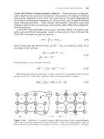
interstitial solutes in crystalline materials that lie in the interstices between larger
substitutional atoms, as, for example, carbon atoms in body-centered cubic (b.c.c.)
Fe, as illustrated in Fig.
8.8.
In such a system, carbon atoms can be added or
removed independently in a dilute solution.
When a network constraint is present,
NC
YdN,
=

0
u
i=l
(2.30)
2.2:
LINEAR IRREVERSIBLE
THERMODYNAMICS
31
Solving Eq.
2.30
for
dNNC
and putting the result into Eq.
2.3
yields
N,-l
Tds
=
du
+
dw
-
C
(pi
-
PN,)
dci
i=l
(2.31)
Starting with

Eq.
2.31
instead
of
Eq.
2.3
and repeating the procedure that led
to Eq.
2.15,
the conjugate force for the diffusion of component
i
in a network-
constrained crystal takes the new form
4
Fi
=
-v
(Pi
-
PN,)
(2.32)
The conjugate force for the diffusion of a network-constrained component
i
there-
fore depends upon the gradient of the difference between the chemical potential
of component
i
and
N,
rather than on the chemical potential gradient of compo-

nent
i
alone. If in the case of substitutional diffusion by the vacancy exchange
mechanism, the vacancies are taken as the component
N,,
the driving force for
component
i
depends upon the gradient of the difference between the chemical po-
tential of component
i
and that of the vacancies.
The difference arises because,
during migration, a site’s state changes from occupancy by an atom of type
i
to
occupancy by a vacancy. This result has been derived and extended by Larch6 and
Cahn, who investigated coherent thermomechanical equilibrium in multicomponent
systems with elastic stress fields
[l-41.
In the development above, the choice of the N,th component in a system un-
der network constraint system is arbitrary.
However, the flux of each component
in Eq.
2.21
must be independent of this choice
[3, 41.
This independence imposes
conditions on the
Lap

coefficients. To demonstrate, consider a three-component
system at constant temperature in the absence
of
an electric field, where compo-
nents
A,
B,
and
C
correspond to
i
=
1,
2,
and
3,
respectively. If component
C
is
the N,th component, Eqs.
2.21
and
2.32
yield
fA
=
-LAAv(PA
-
PC)
-

LABV(PB
-
PC)
JB
=
-LBAv(PA
-
~c)
-
LBBv(PB
-
~c)
fc
=
-LCAV(PA
-
~c)
-
LCBV(PB
-
~c)
(2.33)
On the other hand, if
B
is the N,th component,
+
JL
+
=
-LAA~(PA

-
PB)
-
LAC~(PC
-
PB)
JA
=
-LBA~(PA
-
PB)
-
LBC~(PC
-
PB)
&
=
-LCAV(PA
-
PB)
-
~ccv(pc
-
PB)
Because
$
must be the same as
<
and the gradient terms are not necessarily zero,
Eqs.

2.33
and
2.34
imply that
(2.34)
LAA
+
LAB
+
LAC
=
0
LBA
+
LBB
+
LBC
=
0
LCA
+
LCB
+
LcC
=
0
(2.35)
or generally,
NC
c

Lij
=
0
(2.36)
j=1
32
CHAPTER
2:
IRREVERSIBLE
THERMODYNAMICS:
COUPLED
FORCES
AND
FLUXES
If the lattice network defines the coordinate system in which the fluxes are mea-
sured, the network constraint requires that
i=l
and this imposes the further condition on the
Lij
that
C
Lij
=
0
(2.37)
(2.38)
2=1
In other words, the sum of the entries in any row or column
of
the matrix

L,,
is
zero.
The conjugate forces and fluxes that are obtained when the only constraint is a
network constraint are listed in Table
2.2.
However, there are many cases where
further constraints between the extensive quantities exist. For example, suppose
that component
1
is a nonuniformly distributed ionic species that has no network
constraint. Each ion will experience an electrostatic force due to the local electric
field, as well as a force due to the gradient in its chemical potential. This may be
demonstrated in
a
formal manner with Eq.
2.5,
noting that
dq
in this case is not
independent of
dcl
but, instead,
dq
=
qldq,
where
q1
is the electrical charge per
ion assuming that all electric current is carried by ions. Thus

dq
and
dcl
can be
combined in Eq.
2.5
into
a
single term
(p1
+ql@)dcl,
and when this term is carried
through the process leading to Eq.
2.15,
the ion flux,
A,
is found to be conjugate
to an ionic force
Fl
=
-V(p1+
q14)
(2.39)
The potential that appears in the total force expression is the sum of the chem-
ical potential and the electropotential of the charged ion. This total potential is
generally called the
electrochemical
potential.
Additional forces would be added to the chemical potential force if, for example,
the particle possessed a magnetic moment and a magnetic field were present. As

will be seen, many possibilities for total forces exist depending upon the types of
components and fields present.
Table
2.2:
Network-Constrained Components,
i
Conjugate Forces and Fluxes
for
Systems with
Quantity Flux Conjugate Force
Heat
J;k
-$VT
Component
i
-V
(pz
-
pN,)
=
-vQ.,
Charge
J:,
-V#
2.2.3
Introduction
of
the Diffusion Potential
Any potential that accounts for the storage of energy due to the addition of a
component determines the driving force for the diffusion of that component. The

2
2,
LINEAR IRREVERSIBLE THERMODYNAMICS
33
sum of all such supplemental potentials, including the chemical potential, appears
as the total conjugate force for a diffusing component and is called the
diffusion
potential
for that component and is represented by the symbol
@.’
The conjugate
force for the flux of component
1
will always have the form

FI
=
-Val
(2.40)
and thus for the special case leading to Eq.
2.39,
a1
=
p1
+
414
(2.41)
2.2.4
Onsager’s Symmetry Principle
Three postulates were utilized to derive the relations between forces and fluxes:

0
The rate of entropy change and the local rate of entropy production can be in-
ferred by invoking equilibrium thermodynamic variations and the assumption
of local equilibrium.
0
The entropy production is nonnegative.
0
Each flux depends linearly on all the driving forces.
These postulates do not follow from statements of the first and second laws of
thermodynamics.
Onsager’s principle supplements these postulates and follows from the statisti-
cal theory of reversible fluctuations
[5].
Onsager’s principle states that when the
forces and fluxes are chosen
so
that they are conjugate, the coupling coefficients are
symmetric:
Lap
=
Lp,
(2.42)
which simplifies the coupled force-flux equations and has led to experimentally
verifiable predictions
[6].
Furthermore, Eq.
2.42
guarantees that all the eigenvalues of Eq.
2.21
will be

real numbers. Also, the quadratic form in Eq.
2.23
together with Eq.
2.16
im-
plies that the kinetic matrix
(Lap)
will be positive definite; all the eigenvalues are
nonnegative
.a
Equation
2.42
can be rewritten
(2.43)
This equation shows that
the change in
flux
of
some
quantity caused
by
changing the
direct driving force for another is equal to the change
an
flux
of
the
second
quantity
caused

by
changing the driving force for the first.
These equations resemble the
Maxwell relations from thermodynamics.
7The potential is an aggregate
of
all reversible work terms that can be transported with the
species
i.
Using Lagrange multipliers, Cahn and Larch6 derive a potential that is a sum
of
the
diffusant’s elastic energy and its chemical potential
[4].
Cahn and Larch4 coined the term diffusion
potential
to
describe this sum.
Our
use
of
the term is consistent with theirs.
sPositive
definite
means that the matrix when left- and right-multiplied by an arbitrary vector will
yield
a
nonnegative scalar.
If
the matrix multiplied by

a
vector composed of forces is proportional
to a flux, it implies that the flux always has a positive projection on the force vector. Technically,
one should say that
Lap
is nonnegative definite but the meaning is clear.
34
CHAPTER
2
IRREVERSIBLE THERMODYNAMICS COUPLED FORCES AND FLUXES
The statistical-mechanics derivation
of
Onsager's symmetry principle is based
on microscopic reversibility for systems near equilibrium. That is, the time average
of
a correlation between
a
driving force
of
type
Q
and the fluctuations
of
quantity
/3
is identical with respect to switching
ct
and
/3
[6].

A demonstration of the role
of
microscopic reversibility in the symmetry of the
coupling coefficients can be obtained for a system consisting of three isomers,
A,
B,
and
C
[7,8].
Each isomer can be converted into either of the other two, without
any change in composition. Assuming a closed system containing these molecules at
constant temperature and pressure, the rate of conversion of one type into another
is proportional to its number, with the constant of proportionality being a rate
constant,
K (Fig.
2.1).
The rates at which the numbers of
A,
B,
and
C
change are
then

-
-
(KAC
+
KAB)NA
+

KBANB
+
KCANC
dNA
dt
-
dNB
=
KAB NA
-
(
KBC
+
KBA)NB
+
KCB Nc
dt
dNc
-
=KACNA
+
KBCNB
-
(KCA
+
KCB)NC
dt
(2.44)
At equilibrium, the time derivatives in
Eq.

2.44
vanish. Solving
for
equilibrium
in a closed system
(NA
+
NB
+
NC
=
Ntot) yields
K7 Ntot
Neq
=
K, Ntot Neq
-
Kp Ntot Neq
-
A
K,+K~+K,
-K,+K~+K,
-K,+K~+K~
(2.45)
where
K,
E
KBAKCA
+
KBAKCB

+
KCAKBC
Kp KCBKAB
+
KCBKAC
+
KABKCA
(2.46)
K7
E
KACKBC
+
KACKBA
+
KBCKAB
For the system near equilibrium, let
YA
be the difference between the number
of
A
and its equilibrium value,
YA
=
NA
-
N:q. Introducing this relationship and
similar ones for
B
and
C

into Eq.
2.44,
dYA
dt
-(KAc
+
KABIYA
+
KBAYB
+
KCAYC
(2.47)
-=
B
C
Figure
2.1:
Schematic conversion diagram for type
A,
B,
and
C
molecules.
2.2:
LINEAR IRREVERSIBLE THERMODYNAMICS
35
with similar expressions for
B
and
C.

chemical potential (Eq.
2.2)
near equilibrium (small
YA/N~~)
yields
If Henry's law is obeyed, the activity coefficient is constant and expanding the
(2.48)
Substituting Eq. 2.48 into Eq. 2.47 and carrying out similar procedures for
B
and
C,
These constitute a set of linear relationships between the potential differences
pz
-
p:q,
which drive the
Y,
toward equilibrium and their corresponding rates,
dY,/dt.
In terms of the Onsager coefficients, they have the form
=
LAAFA
+
LABFB
+
LACFC
%
=
LBAFA
+

LBBFB
+
LBCFC
(2.50)
3-
di
-
LCAFA
+
LCBFB
+
LCCFC
When microscopic reversibility is present in a complex system composed
of
many
particles, every elementary process in a forward direction is balanced by one in the
reverse direction. The balance of forward and backward rates is characteristic of the
equilibrium state, and
detailed balance
exists throughout the system. Microscopic
reversibility therefore requires that the forward and backward reaction fluxes in
Fig.
2.1
be equal,
so
that
KBA
-
Nip
=

Ka
- -
KBAKCA
+
KBAKCB
+
KCAKBC
KAB NEq Kp KCBKAB
+
KCBKAC
+
KABKCA

KCB
-
NB
=
Kp
=
KCBKAB
+
KCBKAC
+
KABKCA
KBC
Nzq
K-, KACKBC
+
KACKBA
+

KBCKAB

KAC
-
N~
=
K-r
=
KACKBC
+
KACKBA
+
KBCKAB
KCA Nip Ka KBAKCA
+
KBAKCB
+
KCAKBC
Comparison of Eq. 2.50 with Eqs. 2.49 and 2.51 shows that
L,,
=
L,,
and therefore
demonstrates the role of microscopic reversibility in the symmetry of the Onsager
coefficients. More demonstrations of the Onsager principle are described in Lifshitz
and Pitaerskii
[6]
and in Yourgrau et al.
[8].
Solving Exercise 2.5 shows that the products of the forces and reaction rates in

Eq. 2.49 appear in the expression for the entropy production rate for the chemical
reactions. The forces and reaction rates are therefore conjugate, as expected.

-
eq
(2.51)
-
-
Bibliography
1.
F.C. Larch6 and
J.W.
Cahn.
A
linear theory
of
thermochemical equilibrium of solids
under stress.
Acta
Metall.,
21(8):1051-1063,
1973.
36
CHAPTER
2:
IRREVERSIBLE
THERMODYNAMICS
COUPLED
FORCES
AND

FLUXES
2.
F.C. Larch6 and J.W. Cahn. A nonlinear theory
of
thermomechanical equilibrium
of
solids under stress.
Acta Metall.,
26(1):53-60, 1978.
3.
J.W.
Cahn and F.C. Larch& An invariant formulation of multicomponent diffusion in
crystals.
Scripta Metall.,
17(7):927-937, 1983.
4.
F.C. Larch6 and J.W. Cahn. The interactions
of
composition and stress in crystalline
solids.
Acta Metall.,
33(3):331-367, 1984.
5.
L. Onsager. Reciprocal relations in irreversible processes.
11.
Phys. Rev.,
38( 12):2265-
2279, 1931.
6.
E.M.

Lifshitz and L.P. Pitaevskii.
Statistical Physics, Part
1.
Pergamon Press, New
York,
3rd
edition,
1980.
See pages
365ff.
7.
K.
Denbigh.
The Principles
of
Chemical Equilibrium.
Cambridge University Press,
New York, 3rd edition,
1971.
8.
W. Yourgrau,
A.
ven der Merwe, and
G.
Raw.
Treatise on Irreversible and Statistical
Thermophysics.
Dover Publications, New York,
1982.
EXERCISES

2.1 Using an argument based on entropy production, what can be concluded
about the algebraic sign of the electrical conductivity?
Solution.
If
electronic conduction is the only operative process in a material at constant
T,
then
Eq.
2.15 reduces to
TU=-&.Vc$
(2.52)
Using Ohm's law,
&
=
-pV4,
TU
=
p
10c$l2
(2.53)
Because
U
2
0
and
lVc$12
is
positive,
p
must be positive.

2.2
An isolated bar
of
a good electrical insulator contains
a
rapidly diffusing
unconstrained solute (i.e., component
1).
Impose a constant thermal gradient
along the bar, and find an expression for its thermal conductivity when the
system reaches a steady state. Assume that no solute enters or leaves
the
ends
of
the bar. Express your result in terms of any
of
the
Lap
coefficients in
Eq.
2.21
that are required.
Solution.
Using a similar method as the development that led to
Eq.
2.29, the relevant
linear force-flux relations are
JQ
=
LQQFQ

+
LQ~FI
Ji
=
LQFQ
+
LiFi
(2.54)
The cross effect between the thermal and diffusion currents causes a redistribution of
the unconstrained solute until
a
steady-state distribution
is
reached. In this condition
51
=
0
and, therefore,
F1
=
-FQ(L~Q/L~~).
Putting this result into
Eq.
2.54 then
vields
The expression for
K
is similar to
Eq.
2.29,

where electrical charge rather than compo-
nent
1
was forced into
a
steady-state distribution by the thermal flux.
2.3
A
common device used to measure temperature differences is the thermocou-
ple in Fig.
2.2.
Wires
of
metals
A
and
B
are connected with their common
EXERCISES
37
I
junction at the temperature
T
+AT and the opposite ends connected to the
terminals of a potentiometer maintained at temperature
T.
The potentiome-
ter measures a voltage,
+AB,
across terminals

1
and
2
under conditions where
no electric current is flowing. This voltage is then a measure of AT. Explain
this effect, known as the
Seebeck effect,
in terms of relevant forces and fluxes.
Potentiometer
1
I
I
+Temperature
T
I
I
I
1
I
I
L
- - - -
-
,-Temperature
T+AT
Figure
2.2:
Thermocouple
composed of metals
A

and
B
with
a
junction
at
one end.
Solution.
The appropriate force-flux equation for this case is
1
dT
d4
Jq
=
L¶QFQ
+
Lq,Fq
=
-L,Q?;~
-
L
-
"
dx
(2.56)
where, to a good approximation,
2
measures the distance along the wire. Setting
Jq
=

0,
d4
LYQ
dT
L,,
T
(2.57)
The potentials at
1
and 2 relative to the potential at the junction are determined by
integrating Eq.
2.57
along each wire. They will difFer because the
A
and
B
wires possess
different values of the coefficients
L,Q
and
Lyq,
~AB
is then the difference between
these two potentials.
2.4
Figure
2.3
depicts an apparatus at constant uniform temperature. The bat-
tery drives an electrical current around the circuit. Heat is absorbed at one
AIB

junction and emitted at the other. Explain this phenomenon, known as
the
Peltier effect,
in terms of relevant forces and fluxes.
A
Figure
2.3: Peltier
effect
apparatus
coiriposed
of
metnl
wires
A
and
H
38
CHAPTER
2:
IRREVERSIBLE
THERMODYNAMICS:
COUPLED
FORCES
AND
FLUXES
Solution.
Both heat and electrical charge currents will be present in the wire, and the
generalized linear relationships are therefore
1
dT d4

JQ
=
LQQFQ
+
LQ,F,
=
-LQQ
-
LQ,~
T
dx
X
1
dT d4
5,
=
L,QFQ
+
LqqFq
=
-Lq4
-
Lqq-
T
dx dx
(2.58)
(2.59)
where, to a good approximation,
z
measures distance along the wires. Because

dT/dz
=
0,
JQ
=
-Jq
LQ4
(2.60)
Lqq
Equation
2.60
shows that the electrical current will drive a heat current along each wire
by an amount dependent upon the coupling coefFicient
LQ,
and the direct coefficient
L,,.
These coefFicients will have different values in the
A
and
B
wires, and therefore
heat will accumulate (and be emitted) at one junction and be absorbed at the other.
2.5
Show that products of the "forces" [i.e., the quantities
(p:"
-
pi)],
and the
rates of reaction (i.e., the
dY,/dt)

which are present in Eq. 2.49 appear in the
expression for the rate at which entropy is produced by the corresponding
reactions. These quantities are therefore conjugate to one another just as are
the conjugate forces and fluxes in Table
2.1.
Obtain a general expression for the rate
at
which entropy
is
produced:
the reactions are taking place in a container maintained
at
constant
temperature and pressure.
0
The surroundings may be regarded as a reservoir at constant tempera-
ture and pressure.
0
It may be necessary to transfer a quantity of heat,
dQ,
from the reservoir
into the system in order
to
maintain constant temperature in the system;
the total entropy change of the system plus reservoir,
dS',
will then be
dQ
dS'
=

dS
-
-
T
(2.61)
where
dS
and
-dQ/T
are the entropy changes of the system and
sur-
roundings, respectively. For the system,
du
=
dQ
-
PdV,
and therefore
(2.62)
TdS
-
02.4
-
PdV
T
dS'
=
0
Note that
6

=
U
+
PV
-
TS,
and applying the constant temperature
and pressure condition,
(2.63)
0
Equation 2.63,
Q
=
U
+
PV
-
TS,
and Eq.
2.1
can be combined in the
expression for the rate of entropy production:
T,P
i
(2.64)
EXERCISES
39
Solution.
From Eq.
2.64,

But
dNi/dt
=
dYi/dt,
and therefore
Suppose that the system is
at
equilibrium with all three species at their equilibrium
chemical potentials.
We
then make small changes in their numbers subject
to
the
conservation condition
NA
+
NB
+
Nc
=
N~''
Since in general for a system at constant
T
and
P,
dG
=
PA
dNA
+

/.LB
dNB
+
pc
dNc
the change in free energy of the system at equilibrium will be
dG
=
p:
dNA +/.LzdNB +pL',4dNc
=
0
Since
Y,
=
Ni
-
Nteq,
py
dYA
-t
pz
dYB
f
pz
dYc
=
0
and
adding Eqs.

2.66
and
2.71
then produces
(2.67)
(2.68)
(2.69)
(2.70)
(2.71)
(2.72)
CHAPTER
3
DRIVING FORCES AND FLUXES FOR
DIFFUSION
Fluxes of chemical components may arise from several different types of driving
forces. For example, a charged species tends to flow in response to an applied
electrostatic field; a solute atom induces a local volume dilation and tends to flow
toward regions of lower hydrostatic compression. Chemical components tend to
flow toward regions with lower chemical potential. The last case-flux in response
to a chemical potential gradient-leads to Fick’s first law, which is an empirical
relation between the flux of a chemical species,
$,
and its concentration gradient,
Vci
in the form
$
=
-DVci,
where the quantity
D

is termed the
mass
diffusivity.
Because different driving forces can arise for a chemical species and because the
mechanisms of diffusion comprising the microscopic basis for
D
are essentially inde-
pendent of the driving force, all the driving forces can be collected and attributed
to the generalized
diffusion potential,
CJ,
introduced in Chapter
2.
The flux of a component in a solution can be complicated because components
cannot always diffuse independently. This complication necessitates the introduc-
tion of different types of diffusion coefficients defined in specified reference frames
to distinguish different diffusion systems.
3.1
DIFFUSION IN PRESENCE
OF
A CONCENTRATION GRADIENT
If a concentration gradient exists in a single phase at uniform temperature that
is free of all other fields and any interfaces, that component’s diffusion potential
is identical to its chemical potential. The gradient in this potential is the driving
Kinetics
of
Materials.
By
Robert
W. Balluffi, Samuel

M.
Allen, and W. Craig Carter.
41
Copyright
@
2005
John Wiley
&
Sons, Inc.
42
CHAPTER
3
DRIVING
FORCES
AND
FLUXES
FOR
DIFFUSION
force for diffusion. A diffusional flux proportional to the diffusion potential gradient
will then arise,
as
discussed in Chapter
2.
However, it is much easier to determine
a concentration gradient by experiment than a diffusion potential gradient. It is
therefore convenient to use a thermodynamic model of the solution to express the
chemical-potential gradient in terms of a concentration gradient. The result is a
diffusional flux proportional to the concentration gradient. The factor coupling the
flux and concentration gradient is termed a
diffusivity

(or
diffusion coefficient),
D,
so
that Fick’s first law in the form
J’=
-DVc
(3.1)
applies. The flux and corresponding diffusivity in this relationship must always be
specified relative to a particular
reference frame
(coordinate system)
[I,
21.
3.1.1
Self-Diffusion: Diffusion in the Absence
of
Chemical Effects
During self-diffusion in a pure material, whether a gas, liquid,
or
solid, the compo-
nents diffuse in a chemically homogeneous medium. The diffusion can be measured
using radioactive tracer isotopes
or
marker atoms
that have chemistry identical to
that
of
their stable isotope. The tracer concentration is measured and the tracer
diffusivity (self-diffusivity) is inferred from the evolution of the concentration pro-

file.
Figure
3.1
shows a diffusion couple containing a concentration gradient of the
tracer atoms that could be used for this purpose.
For
a crystal where self-diffusion
takes place by the vacancy-exchange mechanism, the Fick’s law flux equation can
be derived.l Such a crystal is network-constrained and has three components-
inert atoms, radioactive atoms, and vacancies
[3].
Planes of atoms provide a local
reference frame to quantify the fluxes of these components by allowing the count
of the number of atoms that cross a unit area of crystal plane per unit time. The
crystal remains rigidly fixed during self-diffusion, and therefore these planes con-
stitute a convenient single reference frame, called the crystal frame,
or
C-frame,
for measuring flux. At constant temperature, with vacancies chosen as the N,th
-W
0
W
Distance
-
Figure
3.1:
Diffusion couple for measuring self-diffusion in pure material.
A
small
coriceritratioii of

a
radioactive isotope
of
component
1.
c4,,
is
present initially on the left
side of the couple. During diffusion, the radioactive particles will diffuse in the chemically
homogeneous couple
and
become inteririixed with the inert particles.
’The vacancy exchange mechanism is described in Section
8.1.2.
3
1.
CONCENTRATION GRADIENTS AND DIFFUSION
43
component, Eq.
2.21
combined with Eq.
2.32
takes the form (for one-dimensional
isotropic diffusion)
where the star indicates the radioactive species, and the superscript
C
indicates
that the flux of
i
is measured in a C-frameS2 These equations are derived from

the vacancy-exchange mechanism; every forward jump
of
an atom occurs via a
backward jump of a vacancy. The vacancies are assumed
to
be in thermodynamic
equilibrium throughout, and therefore
pv
=
0.3
c1
+
c.1
+
cv
=
A,
where
A
is a
constant and typical vacancy atomic fractions are less than
potentials
of
species
1
and
1
are given by Eq.
2.2
with Raoultian

y1
=
y*1
=
1).
Therefore,
dpi/dx
=
kTdlnci/dx. Because of the
uniform vacancy equilibrium,
c1
+
c.1
=
A
-
cv
is also uniform.
become
The chemical
behavior (i.e.,
assumption of
Equations
3.2
Lq*1 L*11 dcq
-
ax
J$
=
-

IcT
[-,
-
Finally, because
J$
=
0
and
JY
+
JZ
=
0,
(3.3)
Equation
3.4
shows that the self-diffusion
of
the radioactive tracers obeys Fick's
law with
a
self-diffusivity designated by
*D.
'The vector notation is dropped when there is only one spatial dimension. Unless indicated
otherwise, the diffusion is assumed to be isotropic in this chapter. Anisotropic diffusion is treated
in Section
4.5.
3The vacancy chemical potential is defined by
pv
=

(aG/aNv)~,p,
that is, by the free-energy
increase of a large system when a vacancy is created at a source such
as
a dislocation
or
a
grain boundary. Dislocations act
as
vacancy sources as they climb in one direction and as sinks
(i.e., negative sources), as they climb in the other. Throughout this book we generally refer
to
vacancy sources with the understanding that source and sink behavior are complementary (see
Section
11.4).
When this free-energy change is zero (i.e.,
pv
=
0),
the system will be in
a
minimum
free-energy state with respect to vacancy formation. The vacancy concentration at the source is
then in local equilibrium. Assuming that
pv
is uniformly zero in a system requires an adequate
density of vacancy sources.
44
CHAPTER
3:

DRIVING FORCES AND FLUXES FOR DIFFUSION
3.1.2
Self-Diffusion
of
Component
i
in a Chemically Homogeneous Binary
Solution
In Section
3.1.1,
the self-diffusivity was obtained for a diffusion couple composed
of a chemically pure material but with gradients of an isotope of that material. In
this section we discuss self-diffusion of an isotopic species in a chemically homo-
geneous binary solution consisting of atoms of types
1
and
2
in the presence of a
concentration gradient of the isotope.
The self-diffusion of component
1
in such a system is measured by studying the
diffusion of a radioactive isotope tracer of component
1
(i.e.,
q)
under the condition
that while there is a gradient in the tracer's concentration,
c*1,
the sum

(c1
+
cq)
and
c2
are both uniform. A possible diffusion couple is shown in Fig.
3.2.
Considering
Eq.
2.21
in a case in which diffusion occurs in a crystal by the
vacancy exchange mechanism, there are four components,
c1,
c*1,
c2,
and
cv.
Be-
cause the crystal remains fixed during the diffusion, the C-frame is again used for
measuring the flux. The system is chemically homogeneous,
so
Again, a Fick's-law expression is obtained for the self-diffusion of the radioactive
component. The self-diffusivity of component
1
in a binary system of uniform
chemical composition is designated by
*D1
to distinguish it from the self-diffusivity
of
a

pure material,
*D.
t
-m
0
W
Distance
+
Figure
3.2:
During diffusion,
a
cq
gradient develops in the chemically homogeneous material.
Diffusion couple for nietlsuring solute self-diffusion in
a
binary systein.
3.1.3
Diffusion
of
Substitutional Particles in a Chemical Concentration
Gradient
When a solute of type
i
diffuses on substitutional sites in an inhomogeneous binary
solution, both the solute particles and host particles interdiffuse on the substitu-
tional sites.
If
one species diffuses more quickly than the other, the region initially
richer in that species loses net

mass
and contracts. On the other hand, the region
initially richer in the more slowly diffusing species gains net
mass
and expands.
This process, which establishes a
mass
flow in the system, is known
as
the
Kirk-
endall
efSect
after
E.
Kirkendall, who along with A. Smigelskas first observed it in
crystalline metals
[4].
3
1
CONCENTRATION GRADIENTS AND DIFFUSION
45
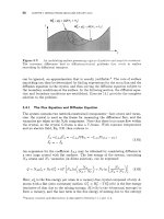
Description of the Diffusion in a
Local
C-Frame. Figure
3.3
illustrates
a
crystalline
binary system in which interdiffusion occurs along

x
by
a
vacancy mechanism. The
crystal is no longer fixed in structure as during self-diffusion but
is
flowing due to
the Kirkendall effect, and its local planes are moving with
a
velocity,
~(x).
with
respect to the ends
of
the sample. Although no unique C-frame exists throughout
the diffusing crystal, a local C-frame with
a
small inert marker particle to indicate
its origin can be fixed to any plane as illustrated. The distribution of the faster-
diffusing solute
(i
=
1)
is also shown in Fig.
3.3a.
If
the diffusion fluxes are measured
at any point in the diffusion zone with respect to its local C-frame, the constraint
condition associated with the vacancy mechanism requires that the fluxes satisfy
In the Kirkendall effect, the difference in the fluxes of the two substitutional

species requires
a
net flux of vacancies. The net vacancy flux requires continuous
net vacancy generation on one side of the markers and vacancy destruction on
the other side (mechanisms of vacancy generation are discussed in Section
11.4).
Vacancy creation and destruction can occur by means of dislocation climb and is
illustrated in Fig.
3.3b
for edge dislocations. Vacancy destruction occurs when
atoms from the extra planes associated with these dislocations fill the incoming
vacancies and the extra planes shrink (i.e the dislocations climb as on the left side
in Fig.
3.3b
toward which the marker is moving). Creation occurs by the reverse
process, where the extra planes expand as atoms are added to them in order to
form vacancies, as on the right side of Fig.
3.3b.
This contraction and expansion
causes
a
mass flow that is revealed by the motion
of
embedded inert markers. as
indicated in Fig.
3.3
[4].
jii
+
Tc

+
jii
=
0
2v
Figure
3.3:
Schematic illustration
of
the Kirkeridall effect in
a
binary crystalline material
diffusing by the vacancy mechanism. The sketch illustrates dislocation motion at, some t,ime
aft>er the diffusion couple’s initial condition.
(a)
Concentration vs. distance profile
in
t,he
diffusion zone. An embedded inert marker is present moving with the velocity.
v.
and fluxes
in the local C-frame associated with t,he marker are iridica.ted.
(b)
Local arrarigemerit
of
at,om plaries across the diffusion zone near the marker. Arrows indicate clirrih movements of
niiinerous edge dislocations that occur when there is
a
net diffusion
of

vacancies from right
to
left,.
46
CHAPTER
3:
DRIVING
FORCES
AND
FLUXES
FOR
DIFFUSION
In this process, the net flux of substitutional atoms across the interface plane
results in local volume changes (i.e., as a crystal plane is removed by climb, the
crystal contracts in a direction normal to the plane). However, free expansion
in directions parallel to the interface plane is constrained by the specimen ends,
where significant diffusion has not occurred, and by the coherence of the interface
between the expanding and contracting regions. Therefore, dimensional changes
parallel to the interface (i.e., normal to the diffusion direction) are restricted, and
in-plane compatibility stresses are generated.
No
out-of-plane compatibility stresses
develop because the diffusion couple can expand freely in the diffusion direction.
In diffusion specimens that have a relatively narrow diffusion zone compared
to the extent of the specimen in the diffusion direction, compatibility stresses are
pure shear stresses, and if the stresses exceed the crystal's yield stress, the onset of
plastic flow enables the cross section
of
the diffusion specimen to remain ~onstant.~
The substitutional binary alloy diffusion illustrated in Fig.

3.3
is discussed in a
treatment pioneered by Darken
[6]
(see also Crank's book
"71).
The system has three
components, species
1,
species
2,
and vacancies, and is assumed to be at constant
pressure and temperature with sites that can only be created or destroyed at sources
(i.e., the system is network constrained except
at
dislocations or interfaces). The
fluxes are obtained from Eqs.
2.21
and
2.32:
JF
=
LiiFi
+
LizF2
8%
d@2
d(P1
-
Pv)

-
L12
d(P2
-
PV)
=
-L11-
-LIZ
=
-L11
(3.7)
dX
dX
dX dX
Jg
=
~521~1
+
L22F2
d(P2
-
Pv)
dX
-
L22
8%
332
d(P1
-
PV)

=
-L21-
-
L22-
=
-L21
dX
dX dX
and
J$
=
-(Jf
+
J,C)
by Eq.
3.6.
Assumption of local equilibrium permits the Gibbs-Duhem relation to be written
(3.8)
A net vacancy flux develops in a direction opposite that of the fastest-diffusing
species (species
1
in Fig.
3.3).
Nonequilibrium vacancy concentrations would de-
velop in the diffusion zone if they were not eliminated by dislocation climb. How-
ever, under usual conditions it is expected that a sufficient density of dislocations
will be present to maintain the vacancy concentration near equilibrium
IS].
It
can therefore be assumed, to a good approximation, that

pv
=
0,
and therefore
Vpv
=
0
everywhere in the diffusion zone. Using Eqs.
3.7
and
3.8
with
Vpv
=
0
yields
(3.9)
4When the faster-diffusing component is diffused from the vapor phase into a thin sheet, and the
diffusion zone is relatively wide compared to the sheet thickness, the constraints on the expansion
parallel to the diffusion interface are greatly reduced. Large specimen expansions normal to the
diffusion direction have then been observed
[5].
3.1
CONCENTRATION GRADIENTS AND DIFFUSION
47
The chemical potential gradients can be related to concentration gradients using
pi
=
p:
+

kTln(yi(R)ci)
(3.10)
which is obtained by combining
Eq.
2.2
with
Eq.
A.12, giving the result
dX
(3.11)
The local volume expansion arising from the local change of composition contributes
to diffusion via the derivative of the average site volume
(R).5
The derivative of
71
is the contribution associated with the nonideality of the solution. Putting
Eq.
3.11
into
Eq.
3.9 yields a flux that is proportional to the concentration gradient:
This is a form of Fick’s law for a chemically inhomogeneous material where the
intrinsic diffusivity, designated by D1, measures the flux in the local C-frame.
A similar procedure for component
2
yields an analogous Fick’s-law expression,
The self-diffusivity of species
1
in a chemically homogeneous solution of concen-
tration c1, corresponding to *D1 in

Eq.
3.5, can be compared with the intrinsic
diffusivity of the same species in a chemically inhomogeneous solution at the same
concentration, corresponding to
D1
in
Eq.
3.12. Typically, in addition to the ap-
proximation of a concentration-independent average site volume
(O),
it is reasonable
to assume that the coupling (off-diagonal) terms, Ll2/c2 and Ll*l/c*l in
Eqs.
3.5
and
3.12,
are small compared with the direct term Lll/cl. In this approximation,
J,C
=
-Dzdca/d~.
(3.13)
The primary difference between
D1
and
*D1
is a thermodynamic factor involving
the concentration dependence of the activity coefficient of component
1.
The ther-
modynamic factor arises because mass diffusion has

a
chemical potential gradient
as
a
driving force, but the diffusivity is measured proportional to a concentration
gradient and is thus influenced by the nonideality of the solution. This effect is
absent in self-diffusion.
At
this point it has been shown that the fluxes of species
1
and
2
can be described
by Fick’s-law expressions involving two different intrinsic diffusivities, D1 and
02,
in a local coordinate system (local C-frame) fixed to the lattice plane through which
flux is measured. However, because of the Kirkendall effect, these planes (reference
frames) move normal to one another
at
different rates in a nonuniform fashion,
and this description is therefore not useful for describing the diffusion throughout
the specimen. When there is no change in the total specimen volume, the overall
diffusion that occurs during the Kirkendall effect can be described in terms of
a single diffusivity (the interdiffusivity) measured in a single reference frame (a
volume-fixed) frame.
5This expansion can usually be described by
Vegard’s
law
in the
form

ezj
-
e:j
=
Tz3
(c
-
CO);
et3
is the strain due
to
a concentration change, and the six
Tz3
are the Vegard coefficients.