Kinetics of Materials - R. Balluff_ S. Allen_ W. Carter (Wiley_ 2005) Episode 6 pot

206
CHAPTER
8.
DIFFUSION
IN
CRYSTALS
The hysteresis loop will therefore appear as a line of negligible width and slope
1/SR
as in Fig.
8.24a.
Negligible internal friction therefore occurs.
U U
U
Figure
8.24:
Frequency dependence
of
anelastic behavior.
(a)
w~
<<
1.
(b)
WT
>>
1.
(c)
WT
=
1.
(b)

When
wt
>>
1,
EI
=
Suu0
and
€2
=O
(8.172)
The hysteresis loop will therefore appear again as a line of negligible width but
with a larger slope,
as
in Fig.
8.246.
Negligible internal friction occurs.
(c)
When
wt
=
1,
(8.173)
The hysteresis loop will therefore appear as in Fig.
8.24~.
The slope of the dashed
line is
(8.174)
SR
-

SU
and
EZ
=
~u,
SR
+
SU
=
2uo
1
-
uo
El
(SRfSU)/2
_-
and the width
of
the loop
at
u
=
0
is
2EZ
=
(SR
-
sU)Uo
(8.175)

Also,
because the strain lags behind the stress, the direction of traversal of the
loop must be as indicated. In this situation, maximum internal friction occurs.
8.22
Describe in detail how to determine the diffusivity of
C
in b.c.c. Fe using a
torsion pendulum. Include all
of
the necessary equations.
See Section
8.3.1
and Fig.
8.8,
where
C
atoms in sites
1,
2,
and
3
expand
the crystal preferentially along
z,
y,
and
z,
respectively.
Solution.
Using a torsion pendulum, find the anelastic relaxation time,

T,
by measuring
the frequency of the Debye peak,
up,
and applying the relation
W~T
=
1. Having
T,
the
relationship between
T
and the
C
atom jump frequency
r
is found by using the procedure
to find this relationship for the split-dumbbell interstitial point defects in Exercise
8.5.
Assume the stress cycle shown in Fig.
8.16
and consider the anelastic relaxation that
occurs just after the stress
is
removed. A
C
atom in a type
1
site can jump into two
possible nearest-neighbor type

2
sites
or two possible type
3
sites. Therefore,
-
dcl
=
-4r/cl
+
2r’c2
+
2r/c3
dt
(8.176)
Because
c1
+
c2
+
c3
=
ctot
=
constant,
(8.177)
EXERCISES
207
which may be integrated to obtain
8.23

[
c;]
[
c;]
-6r’t
ci(t)
-
-
=
~(0)
-
-
=e
(8.178)
The relaxation time
is
then
T
=
1/(6l?),
and because the total jump frequency
is
r
=
4l?,
T
=
2/(3r).
According to Eq.
7.52,

DZ
=
rr2/6
because
f
=
1,
and because
r
=
a/2,
DI
=
ra2/24.
Substituting for
r,
(8.179)
Finally, insert the experimentally determined value of
T
into Eq.
8.179
to obtain
DI
Under equilibrium conditions in a stressed b.c.c. Fe crystal, interstitial
C
atoms are generally unequally distributed among the three types of sites iden-
tified in Fig.
8.8b.
This occurs because the C atoms in sites
1,

2,
and
3
in
Fig.
8.8b
expand the crystal preferentially along the
2,
y,
and
z
directions,
respectively. These directions are oriented differently in the stress field, and
the
C
atoms in the various types of sites therefore have different interaction
energies with the stress field. In the absence of applied stress, this effect does
not exist and all sites are populated equally. In Exercise
8.22
it was shown
that when the stress on an equilibrated specimen is suddenly released, the re-
laxation time for the nonuniformly distributed
C
atoms to achieve a random
distribution,
T,
is
T
=
2/(3r),

where
r
is the total jump frequency of a
C
atom in the unstressed crystal.
Show that when stress is suddenly applied to an unstressed crystal, the relax-
ation time
for
the randomly distributed C atoms to assume the nonrandom
distribution characteristic
of
the stressed state is again
T
=
2/(3r).
Assume the energy-level system for the specimen shown in Fig.
8.25.
Write the kinetic equations for the rates of change of the concentrations
of the interstitials in the various types of sites and solve them subject
to the appropriate initial and final conditions. Assume that the barri-
ers to the jumping interstitials shown in Fig.
8.25
are distorted by the
differences in the site energies (indicated in Fig.
8.21).
Figure
8.25:
atom in sites
1,
2,

or
3
illustrated in Fig.
8.8.
Energy-level diagram
for
a
stressed
b.c.c.
specimen containing an interstitial
Solution.
Let
c1,
c2,
and
c3
be the concentrations
of
interstitials occupying sites
of
types
1,
2,
and
3,
respectively.
Also,
c1 +c2 +c3
=
ctot

=
constant. Since an interstitial
208
CHAPTER
8:
DIFFUSION
IN
CRYSTALS
in a given type of site can jump into two
sites
of each other type,
dci
dt
dc2
dt
-
=
-
2
(rL
+
rL3
+
rL)
c1
+
2
(rL1
-
rL)

c2
+
2r’3+1~t0t
-
=
-
2
(rL1
+
rL3
+
rL2)
c2
+
2
(rL
-
r;,2)
c1
+
2r$-2~tot
(8.180)
If
the barrier to the jump of an interstitial between two sites of differing energy is
deformed as indicated in Fig. 8.21, the information given in Fig. 8.25 may be used to
derive expressions for the various jump rates that appear in the coefficients
of
Eq. 8.180.
Neglecting small differences in the entropies of activation in the presence and absence
of stress, and expanding Boltzmann factors

of
the form
exp[-U,,,/(kT)]
to first order
so
that
exp[-U,-,/(kT)]
=
1
+
Ut-J/(kT),
r;-2
=
r’
(1
-
w)
=
r/
(1
-
w)
r;+l
=
r’
(1
+
W-J
rLl
=

r’
(1
+
w)
r;,3
=
r’
(1
-
h)
=
r’
(1
+
-
h)
r;,,
=
r’
(1
-
+
*)
2kT 2kT 2kT
(8.181)
where
I?’
is the jump rate between any two adjacent sites in the absence of stress. Equa-
tion 8.180 is a pair of simultaneous linear first-order equations with constant coefFicients.
The initial and final conditions are

c1
(m)
=
ci‘
c2(m)
=
c;q
(8.182)
where
el( )
and
c2(m)
are the final equilibrium concentrations reached at long times
in the presence of the applied stress. In view of the symmetry of Eqs. 8.180, we try
Ctot
Cl(0)
=
c2(0)
=
-
3
Cl(t)
=
(f
-
‘p>
e-k‘t
+
.;‘
c2(t)

=
(f
-
c;~)
e-“lt
+
c‘lq
(8.183)
which satisfy the conditions in Eq. 8.182. Direct substitution shows that Eqs. 8.183
indeed satisfy Eqs. 8.180 when higher-order terms involving products of the small quan-
tities
Ut-j/(kT)
are neglected and
k‘
=
6r’
c‘lq
=
-
I+-+-)
Ul-2
u1-3
3
(
3kT 3kT
(8.184)
1
2u1+2
3kT
+

3kT
This shows that relaxation to the equilibrium distribution occurs exponentially with
a
relaxation time
T
=
1/(6r’).
Since
=
4r’,
where
r
is the total jump frequency in the
unstressed crystal,
7
=
2/(3r).
Finally, the equilibrium concentrations obtained in Eqs. 8.184 from the kinetic equations
agree with those obtained using equilibrium statistical mechanics. In the three-level
system in Fig. 8.25, the occupation probability for level
1
is
Since c1
=
ctotpl, the result for
CI
is the same as that given by Eq. 8.184. Similar
agreement is obtained for
c2.
CHAPTER

9
DIFFUSION ALONG CRYSTAL
IMPERFECTIONS
Experiments demonstrate that along crystal imperfections such as dislocations, in-
ternal interfaces, and free surfaces, diffusion rates can be orders
of
magnitude faster
than in crystals containing only point defects. These line and planar defects pro-
vide
short-circuit diffusion paths,
analogous to high-conductivity paths in electrical
systems. Short-circuit diffusion paths can provide the dominant contribution to
diffusion in a crystalline material under conditions described in this chapter.
9.1
THE DIFFUSION SPECTRUM
IN
IMPERFECT CRYSTALS
Rapid diffusion along line and planar crystal imperfections occurs in a thin region
centered on the defect core. For a dislocation, the region is cylindrical, roughly two
interatomic distances in diameter, and includes the “bad material” in the dislocation
core.’ For a grain boundary, the region is a thin slab, roughly two interatomic
distances thick, including the bad material in the grain boundary core. For a free
surface, this region is the first few atomic layers of the material
at
the surface. These
regions are very thin in comparison to the usual diffusional transport distances.
To
model the diffusion due to these imperfections, we replace them by thin slabs or
cylinders of effective thickness,
6,

possessing effective diffusivities which are much
larger than the diffusivity in the adjoining crystalline material. Table
9.1
lists the
Bad material
is disordered material in which the regular atomic structure characteristic of the
crystalline state
no
longer exists.
Good bulk
material
is free
of
line
or
planar imperfections.
Kinetics
of
Materials.
By
Robert W. Balluffi, Samuel
M.
Allen, and W. Craig Carter.
209
Copyright
@
2005
John Wiley
&
Sons, Inc.

210
CHAPTER
9
DIFFUSION ALONG CRYSTAL IMPERFECTIONS
Table
9.1:
Notation for Short-circuit Diffusivities
DD (undissoc) diffusivity along an undissociated dislocation core (i.e., a cylin-
der,
or
a
“pipe” of diameter,
6)
DD
(dissoc) diffusivity along a dissociated dislocation core (i.e., a cylinder,
or
a “pipe” of diameter,
6)
DB
diffusivity along
a
grain boundary (i.e., a slab of thickness,
6)
DS
DXL
diffusivity along
a
free surface (i.e., a slab of thickness,
6)
diffusivity in

a
bulk crystal free of line
or
planar imperfections
DL diffusivity in a liquid
notation to be used to describe the diffusivities in various regions of crystalline
materials containing line and planar imperfections.
Figure
9.1
presents self-diffusivity data for
*DD
(dissoc),
*DD
(undissoc),
*DB,
*Ds,
*DxL,
and
*DL,
for f.c.c. metals on a single Arrhenius plot. With the excep-
tion of the surface diffusion data, the data are represented by ideal straight-line
Arrhenius plots, which would be realistic if the various activation energies were
constants (independent of temperature). However, the data are not sufficiently
accurate or extensive to rule out some possible curvature, at least for the grain
boundary and dislocation curves, as discussed in Section
9.2.3.
Dislocations, grain boundaries, and surfaces can possess widely differing struc-
tures, and these structural variations affect their diffusivities to significant degrees.
If the defective core region is less dense or “looser” than defect-free material, or
if a defect possesses structurally “open” channels in its core structure, transport

will generally be more rapid along the defect, particularly in the open directions.
Some grain boundary structures can be represented by dislocation arrays, and their
boundary diffusivity can be modeled in terms of transport along the grain-boundary
0.6
0.8 1.0 1.2 1.4
1.6
1.8 2.0
Reduced
temperature,
T,,,
lT
Figure
9.1: Master Arrhenius plot of *DxL, *DD(dissoc), *D”(undissoc), *DB, *Ds,
and *DL characteristic
of
f.c.c. metals. Data for various f.c.c. metals have been normalized
by using
a
reduced reciprocal temperature scale,
(l/T)/(l/Tm)
=
T,/T.
All diffusivities
were derived from experimental data by assuming that all
6
=
0.5
nm.
From
Gjostein

[I].
9.1:
THE
DIFFUSION
SPECTRUM
211
dislocation cores. General grain boundary structures cannot support discrete local-
ized dislocations but, nevertheless, still act as short-circuit diffusion paths.
Short-circuit diffusion along grain boundaries has been studied extensively via
experiments and modeling. Because diffusion along dislocations and crystal sur-
faces is comparatively less well characterized, particular attention is paid to grain-
boundary transport in this chapter. However, briefer discussions of diffusion along
dislocations and free surfaces are also presented.
To
describe the effects of grain-boundary structure on boundary diffusion, it is
necessary to review briefly some important aspects of boundary structure. Addi-
tional details appear in Appendix B. It takes a minimum of five geometric pa-
rameters to define a crystalline interface. Three describe the crystal/crystal
mis-
orientation:
e.g., two to specify the axis about which one crystal is rotated with
respect to the other, and one for the rotation angle. The remaining two parameters
define the
inclination
of the plane along which the crystals abut at the interface.2
If the interface is a free surface, just two parameters are required to specify the
surface's inclination (unit normal). Crystal symmetries determine special values of
the parameters at which the interfacial energies take on extreme values. Depending
on the specific nature of a system with interfaces, some of the parameters may be
constrained and others free to vary as the system seeks

a
lower-energy state.
Small-angle grain boundaries
have crystal misorientations less than about
15"
and consist of regular arrays of discrete dislocations (Le., where the cores are sep-
arated by regions of defect-free material). As the crystal misorientation across the
boundary increases beyond about
15",
the dislocation spacing becomes
so
small
that the cores overlap and the boundary becomes a continuous slab of bad mate-
rial; these are called
large-angle boundaries.
Large-angle boundaries can be further
classified into singular boundaries, vicinal boundaries, and general b~undaries.~
An interface is regarded as
singular
with respect to
a
degree of freedom
if
it is
at a local minimum in energy with respect to changes in that degree of freedom. It
is therefore stable against changes in that degree of freedom.
A
vicinal interface
is an interface that deviates from being singular by a rela-
tively small variation of one or more of its geometric parameters from their singular-

interface values. A vicinal interface can therefore minimize its energy by adopting
a fit-misfit structure consisting of patches of the nearby minimum-energy singular
interface delineated by arrays of discrete interfacial dislocations or steps as illus-
trated in Figs. B.4 and
B.9.
These line defects serve to accommodate the relatively
small deviations of the vicinal interfaces from the singular interfaces.
A
general interface
is not energy-minimized with respect
to
any of its degrees
of freedom, and is far from any singular-interface values of the parameters that set
its degrees of freedom. Such an interface cannot reduce its energy by adopting a
fit-misfit structure (as in the vicinal case) and therefore cannot support localized
dislocations or steps. Two examples serve to clarify these distinctions:
Example
1
The tilt grain boundary in Fig. B.4a is singular with respect to its
tilt angle.4 The boundary in Fig. B.4c is vicinal to the singular boundary
2Additional variables may be required, such as three that specify
a
relative translation of one
crystal with respect
to
the other.
3Similar terminology is used
for
classification of free-surface structure.
4See Appendix

B
for descriptions of tilt, twist, and mixed grain boundaries.
212
CHAPTER
9:
DIFFUSION ALONG CRYSTAL IMPERFECTIONS
with respect to its tilt angle. It consists of patches of the singular boundary
delineated by dislocations that accommodate the change in tilt angle.
Example
2
A
surface corresponding
to
the patch of light-colored atoms in Fig. B.l
is singular with respect to its inclination about an axis parallel to the surface
steps in the figure. The stepped surface in Fig.
B.l
is vicinal to such a flat
surface and consists of patches of the flat surface delineated by steps that
accommodate the change in surface inclination.
Because the structure of general large-angle grain boundaries is usually less reg-
ular and rigid than that of singular or vicinal boundaries, its activation energies
for diffusion are typically lower and the diffusivities correspondingly higher. The
diffusion rate along small-angle grain boundaries is generally lower than along large-
angle grain boundaries and, indeed, approaches
DxL
as the crystal misorientation
approaches zero. This is due to two factors: first, the diffusion rate along the
bad material in dislocation cores is about the same as, or lower than, that along
large-angle grain boundary cores (see Fig. 9.1); second, because small-angle grain

boundaries consist of periodic arrays of lattice dislocations at discrete spacings that
approach infinity as the crystal misorientation approaches zero, the density of fast-
diffusion paths is smaller in small-angle boundaries than in large-angle boundaries.
Figure 9.2 presents diffusivity data for a series of tilt boundaries as a function
of the misorientation tilt angle.
The structures of these boundaries vary considerably as the misorientation changes.
In the central part of the plot, the minima occur at crystal misorientations (values of
Q)
corresponding to singular and vicinal boundaries. The ends of the plot (where the
crystal misorientation approaches zero) correspond to small-angle boundaries, and
the diffusivities are correspondingly low. The regions centered around the maxima
in Fig. 9.2 correspond to general grain boundaries. Polycrystalline materials not
subjected to special processing conditions possess mainly general boundaries; the
grain-boundary data in Fig. 9.1 are for general boundaries that have fairly similar
diffusivities and can therefore be described reasonably well by average normalized
values.
s4/
;;
I\
0
N
0
I\
I
-
X
11
4
I
I

60
120
180
6
(degrees)
Figure
9.2:
Grain-boundary diffusivity of Zn along the tilt axes of
(1101
symmetric tilt
grain boundaries
in
A1 as a function
of
tilt angle,
8.
From
Interfaces
in
Cvystalline Materials
by
A.P.
Sutton and R.W. Balluffi
(1995).
Reprinted by permission of Oxford University Press. Data
from
I.
Herbeuval
and
M.

Biscondi
[2].
9.1:
THE
DIFFUSION
SPECTRUM
213
The wide range of diffusivity magnitudes evident in the diffusivity spectrum
in Fig.
9.1
may be expected intuitively; as the atomic environment for jumping
becomes progressively less free, the jump rates,
r,
decrease accordingly in the
sequence
rS
>
rB
x
rD(undissoc)
>
rD(dissoc)
>
rXL.
The activation energies
for these diffusion processes consistently follow the reverse behavior,
ES
<
EB
FZ

ED(undissoc)
<
ED(dissoc)
<
ExL
(9.1)
The diffusivity in free surfaces is larger than that in general grain boundaries, which
is about the same as that in undissociated dislocations. Furthermore, the diffusivity
in undissociated dislocations is greater than that in dissociated dislocations, which
is greater than that in the cry~tal:~
*Ds
>
*DB
M
*DD(undissoc)
>
*DD(dissoc)
>
*DxL
(94
Free-surface and grain-boundary diffusivities in metals at
0.5Tm
are seven to
eight orders of magnitude larger than crystal diffusivities. Provided that defects
are present at sufficiently high densities, significant amounts of mass transport can
occur in crystals at
0.5Tm
via surface and grain-boundary diffusion even though the
cross-sectional area through which the diffusional flux occurs is relatively very small.
As

the temperature is lowered further, the ratio of diffusivities becomes larger and
short-circuit diffusion assumes even greater importance. Generally, similar behavior
is found in ionically bonded crystals, as shown in Fig.
9.3.
N
E
v
8
M
0
-
-1
2
-1
4
-1
6
-1
8
-20
-22
6 8
10
12
1041~
(~-1)
Figure
9.3:
Self-diffusivities of
0

and Ni on their respective sublattices in a NiO sin le
crystal free of significant line imperfections and along grain boundaries in a polycrystal. &e
grain-boundary diffusivities of both Ni and
0
in the oxide semiconductor NiO are very much
greater than corresponding crystal diffusivities.
From
Atkinson
[3].
There are many situations, particularly at low temperatures, where short-circuit
diffusion along grain boundaries and free surfaces is the dominant mode
of
diffu-
sional transport and therefore controls important kinetic phenomena in materials;
5We
discuss diffusion along dislocations and free surfaces in Sections
9.3
and
9.4.
214
CHAPTER
9:
DIFFUSION
ALONG
CRYSTAL IMPERFECTIONS
several examples are discussed in Sections 9.2 and 9.4. Similar conclusions hold for
dislocation diffusional short-circuiting, although to a lesser degree because of the
relatively small cross sections of the high-diffusivity pipes.
9.2 DIFFUSION ALONG GRAIN BOUNDARIES
9.2.1

In a polycrystal containing a network of grain boundaries, atoms may migrate in
both the grain interiors and the grain boundary slabs
[4].
They may jump into
or
out
of boundaries during the time available, and spend various lengths
of
time jumping
in the grains and along the boundaries. Widely different situations may occur,
depending upon such variables as the grain size, the temperature, the diffusion
time, and whether the boundary network is stationary or moving. For example,
as the grain size is reduced and more boundaries become available, the overall
diffusion will be enhanced due to the relatively fast diffusion along the boundaries.
At elevated temperatures where the ratio of the boundary diffusivity to the crystal
diffusivity is lower than at low temperatures (Fig.
9.1),
the importance of the
boundary diffusion will be diminished. At very long diffusion times, the distance
each atom diffuses will be relatively large, and each atom will be able to sample a
number of grains and grain boundaries.
If
the boundaries are moving, an atom in
a grain may be overrun by a moving boundary and be able to diffuse rapidly in the
boundary before being deposited back into crystalline material behind the moving
boundary.
Consider first the relatively simple case where the boundaries are stationary and
each diffusing atom
is
able to diffuse both in the grains and along at least several

grain boundaries during the diffusion time available. This will occur whenever the
diffusion distance in the grains during the diffusion time
t
is significantly larger
than the grain size [i.e., approximately when the condition
*DXLt
>
s2
(where
s
is
the grain size) is satisfied]. For each atom, the fraction of time spent diffusing in
grain boundaries is then equal to the ratio of the number of atomic sites that exist
in the grain boundaries over the total number of atomic sites in the specimen [5].
This fraction is
q
x
36/s:
for each atom, the mean-square displacement due to
diffusion along grain boundaries is then
*DBqt,
and the mean-square displacement
in the grains is
*DxL(l
-
q)t.
The total mean-square displacement is then the sum
of
these quantities, which can be written
Regimes

of
Grain-Boundary Short-circuit Diffusion in a Polycrystal
(*D)t
=*
DxL(l
-
q)t
+*DBqt
(9.3)
and because
q
<<
1,
(*D)
=
*DxL
+
(36/s)*DB *DLt
>
s2
(9.4)
The quantity
(*D)
is the average effective diffusivity, which describes the overall dif-
fusion in the system. The diffusion in the system therefore behaves macroscopically
as if bulk diffusion were occurring in
a
homogeneous material possessing a uniform
diffusivity given by Eq. 9.4. The situation is illustrated schematically in Fig. 9.4a,
and experimental data for diffusion of this type are shown in Fig. 9.5. This diffu-

sion regime is called the
multiple-boundary daffusion regime
since the diffusion field
9
2
GRAIN BOUNDARIES
215
B
regime
(b)
boundary region
C
regime
(c)
core only
Figure
9.4:
The A.
B,
and
C
regimes for self-diffusion in polycrystal with stationary
grain boundaries according to Harrison
[6].
The tracer atoms are diffusing into the semi-
infinite specimen from the surface located along the top of each figure. Regions of relatively
high tracer concentration are shaded.
(a)
Regime A: the diffusion length in the grains is
considerably longer than the average grain size.

(b)
Regime
B:
the diffusion length in the
grains is significant but smaller than the grain size.
(c)
Regime
C:
the diffusion length in
the grains is negligible, but significant diffusion occurs along the grain boundaries. In all
figures, preferential penetration within the grain boundaries is too narrow to be depicted.
overlaps multiple boundaries. Note that in Fig.
9.4a,
fast grain-boundary diffusion
will cause preferential diffusion to occur along the narrow grain-boundary cores
beyond the main diffusion front, but the number of atoms will be relatively small
and this effect cannot be depicted.
900°C 700°C 500°C 350°C
-12
I
I
I I
I
I I
I
1
.o
1.2 1.4
1.6
lOOO/T (K-I)

Figure
9.5:
Values of the average self-diffusivity.
(*D).
in single- and polycrystalline
silver. At lower temperatures. pain-boundary diffusion makes significant contributions to
the overall measured average
di
usivity in the polycrystal.
From
Turnbull
[7].
216
CHAPTER
9
DIFFUSION
ALONG
CRYSTAL
IMPERFECTIONS
At the opposite extreme when essentially no diffusion occurs in the grains but
significant diffusion still occurs along the boundaries, the overall diffusion will con-
sist of only diffusion penetration along the boundaries, as illustrated in Fig. 9.4~.
This will tend to occur at low temperatures
or
short times under the conditions
*DXLt
<
X2
and *DBt
>

X2,
where
X
is the interatomic distance.
Many intermediate cases may also occur in which diffusion takes place in both
the boundaries and in the grains but where the diffusion length in the grains is
smaller than the grain size,
as
in Fig. 9.4b.
The conditions for this type of dif-
fusion are
X2
<*
DXLt
<
s2
and *DBt
>
X2.
The latter two regimes are called
isolated-boundary diffusion regimes, since in both cases there is no overlap of the
diffusion fields associated with the individual boundary segments,
as
in the multiple-
boundary regime. The three types of regimes just described are often termed the
A,
B,
and
C
regimes, as indicated in Fig. 9.4, corresponding to Harrison’s original

designation [6].
When the boundaries move during the diffusion, as they might during grain
growth
or
recrystallization, the situation is considerably altered. If
w
is the aver-
age boundary velocity, the boundaries will be essentially stationary when
wt
<
A,
and the regimes described above will again pertain.
However, when the condi-
tion
[v‘m
+
wt]
>
s
is satisfied, the multiple-boundary diffusion regime will
hold, and
Eq.
9.4 will apply even if is negligible, since in such a case the
boundaries visit the atoms rather than vice versa. Conversely, when the condition
[m
+
wt]
<
s
is satisfied, the isolated-boundary diffusion regime will exist.

The various regimes of possible diffusion behavior can be represented graphically
in an approximate manner, as shown in Fig. 9.6 [8]. The axes are taken to be
log(*DXLt) and log(wt): logarithmic scales have been used to show the details near
the origin because
s/X
is typically
lo3
or
more. The stationary-boundary regimes
Crystal diffusion
ahead
of
grain
4’
diffusion ahead
of
grain boundaries
log
Vt
+
Figure
9.6:
The regimes
of
diffusion behavior in a pol cr stal in which diffusion may
occur both in the rains and along the grain boundaries and txe ioundaries may be stationary
or moving.
X
is tfe interatomic spacin and
s

is the grain size. On the left side. where th.
boundaries are essentially stationary. garrison’s
A.
B,
and
C
regimes are shown.
S.I.XL
=
Stationary boundaries, Isolated boundary diffusion, and crystal (XL) diffusion penetration
into adjacent grains.
S
.I.
NXL
E
Stationary boundaries, Isolated boundary diffusion.
and No crystal
(XL)
diffusion penetration into adjacent grains.
M
.
I
+
XL
G
Moving
boundaries, Isolated boundary diffusion.
CI
ystal (XL) diffusion ahead of boundaries.
M.1.

NXL
E
Moving boundaries. Isolated boundary diffusion, No crystal (XL) diffusion ahead
of
boundaries. S0M.M
=
Stationary Or Moving boundaries, Multiple boundary diffusion.
From
Cahn
and
Balluffi
[8]
9.2:
GRAIN BOUNDARIES
217
(vt
<
A)
are shown on the left and include Harrison's A, B, and
C
regimes. The
isolated-boundary regimes are enclosed in a region that includes the origin and
extends out along the vertical and horizontal axes to distances where
*DXLt
=
s2
and
vt
=
s,

respectively. Beyond the isolated-boundary regimes the multiple-
boundary regime holds sway in all locations.
The isolated-boundary regime for moving boundaries in Fig. 9.6 is subdivided
into two regimes, depending on whether the crystal diffusion is fast enough
so
that
the atoms are able to diffuse out into the grains ahead
of
the advancing boundaries.
To
analyze this, consider a boundary segment between two grains moving with
velocity
u
as in Fig. 9.7~.
Atoms are diffusing into the boundary laterally from its edges and can diffuse
out through its front face into the forward grain. At the same time, atoms will be
deposited in the backward grain in the wake of the boundary. In the quasi-steady
state in a coordinate system fixed to the moving boundary, the diffusion flux in the
forward grain is
J
=
-*DXL(dc/dx)
-
wc
and the diffusion equation is
with the solution
dc
dx
*D~~-
+

wc
=
A
where
A
is a constant. At a large distance in front of the boundary,
dcldx
+
0
and
c
+
0
and therefore
A
=
0.
Finally, upon integration,
(9.7)
=
c~
e-vx/*DxL
where
cG
is the concentration maintained at the boundary. The resulting concen-
tration profile is shown in Fig. 9.7b. According to Eq. 9.7, the concentration in
front
of
the boundary will be negligible when
*DxL/v

<
A.
Therefore, the curve
separating the regimes indicated by
M.I.XL
and
M.I.NXL
in Fig. 9.6 should
follow the straight-line relationship
*DXLt
=
Xvt,
as indicated.
The diagram in Fig. 9.6 is highly approximate, but
it
is useful for visualizing
the various regimes that might be expected during diffusion in a polycrystal. With
increasing time, the point representing the system will start at the origin and move
*DxLIv
X
0
X
Figure
9.7:
(a)
Grain boundary moving with constant velocity
w.
Tracer atoms are
diffusing rapidly transversely into the boundary slab from its edges, are also diffusing
normally out

of
the boundary into the grain ahead
of
the boundary. and are being deposited
in the grain behind the boundary. Diffusion is in
a
steady state in
a
coordinate system moving
with the boundary.
(b)
Tracer concentration in the vicinity
of
the boundary according to
Eq.
9.7.
218
CHAPTER
9
DIFFUSION
ALONG CRYSTAL
IMPERFECTIONS
progressively away from
it.
If diffused long enough
it
will inevitably reach the
multiple-boundary regime, regardless of whether the boundaries are stationary or
moving.
9.2.2

A
Regime:
Since diffusion in this regime is macroscopically similar to diffusion in
a homogeneous material possessing an effective bulk diffusivity (Eq. 9.4). it may be
analyzed by the methods described in Chapters 4 and
5.
B
Regime:
In this regime, the diffusant diffuses along a boundary while simulta-
neously leaking out by diffusing into the adjoining grains. Analysis of this type of
diffusion is therefore considerably more complex than for diffusion in the A and C
regimes since
it
involves solving for the coupled diffusion fields in the grain bound-
ary and in the adjoining grains. This problem has been solved to different degrees
of accuracy for several boundary conditions [9]. Solutions are generally obtained
that contain the lumped grain-boundary diffusion parameter
p
=
6*DB
and the
crystal diffusivity
*DxL.
The analyses can then be applied to experimental results
to obtain values of
p
when
*DxL
is known.
Fisher has produced a relatively simple solution for a specimen geometry that

is convenient for experimentalists and which has been widely used in the study of
boundary self-diffusion by making several approximations which are justified over
a range of conditions
[9,
lo].
The geometry
is
shown in Fig. 9.8; it is assumed that
the specimen is semi-infinite in the
y
direction and that the boundary is station-
ary. The boundary condition at the surface corresponds to constant unit tracer
concentration, and the initial condition specifies zero tracer concentration within
the specimen. Rapid diffusion then occurs down the boundary slab along
y.
while
tracer atoms simultaneously leak into the grains transversely along
z
by means of
crystal diffusion. The diffusion equation in the boundary slab then has the form
Analysis
of
Diffusion in
the
A,
B,
and
C
Regimes
Free surface at y

=
0,
where
cB(0.A
=
1
c4
Figure
9.8:
Isolated-boundary (Type-B) self-diffusion associated with
a
stationary grain
boundary.
(a)
Grain boundary of width
6
extending downward from the free surface at
y
=
0.
The surface feeds tracer atoms into the grain boundary and maintains the diffusant
concentration at the grain boundary's intersection with the surface at the value
cB(y
=
0,
t)
=
1.
Diffusant penetrates the boundary along
y

and simultaneously diffuses transversely
into
the
grain interiors along
2.
(b)
Diffusant distribution
as
a
function of scaled transverse
distance.
1c1,
from the boundary at scaled depth,
yl,
from the surface. Penetration distance
in grains is assumed large relative
to
6.
9
z
GRAIN
BOUNDARIES
219
where
51,
y1,
and
tl
are reduced dimensionless variables defined by
x1

=
216,
y1
=
(y/6)Jw,
and
tl
=
t*DXL/d2.
In the process of solving this equa-
tion, Fisher found that the combination of relatively fast diffusion along the grain
boundary and slower leakage into the grains causes the concentration in the bound-
ary slab to quickly “saturate”
so
that the concentration in the adjoining grains
at the time
tl
is essentially the same
as
the concentration that would have been
there if the concentration distribution which existed in the boundary at
tl
had been
maintained constant there since the start of the diffusion at
tl
=
0.
Also, since the
diffusion along the boundary is rapid compared to the transverse diffusion in the
grains, gradients along

y
in the grains are much smaller than gradients along
x
in the grains and can therefore be neglected. The transverse concentration profile
along
XI
in the grains at constant
y1
is therefore, to a good approximation, an
error-function type of solution (Eq. 5.23) of the form
Also, the rapid saturation found in the boundary slab produces a quasi-steady-state
condition along the boundary:
dcB/dtl
in Eq. 9.8 can then be set equal to zero
so
that
(9.10)
d2CB(Yl, tl)
O=
aY:
x1=0
The solution to Eq. 9.10 must satisfy the boundary condition
cB(O, tl)
=
1
and is
therefore
(9.11)
Putting this result into Eq. 9.9 in order to find
cxL(xl, y1, tl),

The results above and the approximations made to obtain them have been shown
to be valid when the dimensionless parameter
p
=
d*DB(*DXL)-3/2t-1/2
2
20 [9].
When this condition is not satisfied, more rigorous but complex analysis is required.
Experimentalists have frequently used Eq. 9.12 to determine values of the lumped
grain boundary diffusion parameter
p
=
6*DB.
The specimen is diffused for the time
t
and is sectioned by removing thin slices parallel to the surface of thickness
Ay.
The tracer content of each slice,
AN,
is then measured and plotted logarithmically
against
y.
From Eq. 9.12 the resulting curve should have the slope
~*DXL
1/4
1
112
(9.13)
d
In

AN
~
____
dY
=
[
Tt
]
[MI
and
p
=
6*DB
can then be determined when
*DxL
is known.
Further analyses of B-regime diffusion, including diffusion under different bound-
ary conditions, are described by Kaur and Gust [9].
When solute atoms rather than tracer isotope atoms diffuse in the B regime,
further analysis is necessary. Solute atoms may be expected to segregate in the
220
CHAPTER
9: DIFFUSION
ALONG CRYSTAL IMPERFECTIONS
grain boundary, and the concentration in the boundary slab
cf(y1,tl)
will then
differ from the concentration in the grains in the direct vicinity of the boundary slab
cFL(0, y1, tl).
Assuming local equilibrium between these concentrations and that

a
simple McLean-type segregation isotherm typical of a dilute solution applies
[4],
the two concentrations will be related by
(9.14)
where
k
is a constant equilibrium segregation ratio. When Eq. 9.14 is substituted
into Eq. 9.9,
(9.15)
When Eq. 9.15 is used instead of Eq. 9.9 and the same procedure is used that
produced Eq. 9.13 for self-diffusion, it is found (see Exercise 9.3) that
(9.16)
holds for the solute diffusion, where
D2XL
and
DF
are the solute diffusivities in
the crystal and the boundary, respectively. The lumped grain-boundary diffusion
parameter
kSDf
can be determined experimentally as before from a plot of In
AN
vs.
yl
but it now contains the segregation ratio
Ic.
Values of SDf can therefore be
obtained only when independent information about
k

is
available. Further analysis
is required if the simple McLean isotherm does not apply and
k
is concentration-
dependent.
C
Regime:
In this regime, diffusion occurs only in the thin grain-boundary slabs.
Since the number of diffusing atoms within the slabs is exceedingly small, the
experimental measurement of boundary concentration profiles is difficult. Recourse
has therefore been made to accumulation methods where the number of atoms which
have diffused along a grain boundary are collected in a form that can readily be
measured. For example, solute atoms have been deposited on one surface of a thin-
film specimen possessing a columnar grain structure and then diffused through the
film along the grain boundaries
so that they accumulated on the reverse surface
[ll,
121. The diffusion was carried out at low temperatures where no crystal diffusion
occurred, and where, according to Fig. 9.1, the diffusion along the surfaces was
much more rapid than the diffusion along the grain boundaries. Diffusion through
the film specimen was therefore controlled by the rate of grain-boundary diffusion.
Measurement of the rate of accumulation of the solute on the reverse surface then
allowed the measurement
of
the lumped parameter
SO?
as detailed in Exercise 9.4.
9.2:
GRAIN BOUNDARIES

221
9.2.3
The mechanisms by which fast grain-boundary diffusion occurs are not well estab-
lished at present. There is extensive evidence that
a
net diffusional transport of
atoms can be induced along grain boundaries, ruling out the ring mechanism and
implicating defect-mediated mechanisms as responsible for grain-boundary diffu-
sion [13]. Due to the small amount of material present in the grain boundary,
it
has not been possible,
so
far, to gain critical information about defect-mediated
processes using experimental techniques. Recourse has been made to computer
simulations which indicate that vacancy and interstitial point defects can exist in
the boundary core as localized bona fide point defects (see the review by Sutton and
Balluffi [4]). Calculations also show that their formation and migration energies are
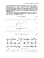
often lower than in the bulk crystal. Figure
9.9
shows the calculated trajectory of
a vacancy in the core of a large-angle tilt grain boundary in b.c.c. Fe. Calculations
showed that vacancies were more numerous and jump faster in the grain boundary
than in the crystal, indicating a vacancy mechanism for diffusion in this particular
boundary. However, there is an infinite number of different types of boundaries,
and computer simulations for other types of boundaries indicate that the dominant
mechanism in some cases may involve interstitial defects [4,
121.
During defect-mediated grain-boundary diffusion, an atom diffusing in the core
will move between the various types of sites in the core. Because various types of
jumps have different activation energies, the overall diffusion rate is not controlled

by a single activation energy. Arrhenius plots for grain-boundary diffusion therefore
should exhibit at least some curvature. However, when the available data are of only
moderate accuracy and exist over only limited temperature ranges, such curvature
may be difficult to detect. This has been the case
so
far with grain-boundary
diffusion data, and the straight-line representation of the data in the Arrhenius
Mechanism
of
Fast Grain-Boundary Diffusion
Boundary
midplane
[ooi]
Figure
9.9:
Calculated atom jumps in the core of
a
C5
symmetric
(001)
tilt boundary in
b.c.c. Fe. A
pair-potential-molecular-dynamics
model was employed. For purposes
of
clarity.
the scales used in the figure are
[I301
:
[310]

:
[OOT]
=
1
:
1
:
5.
All jumps occurred in the
fast-diffusing core region. Along the bottom, a vacancy was inserted at
B.
and subse uently
executed the series
of
jumps shown. The tra'ectory was essentially parallel to the tjt axis.
Near the center
of
the figure, an atom in a
b
site jumped into an interstitial site at
I.
At
the top an atom jumped between
B,
I
and
B'
sites.
From Balluffi
et

al.
[14].
222
CHAPTER
9
DIFFUSION ALONG CRYSTAL IMPERFECTIONS
plot in Fig. 9.3 must be regarded
as
an approximation that yields an effective
activation energy,
EB,
for the temperature range of the data. Some evidence for
curvature of Arrhenius plots for grain-boundary diffusion has been reviewed
[4].
9.3
DIFFUSION ALONG DISLOCATIONS
As with grain boundaries, dislocation-diffusion rates vary with dislocation struc-
ture, and there is some evidence that the rate is larger along a dislocation in the
edge orientation than in the screw orientation [15]. In general, dislocations in close-
packed metals relax by dissociating into partial dislocations connected by ribbons
of stacking fault as in Fig. 9.10 [16]. The degree of dissociation is controlled by
the stacking fault energy. Dislocations in A1 are essentially nondissociated because
of
its high stacking fault energy, whereas dislocations in Ag are highly dissociated
because of its low stacking fault energy. The data in Fig. 9.1 (averaged over the
available dislocation orientations) indicate that the diffusion rate along dislocations
in f.c.c. metals decreases as the degree of dislocation dissociation into partial dislo-
cations increases. This effect of dissociation on the diffusion rate may be expected
because the core material in the more relaxed partial dislocations is not as strongly
perturbed and “loosened up’’ for fast diffusion, as in perfect dislocations.

In Fig. 9.1,
*DD
for nondissociated dislocations is practically equal to
*DB,
which
indicates that the diffusion processes in nondissociated dislocation cores and large-
angle grain boundaries are probably quite similar. Evidence for this conclusion
also
comes from the observation that dislocations can support a net diffusional transport
of atoms due to self-diffusion [15]. As with grain boundaries, this supports a defect-
mediated mechanism.
The overall self-diffusion in a dislocated crystal containing dislocations through-
out its volume can be classified into the same general types of regimes
as
for a
polycrystal containing grain boundaries (see Section 9.2.1). Again, the diffusion
may be multiple
or
isolated, with
or
without diffusion in the lattice, and the dis-
locations may be stationary
or
moving. However, the critical parameters include
*DD
rather than
*DB
and the dislocation density rather than the grain size. The
multiple-diffusion regime for a dislocated crystal is analyzed in Exercise 9.1.
Figure 9.11 shows a typical diffusion penetration curve for tracer self-diffusion

into a dislocated single crystal from an instantaneous plane source at the sur-
face [17]. In the region near the surface, diffusion through the crystal directly
from the surface source is dominant. However, at depths beyond the range at
,Stacking fault
ribbon
Partial
f
2
Partial
dislocation
1
dislocation 2
Figure
9.10:
partial dislocations separated
by
a
ribbon
of
stacking fault.
Dissociated lattice dislocation in f.c.c. metal. The structure consists of two
9.4
FREE
SURFACES
223
Dislocation
pipe diffusion
C
e
Penetration depth

-w
Figure
9.11:
Typical penetration curve for tracer self-diffusion from a free surface at
tracer concentration
csurf
into a single crystal containing dislocations. Transport near the
surface is dominated by diffusion in the bulk; at greater depths, dislocation pipe diffusion is
the major transport path.
which atoms can be delivered by crystal diffusion alone, long penetrating “tails”
are present, due to fast diffusion down dislocations with some concurrent spreading
into the adjacent lattice and no overlap of the diffusion fields of adjacent dislo-
cations. This behavior corresponds to the dislocation version of the
B
regime in
Fig.
9.4.
9.4
DIFFUSION ALONG FREE SURFACES
The general macroscopic features of fast diffusion along free surfaces have many
of the same features as diffusion along grain boundaries because the fast-diffusion
path is again a thin slab of high diffusivity, and
a
diffusing species can diffuse in
both the surface slab and the crystal and enter or leave either region. For example,
if a given species is diffusing rapidly along the surface,
it
may leak into the adjoining
crystal just as during type-B kinetics for diffusion along grain boundaries. In fact,
the mathematical treatments of this phenomenon in the two cases are similar.

The structure
of
crystalline surfaces is described briefly in Sections
9.1
and
12.2.1
and in Appendix B. All surfaces have a tendency to undergo a “roughening” tran-
sition at elevated temperatures and
so
become general. Even though a considerable
effort has been made, many aspects of the atomistic details of surface diffusion are
still unknowns6
For singular and vicinal surfaces at relatively low temperatures, surface-defect-
mediated mechanisms involving single jumps of adatoms and surface vacancies are
pred~minant.~ Calculations indicate that the formation energies of these defects
are of roughly comparable magnitude and depend upon the surface inclination [i.e.,
(hkl)].
Energies of migration on the surface have also been calculated, and in
most cases, the adatom moves with more difficulty. Also, as might be expected,
the diffusion on most surfaces is anisotropic because of their low two-dimensional
symmetry. When the surface structure consists
of
parallel rows of closely spaced
atoms, separated by somewhat larger inter-row distances, diffusion is usually easier
parallel to the dense rows than across them. In some cases,
it
appears that the
60ur
discussion follows reviews
by

of Shewmon
[18]
and Bocquet et al.
[19].
7Adatoms, surface vacancies, and other features of surface structure are depicted in Fig.
12.1
224
CHAPTER
9:
DIFFUSION
ALONG
CRYSTAL
IMPERFECTIONS
transverse diffusion occurs by a replacement mechanism in which an atom lying
between dense rows diffuses across a row by replacing an atom in the row and
pushing the displaced atom into the next valley between dense rows. Repetition of
this process results in a mechanism that resembles the bulk interstitialcy mechanism
described in Section
8.1.3.
In addition, for vicinal surfaces, diffusion rates along
and over ledges differs from those in the nearby singular regions.
At more elevated temperatures, the diffusion mechanisms become more complex
and jumps to more distant sites occur, as do collective jumps via multiple defects.
At still higher temperatures, adatoms apparently become delocalized and spend
significant fractions of their time in “flight” rather than in normal localized states.
In many cases, the Arrhenius plot becomes curved at these temperatures (as in
Fig.
9.1),
due
to

the onset
of
these new mechanisms. Also, the diffusion becomes
more isotropic and less dependent on the surface orientation.
The mechanisms above allow rapid diffusional transport of atoms along the sur-
face. We discuss the role of surface diffusion in the morphological evolution of
surfaces and pores during sintering in Chapters
14 and
16,
respectively.
Bibliography
1.
N.A. Gjostein. Short circuit diffusion. In
Diffusion,
pages 241-274. American Society
for Metals, Metals Park, OH, 1973.
2. I. Herbeuval and M. Biscondi. Diffusion of zinc in grains of symmetric flexion
of
aluminum.
Can. Metall. Quart.,
13(1):171-175, 1974.
Diffusion in ceramics. In R.W. Cahn,
P.
Haasen, and
E.
Kramer,
editors,
Materials Science and Technology-A Comprehensive Treatment,
volume
11,

pages 295-337, Wienheim, Germany, 1994. VCH Publishers.
4. A.P. Sutton and R.W. Balluffi.
Interfaces
in
Crystalline Materials.
Oxford University
Press, Oxford, 1996.
5. E.W. Hart.
On the role of dislocations in bulk diffusion.
Acta Metall.,
5(10):597,
1957.
6.
L.G. Harrison. Influence of dislocations on diffusion kinetics in solids with particular
reference to the alkali halides.
Trans. Faraday Soc.,
57(7):1191-1199, 1961.
7.
D.
Turnbull. Grain boundary and surface diffusion. In J.H. Holloman, editor,
Atom
Movements,
pages 129-151, Cleveland,
OH,
1951.
American Society
for
Metals. Spe-
cial Volume
of ASM.

8. J.W. Cahn and R.W. Balluffi. Diffusional mass-transport in polycrystals containing
stationary
or
migrating grain boundaries.
Scripta Metall. Mater.,
13(6):499-502, 1979.
9. I. Kaur and W. Gust.
Fundamentals of Grain and Interphase Boundary Diffusion.
Ziegler Press, Stuttgart, 1989.
10.
J.C. Fisher. Calculation of diffusion penetration curves for surface and grain boundary
diffusion.
J.
Appl. Phys.,
22(1):74-77, 1951.
11.
J.C.M. Hwang and R.W. Balluffi. Measurement of grain-boundary diffusion at low-
temperatures by the surface accumulation method
1.
Method and analysis.
J.
Appl.
12.
Q.
Ma and R.W. Balluffi. Diffusion along
[OOl]
tilt boundaries in the Au/Ag system
1.
Experimental results.
Acta Metall.,

41(1):133-141, 1993.
13.
R.W. Balluffi. Grain boundary diffusion mechanisms in metals. In G.E. Murch and
AS.
Nowick, editors,
Diffusion
in
Crystalline Solids,
pages 319-377, Orlando, FL,
1984. Academic Press.
3.
A. Atkinson.
Phys.,
50(3):1339-1348, 1979.
EXERCISES
225
14.
R.W. Balluffi,
T.
Kwok, P.D. Bristowe, A. Brokman, P.S.
Ho,
and
S.
Yip. Deter-
mination of the vacancy mechanism for grain-boundary self-diffusion by computer
simulation.
Scripta
Metall.
Mater.,
15(8):951-956, 1981.

On measurements of self diffusion rates along dislocations in f.c.c.
metals.
Phys. Status Solidi,
42(1):11-34, 1970.
16.
R.E. Reed-Hill and R. Abbaschian.
Physical Metallurgy Principles.
PWS-Kent,
Boston,
1992.
17.
Y.K.
Ho and P.L. Pratt. Dislocation pipe diffusion in sodium chloride crystals.
Radiat.
18.
P.
Shewmon.
Diffusion
in
Solids.
The Minerals, Metals and Materials Society, War-
rendale, PA,
1989.
19.
J.L.
Bocquet,
G.
Brebec, and Y. Limoge.
Diffusion in metals and alloys. In R.W.
Cahn and

P.
Haasen, editors,
Physical Metallurgy,
pages
535-668.
North-Holland,
Amsterdam, 2nd edition,
1996.
15.
R.W.
Balluffi.
Eff.,
75~183-192, 1983.
EXERCISES
9.1
In a Type-A regime, short-circuit grain-boundary self-diffusion can enhance
the effective bulk self-diffusivity according to Eq. 9.4. A density of lattice
dislocations distributed throughout a bulk single crystal can have a similar
effect if the crystal diffusion distance for the diffusing atoms is large compared
with the dislocation spacing.
Derive an equation similar
to
Eq. 9.4 for the effective bulk self-diffusivity,
(*D),
in the presence of fast dislocation diffusion. Assume that the dislocations are
present at a density,
p,
corresponding to the dislocation line length in a unit
volume
of

material.
Solution.
During self-diffusion, the fraction of the time that a diffusing atom spends
in dislocation cores is equal to the fraction of all available sites that are located in
the dislocation cores.
This fraction will be
7
=
p7d2/4.
The mean-square displace-
ment due to self-diffusion along the dislocations is then
*DDqt,
while the corresponding
displacement in the crystal is
*DxL(l
-
7)t.
Therefore,
(*D)t
=
*DXL(l
-
7)t
+
*DD7t
(9.17)
and because
7
<<
1,

(9.18)
p7rP
(*D)
=
*DxL
+
-
*DD
4
9.2
Exercise 9.1 yielded an expression, Eq. 9.18, for the enhancement
of
the ef-
fective bulk self-diffusivity due to fast self-diffusion along dislocations present
in the material at the density,
p.
Find a corresponding expression for the
enhancement of the effective bulk self-diffusivity of solute atoms due to
fast
solute self-diffusion along dislocations. Assume that the solute atoms segre-
gate to the dislocations according
to
simple McLean-type segregation where
cf/cf"
=
k
=
constant, where
cf
is the solute concentration in the disloca-

tion cores and
cfL
is the solute concentration in the crystal.
Solution.
Because the fraction of solute sites in the dislocations is small, the number
of occupied solute-atom sites (per unit volume) in the crystal is
cgL,
and the number of
226
CHAPTER
9:
DIFFUSION
ALONG
CRYSTAL
IMPERFECTIONS
occupied sites in the dislocations is
pd2kc?XL/4.
The fraction of time that a diffusing
solute atom spends in dislocation cores is then
17
=
p7d2k/4.
Therefore, following the
same argument as in Exercise
9.1,
(*Dz)t
=
*D,””(l
-
v)t

+
*Dpqt (9.19)
and thus
(*D2)
=
*DfL
+
@
*Df
(9.20)
4
9.3
For Type-B diffusion along a grain boundary, Eq. 9.9, which holds for self-
diffusion, takes the form of Eq. 9.15 for solute diffusion when simple McLean-
type segregation occurs with
cf/cgL
=
k.
Show that this causes Eq. 9.13,
which holds for self-diffusion, to take the form
(9.21)
for solute diffusion.
Solution.
As
indicated in the text, Eq.
9.9
must have the form of Eq.
9.15
in order
to satisfy the segregation condition

k
=
cf/c?”
at the boundary slab. Equation
9.10
then becomes
Equation
9.11
becomes
[
-
(A)
Yl]
B
c2
(yi,ti)
=
exp
(9.23)
Equation
9.12
becomes
cz
XL
(zl,yl,tl)
=
-exp
1
[-
(A)”*

YI]
[1
-erf
-$)I
(9.24)
k
and, finally, Eq.
9.13
becomes
(9.25)
9.4
As
described in Section 9.2.2, grain-boundary diffusion rates in the Type-C
diffusion regime can be measured by the surface-accumulation method illus-
trated in Fig. 9.12. Assume that the surface diffusion is much faster than the
grain-boundary diffusion and that the rate at which atoms diffuse from the
%ource” surface to the “accumulation” surface is controlled by the diffusion
rate along the transverse boundaries. If the diffusant, designated component
2,
is initially present on the source surface and absent on the accumulation
surface and the specimen is isothermally diffused, a quasi-steady rate of ac-
cumulation of the diffusant is observed on the accumulation surface after a
short initial transient. Derive a relationship between the rate of accumulation
EXERCISES
227
and the parameter
SDF
that can be used to determine
SDf
experimentally.

Assume that each grain is a square of side
d
in the plane of the surface.
c
Source
surface
Fil
thi
Accumulation surface
Figure
9.12:
diffusion.
Transport
of
diffusant
through
a thin polycrystalline film
by
grain-boundary
Solution.
Because of the fast surface diffusion, the concentrations of the diffusant
on both surfaces are essentially uniform over their areas. After the initial transient, the
quasi-steady rate (per unit area of surface)
at
which the diffusant diffuses along the
transverse boundaries between the two surfaces is
Here,
d
is the average grain size of the columnar grains,
JB

is the diffusional flux
along the grain boundaries,
dcB/dx
=
[cB(0)
-
cB(I)]
/I,
where
cB(0)
and
cB(I)
are
the diffusant concentrations in the boundaries at the source surface and accumulation
surface, respectively, and
I
is the specimen thickness. In the early stages,
cB(I)
=
0
and, therefore, to a good approximation,
B
Id
dN
6D2
=
-
-
2cB(0)
dt

(9.27)
All quantities on the right-hand side of Eq.
9.27
are measurable, which allows the
determination of
bDf
[12].
9.5
Using the result of Exercise 9.1 and data in Fig. 9.1, estimate the density
of
dissociated dislocations necessary to enhance the average bulk self-diffusivity
by a factor of 2 at
Tm/2,
where
T,
is the absolute melting temperature of the
material.
Note:
typical dislocation densities in annealed f.c.c. metal crystals
are in the range 106-108
cm-2.
Solution.
Equation
9.18
may be solved for
p
in the form
(9.28)
It
is estimated from Fig.

9.1
that
*DD(dissoc)/*DXL
=
3
x
lo6
at
Tm/T
=
2.0.
Also,
6
%
6
x
lo-*
cm-*. Using these values and
(*D)/*DxL
=
2
in Eq.
9.28,
p
E
10'
cmP2
Therefore,
it
appears that the dislocations could make a significant contribution to

diffusion under many common conditions.
228
CHAPTER
9:
DIFFUSION
ALONG
CRYSTAL IMPERFECTIONS
9.6
The asymmetric small-angle tilt boundary in Fig.
B.5a
consists of an array
of parallel edge dislocations running parallel to the tilt axis. During diffusion
they will act as fast diffusion “pipes.” Show that fast self-diffusion along this
boundary parallel to the tilt axis can be described by an overall boundary
diffusivity,
e
(9.29)
lr
4
where
b
is the magnitude of the Burgers vector and
6’
is the tilt angle.
sin
4
+
cos
4
b

*DB(para)
=
-
*DD6
Use
*DD
>>
*DL
(9.30)
Solution.
As
usual, take the boundary as a slab that is
6
thick. In considering diffusion
along the tilt axis, any contribution of the crystal regions in the slab can be neglected
and only the contributions of the dislocation pipes are included because
*DD
>>
*DxL.
The flux through a unit cross-sectional area of the boundary slab
is
then
(9.31)
where the first bracketed term is the flux along
a
single pipe and the second
is
the
number of pipes per unit area of the boundary slab. The desired expression
is

obtained
by equating this result with
J
=
-
*DB(para)
&/ax
and solving for
*DB.
9.7
Self-diffusion along the boundary in Exercise
9.6
is highly anisotropic because
diffusion along the tilt axis (parallel to the dislocations) is much greater than
diffusion transverse to it (i.e., perpendicular to the dislocations but still in
the boundary plane). Find an expression for the anisotropy factor,
*D
(para)
*D (transv)
(9.32)
where *DB (transv) is the boundary diffusivity in the transverse direction.
Solution.
The transverse diffusion rate is controlled by the relatively slow crystal
diffusion rate because the diffusing atoms must traverse the patches of perfect crystal
between the dislocation pipes. Therefore, when the dislocations are discretely spaced,
a good approximation is the simple result
*DB
(para)
-
*DB (para)

-
*DB(transv) *DxL
(9.33)
CHAPTER
10
DIFFUSION IN NONCRYSTALLINE
M
AT
E
R
I
A LS
Noncrystalline materials exist in many different forms.
A
huge variety of atomic
and molecular structures, ranging from liquids to simple monatomic amorphous
structures to network glasses to dense long-chain polymers, are often complex and
difficult to describe. Diffusion in such materials occurs by a correspondingly wide
variety of mechanisms, and is, in general, considerably more difficult to analyze
quantitatively than is diffusion in crystals.
The understanding of diffusion in many noncrystalline materials has lagged be-
hind the understanding of diffusion in crystalline material, and a unified treatment
of
diffusion in noncrystalline materials is impossible because of its wide range of
mechanisms and phenomena. In many cases: basic mechanisms are still controver-
sial or even unknown. We therefore focus on selected cases, although some of the
models discussed are still under development and not yet firmly established.
10.1
FREE-VOLUME MODEL FOR SELF-DIFFUSION IN LIQUIDS
Self-diffusion in simple monatomic liquids at temperatures well above their glass-

transition temperatures may be interpreted in a simple manner.' Within such
liquids, regions with
free
volume
appear due to displacement fluctuations. Occa-
sionally, the fluctuations are large enough to permit diffusive displacements.
'This section closely follows Cohen and Turnbull's original derivation
[l].
The original paper
should be consulted for further details.
Kinetics
of
Materials.
By Robert
W.
Balluffi, Samuel
M.
Allen, and
W.
Craig Carter.
229
Copyright
@
2005 John Wiley
&
Sons, Inc.
230
CHAPTER
10:
DIFFUSION

IN
NONCRYSTALLINE
MATERIALS
The
hard-sphere
model
for the liquid serves as a reasonably good approximation
for the atomic interactions [2]. Here, the potential energy between any pair of
approaching particles is assumed to be constant until they touch, at which point it
becomes infinite. On average, the particles in the liquid maintain a volume larger
than that which they would have if they all touched; the resulting volume difference
is the free volume. Each particle effectively traverses a small confined volume within
which the interatomic potentials are essentially flat [3]. The average velocity
of
a
particle in the region of flat potential inside the confining volume is the same as
the velocity of a gas particle. Most .of the time a particular particle is confined
to a particular region. However, there will occasionally be a fluctuation in local
density that opens a space large enough to permit a considerable displacement of the
particle. If another particle jumps into that space before the displaced first particle
returns, a diffusive-type jump will have occurred. Diffusion therefore occurs as a
result of the redistribution of the free volume that occurs at essentially constant
energy because of the flatness of the interatomic potentials.
According to the kinetic theory of gases, the self-diffusivity of a hard-sphere
gas is given by
*DG
=
(2/5)(u)L, where
(u)
is the average velocity and

L
is
the
mean free path
[4].
Because the mean free path of a confined particle in the liquid is
about equal
to
the diameter of its confining volume, the contribution of the confined
particle to the self-diffusivity of the liquid may be written
’
*D(V)
=
Cgeom
a(V)
(u)
(10.1)
where
u(V)
is the diameter of the confining volume,
V
is the free volume associ-
ated with the particle,
(u)
is the average velocity of the particle, and
C,,,,
is a
geometrical constant.It is reasonable to assume that the diffusivity is very small,
*D(V)
=

0,
unless the local free volume
V
exceeds a critical volume,
Vcrit.
There-
fore, the overall diffusivity may be expressed
(10.2)
where
p(V) dV
is the free volume’s probability that it lies between
V
and
V
+
dV.
To determine this probability distribution, consider a system containing
n/
particles
and divide the total range of possible free volumes for a particle into bins indexed
by
i.
Let
Ni(V,)
be the number of particles with free volume
V,.
If
Vfree
is the total
free volume, the condition

Vfree
=
NiV,
(10.3)
i
must hold. The factor
y
accounts for all free-volume overlap between adjacent
particles.
y
lies between zero and one because of the physical limits of complete
and no overlap; its value is probably closer to one. The total number of particles,
N.
is
(10.4)
i
The entropy associated with the number of ways that the free volume can be
distributed at constant energy is
(10.5)