Kinetics of Materials - R. Balluff_ S. Allen_ W. Carter (Wiley_ 2005) Episode 14 pps

574
CHAPTER
24:
MARTENSITIC TRANSFORMATIONS
When the shape change is relatively large, the parent phase will no longer be
able to accommodate the inclusion elastically, and anticoherency lattice dislocations
will be generated to relieve the long-range stress field and reduce the elastic energy.
Plastic deformation will therefore occur in the parent phase, and anticoherency
dislocations will be added to the interface. These dislocations will generally tend
to reduce the mobility of the interface.
Because martensite interfaces can be represented as arrays of dislocations, the
velocity with which they move will generally be controlled by the same factors that
control the rate of glide motion of crystal dislocations. As discussed in Section 11.3,
these include dissipative drag due to phonons and free electrons and interactions
with a large variety of different types of crystal imperfections which hinder their
glide motion. When the martensite forms as enclosed platelets
as
in Fig. 24.12,
additional work must also be done to produce the increase in interfacial area that
occurs
as
the platelets grow. An extensive discussion of the factors involved in
the motion of martensite interfaces has been given by Olson and Cohen [9]. As
pointed out in Section 11.3.4, there is no clear evidence for the supersonic motion
of martensite interfaces. However, velocities on the order of the speed of sound can
be achieved in the presence of large driving forces.
24.4
NUCLEATION
OF
MARTENSITE
The homogeneous nucleation of martensite in typical solids is too slow by many

orders of magnitude to account for observed results. Calculations of typical values
of
AGc
using the classical nucleation model of Section 19.1.4 (see Exercise 19.3) yield
values greatly exceeding
76
kT.
Furthermore, nearly all martensitic transformations
commence at very sparsely distributed sites.
Small-particle experiments
[14] have
yielded typical nucleation densities on the order of one nucleation event per
50
pm
diameter Fe-Ni alloy powder parti~le.~ Thus, nucleation of martensite is believed
to occur
at
a
small number of especially potent heterogeneous nucleation sites.
The most likely special site for martensitic nucleation is
a
pre-existing dislocation
array, such as a portion of a tilt boundary [9]. The nucleation process involves dis-
sociation of the boundary dislocations,
so
as
to produce periodic faults in the parent
crystal and thereby provide a mechanism for the lattice deformation. The process
of superimposing lattice-invariant deformation onto the deformation that occurs in
the dissociation of the original tilt boundary is used to obtain the equivalent of the

lattice deformation
RB
in the crystallographic model of Section 24.2.4. The rate of
initiating such a nucleus is limited by the rate at which the dislocations required to
form and then expand the configuration can move under the available driving force.
The entire process may be free of any energy barrier under sufficiently high driving
forces, or else involve local barriers to certain critical dislocation movements which
can be surmounted with the assistance of thermal activation. Details of the specific
defects required for the mechanism have been worked out for common structural
changes (e.g., f.c.c.+ h.c.p., f.c.c.+ b.c.c.)
[8,
91.
3Small-particle experiments are carried out by studying nucleation in small particles of the parent
phase and are useful in distinguishing between homogeneous and heterogeneous nucleation. If
the nucleation is homogeneous, the nucleation rate is simply proportional to the volume
of
the
particle. On the other hand, if it is heterogeneous, the rate goes essentially to zero when the
particle size is lower than
l/p,
where
p
is the density of heterogeneous nucleation sites.
24
5:
EXAMPLES
OF
MARTENSITIC
TRANSFORMATIONS
575

24.5
MARTENSITIC TRANSFORMATIONS IN THREE CONTRASTING
SYSTEMS
We now describe briefly martensitic transformations in three contrasting systems
which illustrate some of the main features of this type of transformation and the
range of behavior that is found [15]. The first is the In-T1 system, where the lattice
deformation is relatively slight and the shape change is small. The second is the
Fe-Ni system, where the lattice deformation and shape change are considerably
larger. The third is the FeNi-C system, where the martensitic phase that forms
is metastable and undergoes a precipitation transformation
if
heated.
24.5.1 In-TI
System
Upon cooling, an In-T1 (19%
T1)
alloy undergoes an f.c.c. solid solution
+
f.c.t. solid
solution martensitic transformation in which the lattice deformation is relatively
slight, corresponding to
(24.9)
0
1.0238
OI
0.9881
0
B
=
[Bij]

=
0
0.9881
0
[o
and the shape change is correspondingly small. The lattice-invariant deformation is
accomplished by means of twinning in this system,
so
the low-temperature marten-
sitic phase consists of twin-related lamellae. If a rod-shaped single crystal of the
parent f.c.c. phase is carefully cooled in a small temperature gradient from above
the transformation temperature, the transformation can be induced
so
that the
martensite first appears at the cooler end of the specimen as
a
region separated
from the parent phase by a single planar interface that spans the entire cross sec-
tion of the specimen.
As
cooling continues, the single interface advances along the
rod until the entire specimen is transformed. Upon subsequent reverse heating, the
transformation is found to be reversible and the original single crystal of the parent
phase is recovered with a temperature hysteresis of only about 2",
as
shown in
Fig. 24.13, where the progress of the transformation is indicated by measurements
of the length change of the specimen.
L'
' '

I'
'
'
I'
'J
w66
68
70
72
74 76
Temperature
("C)
Figure
24.13:
Temperature dependence of the martensitic transformation in In-20.7
at.
%
T1. The extent of transformation is revealed
by
changes of specimen len th caused
by the transformation. The dashed line shows the reversible transformation res5ting from
continuous cooling and heating. The solid line shows stabilization of the transformation
induced during the heating part of the cycle by a hold of
6
h at constant temperature.
From
Burkart
and
Read
[16].

576
CHAPTER
24:
MARTENSITIC TRANSFORMATIONS
f.c.c.
0.2
01
'
'
'
' ' ' ' '
'
'
'1
66
68
I0
12
14
16
Temperature
("C)
Figure
24.14:
Temperature dependence of martensitic transformation in In-20.7 at.
'%
T1 under
two
different com ressive stresses. Phase fraction of martensite
is

proportional to
the permanent strain whicl? can be determined by the stress-free specimen length.
From
Burkae and Read
[16].
The interface motion is jerky on a fine scale and requires a continuous drop in
temperature. This indicates that the interface requires a continuous increase in
driving pressure (brought about by increased undercooling) to maintain its motion.
This may be taken as evidence that the interface must be accumulating defects due
to interactions with obstacles in its path which progressively reduce its mobility.
If the heating (or cooling) is interrupted by a hold at constant temperature, the
interface becomes stabilized as shown in Fig. 24.13. During the holding period, no
further transformation occurs, and then a jump in temperature is required to restart
the transformation. This is apparently due to an unidentified time-dependent re-
laxation
at
the interface that occurs during the hold. The extent of transformation
therefore depends primarily on the temperature and not on time. The transfor-
mation is therefore considered to be
athermal
to distinguish it from an
isothermal
transformation, which progresses with increasing time at constant temperature.
The transformation can be influenced by an applied stress.
As
seen in Fig. 24.13,
the stress-free transformation to martensite results in a decrease in specimen length.
Data in Figs. 24.14 and 24.15 were obtained by applying a series
of
constant uniax-

ial stresses at constant ambient pressure,
P.
The data show that the transforma-
tion temperature increases approximately linearly with applied uniaxial compressive
stress. This dependence of transformation temperature on stress state follows from
minimization of the appropriate thermodynamic function. For a material under
I-
60-
0 0.1 0.2
0.3
Compressive stress
(MPa)
Figure
24.15:
of applied compressive stress.
Martensite transformation temperature in In-20.7
at.
%
T1
as
a function
From Burkart and Read
[16].
24.5:
EXAMPLES OF MARTENSITIC TRANSFORMATIONS
577
uniaxial stress, this function takes the form
Guni
=
Uuni

-
TS
+
p
v
-
v,
,+p,uni(l
+
pas,uni
1
(24.10)
where
Uuni
is the reversible adiabatic work to take a system from a reference state
to a state of uniaxial
m tress.^
aapp,uni
is the applied uniaxial stress above the
gauge
hydrostatic stress,
-P,
and
E~'~~+~~
is the
elastic
strain in the axial direction.
V,
is
a reference molar volume, which can be taken to be the molar volume of the parent

phase at one atmosphere (i.e.'
V,
=
Vpar).
Let the uniaxial strain associated with the martensite transformation be
SE;$~,
Emeas,uni
.
The
and parent phases, respectively. It is not necessary that
EEF'~~~
=
par
elastic parts of the uniaxial strains in the two phases will be related through their
respective elastic constants because the normal components of stress must be equal
at
the interface.
The differential forms of the molar free energy for the parent and martensite
phases are
and let
pF,uni
and
pas,uni
par
be the
measured
uniaxial strains in the martensite
meas,uni
dGEdrt
=

-
Smart
dT
+
Vmart
dP
-
Vo(l
+
emart
-
&girt)
dc7app3uni
(24.11)
This analysis shows that a compressive load decreases the molar free energy-
and that a positive
&:$,
reduces the magnitude of the decrease for the marten-
site phase thereby resulting in an increased transformation temperature, consistent
with Fig. 24.16. Further analysis shows that the observed shift in transformation
temperature results from differences in the Young's moduli of the two phases (see
Exercise
24.5).
This result is consistent with LeChatelier's principle.
dG:i?
=
-
Spar
dT
+

Vpar
dP
-
V,
(1
+
E~~~'~~~)
daaPP,uni
t
s
F
C
Figure
24.16:
Free energy of parent and martensite phases
as
a function of temperature,
illustrating the effect
of
compressive uniaxial stress on martensite transformation
temperature in In-T1 crystals.
4U
has the differential
dU""'
=
T
dS
-
P
dV

+
VouaPP,uni
dcelas~uni.
Considering that this energy
change must reduce to the fluidlike
P
dV
work
under pure hydrostatic loading, the
(1
+
cii)-terms
must appear because
CE.~
=
AV/Vo
=
V/Vo
-
1.
578
CHAPTER
24:
MARTENSITIC TRANSFORMATIONS
Further work found that the transformation in In-TI alloys could be induced
isothermally (i.e., without any cooling whatsoever) by the application and removal
of a sufficiently large compressive load
[16].
This is consistent with the data in
Fig.

24.15,
which show that there are conditions where the transformation temper-
ature on cooling of the stressed specimen is above the transformation temperature
of the unstressed specimen on heating,
as
would be required.
24.5.2
Fe-Ni
System
Upon cooling, an Fe-Ni
(29.3
wt.
%
Ni) alloy undergoes an f.c.c. solid solution
+
b.c.c. solid solution martensitic transformation in which the lattice deformation is
an order of magnitude larger than in the In-T1 transformation and is
B
=
[Bij]
=
0
1.13
0
(24.12)
[
l:
1
010
1

The transformation is again found to be reversible and to exhibit hysteresis as
shown in Fig.
24.17,
which shows
a
cooling and heating cycle, detected by means
of electrical resistivity measurements. However, the hysteresis, corresponding to
about
450°C,
is much larger than in the In-T1 system, indicating that a much larger
pressure is required to drive the transformation. Examination of the morphology
of the transformation shows that
it
is quite different than in the In-T1 case. The
martensite now forms as small lenticular platelets embedded in the parent phase,
with their habit planes parallel to variants of the invariant plane,
as
shown in
Fig.
24.18.
The manner in which the transformation progresses during cooling is
also quite different. After forming, each platelet grows very rapidly to a final size
and then remains static. As cooling continues, the transformation then progresses
by the formation of new platelets. This behavior is attributed to the large lattice
deformation, causing a large shape change in this system, which is too large to be
accommodated elastically. Instead, plastic flow occurs in the parent phase in the
form
of
the generation and movement of dislocations, and anticoherency dislocations
are introduced in the platelet interfaces, causing them to lose their mobility as

described in Section
24.3.
This explanation
is
consistent with the large amount of
hysteresis observed upon thermal cycling, since this reduction of mobility makes
it
difficult to reverse the direction of motion of the platelet interfaces.
2.0
G
1.6
-
1.2
-
8
s
0.8
c
v)

0.4
lx
-100
0
100
200
300
400
500
Temperature

("C)
Figure
24.17:
Temperature dependence of the martensitic transformation in the Fe-Ni
(29.3
wt.
%)
system during thermal cycle. Extent of transformation revealed by change of
specimen electrical resistivity.
From Kaufman and Cohen
[17].
24.5:
EXAMPLES OF MARTENSITIC TRANSFORMATIONS
579
Figure
24.18:
Fe-32
wt.
%
Ni alloy.
From
the
ASM
Metals
Handbook,
Vol.
8,
p.
198.
Martensite platelets formed in the f.c.c.

-+
b.c.c. transformation in an
The phenomenon of stabilization is also observed in this system if the cooling
is interrupted and the specimen is held isothermally before cooling is resumed.
In this case, the transformation resumes only after the driving force is incremen-
tally increased by
a
significant drop in temperature. Again, the transformation is
primarily athermal, depending upon decreases of temperature which provide corre-
sponding increases in the driving pressure for the formation of more platelets. Also,
a
relatively small amount of isothermal formation of martensite is observed if the
specimen is rapidly quenched into the temperature range where martensite forms
and is then held isothermally
[18].
However, the isothermal transformation occurs
by the formation of new platelets and not by the growth of existing ones.
In general, the result that the platelets form very rapidly (at speeds of the order
of the speed of sound)
at
relatively low temperatures,
at
rates that are not signifi-
cantly temperature-dependent, indicates that the platelet growth is not thermally-
activated and occurs only when a sufficiently high driving pressure is available.
24.5.3 Fe-Ni-C
System
The crystallography of the f.c.c + b.c.t. martensitic transformation in the Fe-Ni-C
system (with
22

wt. %Ni and
0.8
wt. %C) has been described in Section
24.2.
In
this system, the high-temperature f.c.c. solid-solution parent phase transforms upon
cooling to a b.c.t. martensite rather than
a
b.c.c. martensite
as
in the Fe-Ni system.
Furthermore, this transformation is achieved only if the f.c.c. parent phase is rapidly
quenched. The difference in behavior is due to the presence of the carbon in the
Fe-
Ni-C alloy. In the Fe-Ni alloy, the b.c.c. martensite that forms
as
the temperature
is lowered is the equilibrium state of the system. However, in the Fe-Ni-C alloy, the
equilibrium state of the system in the low-temperature range is
a
two-phase mixture
of
a
b.c.c. Fe-Ni-C solid solution and
a
C-rich carbide phase.5 This difference in be-
havior is due to a much lower solubility of C in the low-temperature b.c.c. Fe-Ni-C
phase than in the high-temperature f.c.c. Fe-Ni-C phase. If the high-temperature
5The true equilibrium state is the FeNi-C phase plus graphite. However, the carbide phase is
so

strongly metastable that it
can
be regarded
as
an
“equilibrium” phase.
580
CHAPTER
24.
MARTENSITIC TRANSFORMATIONS
f.c.c. Fe-Ni-C parent phase were to be slowly cooled under quasi-equilibrium condi-
tions, it would undergo diffusional phase changes resulting in the ultimate formation
of the two-phase mixture. However, if the parent phase is rapidly quenched, these
phase changes are bypassed and it transforms martensitically to the solid-solution
b.c.t. phase, which is therefore a nonequilibrium phase that is metastable to the
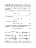
formation of the equilibrium two-phase mixture. During the quench, the
C
atoms
are trapped in the interstitial positions they occupied in the parent phase,
as
shown
in Fig.
24.3.
By comparing these positions with Fig.
8.8a,
it may be seen that they
are
a
subset of the complete set of lattice-equivalent interstitial sites that carbon
atoms can occupy in the b.c.c. structure.6 Carbon atoms occupying interstitial sites

generally act as positive centers of dilation that push most strongly against their
nearest-neighbors. The carbon atoms that randomly occupy the sites in Fig.
24.3
push most strongly along the
z
axis and
so
produce the observed tetragonality. The
b.c.t. phase can be considered as a b.c.c. structure that has been forced into tetrag-
onality by quenched-in C atoms that occupy positions inherited from the parent
f.c.c. phase.
Once the system is cooled to a low enough temperature to preclude any carbide
formation due to diffusion, further martensite can be produced by further drops
in temperature. The overall transformation on cooling then has many of the fea-
tures of the transformation in the FeNi alloy described above. The shape change
is large, the martensite forms
as
embedded lenticular platelets, and the formation
is athermal and requires continuously decreasing temperatures to proceed signifi-
cantly. However, the transformation is not reversible
as
in theFe-Ni system. When
the Fe-Ni-C martensite is heated, it decomposes by precipitating the more stable
carbide phase before it is able to transform back to the high-temperature f.c.c.
parent phase.
This behavior is typical of steels that are alloys composed mainly of iron and car-
bon and, in many cases, additional alloying elements such
as
nickel, chromium, or
manganese. The martensite formed directly after quenching is exceedingly hard but

quite brittle. However, it can then be toughened by subsequent heating (temper-
ing), which allows some controlled carbide precipitation. Extraordinary mechanical
properties can be obtained by this combination
of quenching and tempering, and
it forms the basis for the heat treatment of steel
[15].
Bibliography
1.
W.S. Wechsler,
D.S.
Lieberman, and
T.A.
Read. On the theory of the formation of
martensite.
Trans. AIME,
197( 11):1503-1515, 1953.
2.
J.S. Bowles and J.K. MacKenzie. The crystallography of martensite transformations
I.
Acta Metall.,
2(1):129-137, 1954.
3.
J.S. Bowles and J.K. MacKenzie. The crystallography of martensite transformations
11.
Acta Metall.,
2(1):138-147, 1954.
4.
J.S. Bowles and J.K. MacKenzie. The crystallography of martensite transformations.
111.
Face-centered cubic

to
body-centered tetragonal transformations.
Acta Metall.,
5.
C.M.
Wayman.
Introduction
to
the Crystallography
of
Martensitic Ransformations.
2(2):224-234, 1954.
Macmillan, New
York,
1964.
6Note that the number
of
carbon atoms occupying these sites
is
considerably smaller than the
number
of
sites and that the sites are therefore sparsely populated.
EXERCISES
581
6. J.W. Christian. Martensitic transformations. In R.W. Cahn, editor,
Physical Metal-
lurgy,
pages 552-587. North-Holland, New York, 1970.
7. M. Cohen and C.M. Wayman. Fundamentals of martensitic reactions. In J.K. Tien

and J.F. Elliott, editors,
Metallurgical Treatises,
pages 455-468. The Metallurgical
Society of AIME, Warrendale, PA, 1981.
8.
G.B. Olson and M. Cohen. Theory of martensitic nucleation: A current assessment. In
Proceedings
of
an International Conference on Solid+Solid Phase Transformations,
pages 1145-1164, Warrendale, PA, 1982. The Metallurgical Society of AIME.
9. G.B. Olson and M. Cohen. Dislocation theory of martensitic transformations. In
F.R.N. Nabarro, editor,
Dislocations in Solids,
Vol.
7,
pages 295-407. North-Holland,
New York, 1986.
10. C.S. Barrett and T.B. Massalski.
Structure
of
Metals: Crystallographic Methods,
11.
J.M. Ball and R.D. James. Fine phase mixtures
as
minimizers of energy.
Arch. Rat.
12. J.M. Ball. The calculus of variations and materials science.
Quart. Appl. Math.,
13. J.M. Ball and R.D. James. Theory for the microstructure of martensite and applica-
tions. In

Proceedings
of
the International Conference on Martensitic Transformations,
pages 65-76, Monterey, CA, 1993. Monterey Institute for Advanced Studies.
14. R.E. Cech and D. Turnbull. Heterogeneous nucleation of the martensite transforma-
tion.
Trans. AIME,
206:124-132, 1956.
15. R.E. Reed-Hill and R. Abbaschian.
Physical Metallurgy Principles.
PWS-Kent,
Boston, 1992.
16. M.W. Burkart and T.A. Read. Diffusionless phase change in the indium-thallium
system.
Trans. AIME,
197:1516-1524, 1953.
17.
L.
Kaufman and M. Cohen. The martensitic transformation in the iron-nickel system.
Trans. AIME,
206:1393-1400, 1956.
18. E.S. Machlin and M. Cohen. Isothermal mode of the martensitic transformation.
Trans. AIME,
194:489-500, 1952.
deformation.
Acta Metall.,
6:680-693, 1958.
Principles and Data.
Pergamon Press, New York,
3rd

edition, 1980.
Mech. Anal.,
100:13-52, 1987.
56( 4)
:
719-740, 1998.
19.
D.S.
Lieberman. Martensitic transformations and determination of the inhomogeneous
20.
J.F.
Nye.
Physical Properties
of
Crystals.
Oxford University Press, Oxford, 1985.
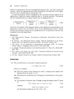
EXERCISES
24.1
It has been stated that “a martensitic phase transformation can be considered
as
the spontaneous plastic deformation of a crystalline solid in response to
internal chemical forces”
[9].
Give a critique of this statement.
Solution.
According to
Eq.
24.1,
forward and reverse martensitic transformations can
be driven either by internal chemical forces derived from the bulk “chemical” free-energy

change,
AgB,
or by forces due to applied stress. In all cases, the transformation causes
a shape change that corresponds to plastic deformation. If we regard transformations
that occur due to heating or cooling in the absence of applied stress as
spontaneous
and transformations that occur due to applied stress as
driven
then the statement is
true.
A more inclusive statement might be: “a martensitic phase transformation can
582
CHAPTER
24:
MARTENSITIC TRANSFORMATIONS
be considered as the plastic deformation
of
a crystalline solid in response
to
internal
chemical forces and/or applied mechanical forces."
24.2
Find an expression for the cone angle,
#l,
in Fig. 24.4 in terms of
771
and
773.
Solution.
equation for the unit sphere,

xi2
+
zL2
+
zL'
=
1,
equal to Eq.
24.2
to obtain
First find the equation for the
A'O'B'
cone in Fig.
24.4
by setting the
(1
-
+)
z;'
+
(1
-
$)
x:'
+
(1
-
2)
xi2
=

0
(24.13)
Then, setting
z;
=
0
yields
(24.14)
24.3 Section 24.2.3 claims that the rotation axis in the final rigid-body rotation,
R,
which rotates
a'"
-+
a'
and
I?'
+
E'in Fig. 24.9 is located at the position
ii.
By using the stereographic method, show (within the recognized rather low
accuracy of the method) that this is indeed the case.
0
The axis
of
rotation required to bring
a'''
-+
a'
by
a

rigid-body rotation
must lie somewhere on a plane normal to the vector
(a'''
-
a').
0
Similarly, the axis of rotation required to bring
?'
+
E'must lie some-
where on a plane normal to
(?'
-
Z).
0
These two rotations can therefore be accomplished simultaneously by
a single rotation around a common axis lying along the intersection of
these two planes. This axis will therefore be parallel to
ii=
(a'"
-
a')
x
(2'
-
q
(24.15)
[Too]
Figure
24.19:

rigid-body rotation,
R!
in Section
24.f.3.
From Lieberman
[19].
Stereogram showin the method
for
locating the rotation axis,
3,
for
the
EXERCISES
583
Solution.
First find the poles of the vectors
(2’’
-
2)
and
(E”
-
Z).
The rotation axis,
ii,
will be the pole of the plane containing these vectors. On a stereogram, this will be
the pole of the great circle containing both
(a“’
-
2)

and
(2’
-
Z).
The vector
(5’’
-
Z)
is
perpendicular to the vector
(2’’
+
a),
and they both lie in the same plane. The vector
(8’
+
Z)
lies on a great circle going through both
3’’
and
ti
and lies midway between
them
as
indicated in Fig.
24.19.
Therefore,
(5’’
-
2)

lies on this same great circle
90”
away from
(6’
+
3).
A similar procedure yields the pole of
(E“
-
~7‘).
The final step
is
to locate
u’
at the pole of the great circle going through both
(a“’
-
2)
and
(2’
-
Z).
24.4
In Section
24.3
we pointed out that martensite platelets (Fig.
24.12)
can be
accommodated elastically in the parent phase when the lattice deformation
and shape change are small. Consider such platelets in

a
polycrystalline par-
ent phase where the platelets have grown across the grains and are stopped
at
the grain boundaries
as
in Fig.
24.20.
Upon thermal cycling, such
a
plate will
reversibly thicken during cooling and thin during heating due to
a
“thermo-
elastic” equilibrium that is reached between changes in its bulk free energy,
AgB,
and the elastic strain energy in the system. Approximate the platelet
shape by
a
thin disclike ellipsoid of aspect ratio
c/a
as
in Section
19.1.3
(Eq.
19.23)
and show that the platelet thickness,
c,
and
AgB

are related by
a
2A
gB
c=
A
(24.16)
where
A
=
constant. Assume an invariant plane strain habit plane and use
the elastic-energy expression for an invariant plane strain described in Sec-
tion
19.1.3.
Figure
24.20:
phase.
Martensite platelet stopped at grain boundaries in polycrystalline parent
Solution.
According to Section
19.1.3,
the elastic strain energy (per unit volume
of
platelet) is proportional to
c/a.
The free energy associated with the platelet can then
be written in the usual way
as
the sum of a bulk term, an elastic energy term, and an
interfacial energy term,

(24.17)
4
4
C
3 3
a
AG
=
rra2cAgB
+
rra2c
A-
+
2.rra27
Here, the interfacial area has been approximated by that of
a
thin disc. Because
a
is
held constant, the thermoelastic equilibrium requires that
aAG/ac
=
0,
and this leads
directly to the condition
(24.18)
504
24.5
24.6
CHAPTER

24:
MARTENSITIC TRANSFORMATIONS
Figure
24.15
shows that the martensitic transformation temperature in the
In-T1 system is raised by applying
a
constant uniaxial compressive stress.
Using the thermodynamic formalism leading to
Eq.
24.11,
develop a Clausius-
Clapeyron relationship that relates the observed effect of applied stress on
transformation temperature to thermodynamic quantities.
Solution.
Taking
AG"', AS,
and
AV
as the molar changes for the transformation
parent+rnartensite,
then
dAGuni
=
-AS
dT
+
AV
dp
-

v
o
(
Emart
meas.uni
-
pawni
par
-
dE;irt)
duaPP.uni (24.19)
At equilibrium,
AGUni
=
0
and
(24.20)
if
the applied stress is below the elastic limit for each phase and
Emaa
and
Epar are
the Young's moduli for each phase.7 At thermodynamic equilibrium subject to linear
elasticity, the Gibbs-Duhem equation
is
uapp,uni
-
meas,uni
mear,uni
-

(~m3t-t
-
d~CL)Emart
=
€par
Epar
(24.21)
At fixed (ambient) pressure, a Clausius-Clapeyron equation relates the change in trans-
formation temperature with applied uniaxial load:
dT
vo
VoTo(Ew
-
Emart)
(24.22)
where
AH
is the heat absorbed during transformation under no load
at
the reference
temperature
To.
d(@PPM)z 2EparEmart AH
Figure
24.21
shows a two-dimensional martensitic transformation in which
a
parent phase,
P,
is transformed into

a
martensitic phase,
M,
by a lattice
deformation,
B.
Note that there
is
no invariant line in this two-dimensional
transformation. Find
a
lattice-invariant deformation,
S,
and a rigid rota-
tion,
R,
that together with the lattice deformation,
B,
produce an overall
deformation given by
E
=
RSB
(24.23)
-B+
Figure
24.21:
M,
by
the lattice deformation,

B.
71t
is
assumed that the interface is normal to the applied load.
If
either phase has anisotropic
elastic coefficients, the generalized Young's modulus should be calculated
as
described by Nye
[20].
Two-dimensional transformation
of
parent phase,
P,
to
martensitic phase,
EXERCISES
585
which produces an invariant line which could then serve as the habit line of
the transformation. Accomplish the lattice invariant deformation by means
of
slip.
0
There are many possible solutions to this exercise. Find any one
of
them.
Solution.
One solution is:
(1)
Select the proposed interface between the parent phase and the region of the

parent phase that will transform to martensite. This lies between
AB
and
A’B’
in Fig. 24.22a.
(2) Detach the portion on the right and transform
it
to martensite as shown in
Fig. 24.226 by imposing the lattice deformation,
B,
illustrated in Fig. 24.21.
(3)
Next, as shown in Fig. 24.22c, impose a lattice invariant deformation,
S,
on the
martensite by means
of
slip on planes
of
the type indicated
so
that
lABl
=
(A‘B’I.
(4)
Finally, rotate the martensite by
R
as shown in Fig. 24.22d to produce an invariant
line along

AB.
The interface is shown in the unrelaxed state.
Similar procedures can be used to find alternate solutions.
Figure
24.22:
Production of an invariant line (habit line) along
AB
in
a
two-dimensional
transformation of a parent phase,
P,
to
a martensitic phase,
M.
The degree of matching
of
phases is indicated in
(d)
by shading shared sites in the interface.
APPENDIX A
DENSITIES, FRACTIONS, AND ATOMIC
VOLUMES
OF COMPONENTS
A.l CONCENTRATION VARIABLES
Care is required in defining concentration variables for materials. In the following,
consider a material comprised of
Ni
atoms or molecules of type
i

in a system of
N,
components which together occupy a volume
Vtot.
The atomic or molecular weight
of each component
is
M;.
Crystalline materials have distinct structures with sites distinguished by their
symmetry, and it may be important to specify occupancies of particular types of
sites. Vacant sites must be considered as well.
A.l.l
Mass
Density
The mass density of material,
p,
is
the
amount of mass of the material per unit
volume (i.e., kg m-3). For component
i,
the mass density,
pi,
is therefore
where components
(1,2,.
.
.
,
N,)

include all of the species that make up the material
possessing total density
p.
For example, an alloy
of
copper and zinc has five stoi-
Kinetics
of
Materials.
By Robert
W.
Balluffi, Samuel
M.
Allen, and
W.
Craig Carter.
587
Copyright
@
2005
John
Wiley
&
Sons,
Inc.
588
APPENDIX
A:
DENSITIES,
FRACTIONS,

AND
ATOMIC
VOLUMES
OF
COMPONENTS
chiometric phases-a (pure Cu),
p
(CuSZng),
y
(CuZn),
E
(CuZnS), and
7
(pure
Zn)-but only two of the five are independent in a closed system.
Note that for vacancies in crystalline phases,
pv
=
0
because
=
0.
A.1.2 Mass Fraction
The mass fraction,
ti,
is the fraction of the total mass of the material associated
with component
i:
A.1.3 Number Density or Concentration
The number density or concentration,

ci,
is the number of atoms, molecules, moles,
or other entities of component
i
per unit volume. Therefore,
Note that for vacancies in crystalline phases,
cv
2
0.
A.1.4
The number fraction of component
i
is
Number, Mole, or Atom Fraction
A
set of independent number fractions
(Xl, X2,
.
.
.
,
XN-~)
specifies a composition.
A.1.5 Site Fraction
The site fraction is the number of species of a particular component that occupy
a particular site divided by the total number of sites of that type.
For
example,
in sodium chloride (NaC1) there is a distinction between cation and anion sites.
Impurity species and vacancies may also be present. If there is a total of

s
distinct
types of sites
(s
=
2
in NaC1) and there is a total number,
j
on which are distributed
Nj
atoms (molecules) of component
i,
the fraction of
sites of type
j
occupied by component
i
is
of sites of type'
A.2 ATOMIC VOLUME
The atomic volume of component
i,
Ri,
is the volume associated with one atom,
molecule, or other entity. The total volume,
Vtot,
is comprised of contributions
from each comDonent:
Therefore, upon an Euler-type integration,
N,

i=l
where
Ri
=
dVtot/dNi
is
the
atomic volume
of component
i.'
Dividing
Eq.
A.7 through by
Vtot
yields the relation
A.Z:
ATOMIC
VOLUME
589
(A.6)
NC
CRaca
=
1
i=
1
Two differential relationships between the
Ri
and
ci

can be derived as follows:
NC
NC
NC
C
ci dRi
=
2%
Ntot dRi
and
dVtot
=
C
(Ni dRi
+
Ri dNi)
i=l i=l
i=l
and because the total differential of
1
=
C
Rici
must vanish,
NC
i=l
The average atomic volume,
(a),
is
Also,

(A.lO)
(A.ll)
(A.12)
'As
defined here,
Ri
is the
partial
atomic volume; for simplicity, we will refer to it
as
the atomic
volume.
APPENDIX
B
STRUCTURE OF CRYSTALLINE
I
N
T
E
RFAC
ES
The interfaces of importance in kinetic processes possess a wide range of structures
and properties. In this appendix we classify and describe concisely the different
types of crystalline materials' interfaces relevant to kinetic processes. The different
types of point and line defects that may exist in these interfaces are also described.'
B.1
CRYSTALLINE INTERFACES AND THEIR GEOMETRICAL DEGREES
OF
FREEDOM
Interfaces that involve a crystalline material may be classified in different ways.

The broadest system of classification is based on the state'of matter abutting the
crystal:
0
Crystal/vapor interfaces
0
Crystal/liquid interfaces
0
Internal interfaces in solid and/or crystalline materials
'Further information and references may be found in several references
[l-31.
Kinetics
of
Materials.
By Robert W. Balluffi, Samuel
M.
Allen, and
W.
Craig Carter.
591
Copyright
@
2005
John Wiley
&
Sons,
Inc.
592
APPENDIX
B:
STRUCTURE OF

CRYSTALLINE
INTERFACES
These interface types are listed in order of increasing complexity. Crystal/vapor
and crystal/liquid interfaces both possess two macroscopic geometrical degrees
of freedom corresponding to the parameters required to specify the inclination of
the interface plane with respect to the crystal axes2
(A
convenient choice is the
two direction cosines necessary to define
a
unit vector normal to the interface.)
However, the structure of crystal/liquid interfaces is generally more complicated
because the first few atomic layers on the liquid side of the interface are significantly
affected by the presence of the interface and therefore act
as
part of the interface.
A
crystal/crystal interface possesses five macroscopic geometrical degrees of freedom
corresponding to the three parameters that specify the misorientation of the two
crystals which abut the interface and the two parameters that specify the inclination
of the interface plane which separates them. (If the misorientation is described
as
a
rotation of one crystal with respect to the other about
a
specified axis, the three
parameters are then the two direction cosines necessary to specify the rotation
axis
as
a unit vector and the magnitude of the rotation angle.)

B.2
SHARP AND DIFFUSE INTERFACES
Interfaces may be
sharp
or
dzffuse.
A
sharp interface possesses
a
relatively narrow
core structure with a width close to an atomic nearest-neighbor separation dis-
tance. Examples of sharp crystal/vapor and crystal/crystal interfaces are shown in
Figs.
B.l
and
B.2.
Figure
B.l:
interface. Body-centered positions are darkened for contrast only.
Ledged surface in
a
b.c.c. structure that is vicinal to the
(100)
singular
On the other hand,
a
diffuse interface possesses a significantly wider core that
extends over
a
number of atomic distances.

A
diffuse crystalline/amorphous phase
interface is shown in Fig.
B.3.
Similar structures exist in crystal/liquid interfaces
[5].
Diffuse crystal/crystal interfaces often appear in systems subject to incipient
chemical
or structural instabilities associated with phase separation, long-range
ordering,
or
displacive phase transformations
[2].
Examples of interfaces associated
with the first two types are shown in Fig.
18.7.
2The number of geometrical degrees
of
freedom is the number of geometrical parameters that
must be specified in order to define the interface.
8.3:
SINGULAR, VICINAL, AND GENERAL INTERFACES
593
Figure
B.2:
Symmetric large-angle
(113)fllOl
tilt boundary in A1 viewed along the
El01
-

-

,.
,
-

tilt axis by high-resolution electron microscopy. The tilt angle is
50.48'.
The inset shows
a
simulated image
[4].
Reprinted, by permission, from
K.L.
Merkle,
L.J.
Thompson, and F. Phillipp, "Thermally
activated step motion observed by high-resolution electron microscopy at a
(113)
symmetric
tilt
grain-boundary in
aluminum,''
Philosophical Magazine Letters,
vol.
82,
pp.
589-597.
Copyright
@

2002
by
Taylor and Francis
Ltd.,

(4
(b)
Figure
B.3:
(a)
High-resolution
TEM
image of interface between Si3N4 and amorphous
yttrium silicate.
(b)
Digitally averaged according to the
0.76
nm periodicity along the
interface] revealing
a
gradual loss of order in the interfacial region.
Micrographs courtesy Markus
Doblinger.
B.3
SINGULAR, VICINAL, AND GENERAL INTERFACES
Interfaces can be further classified
as
singular interfaces] vicinal interfaces, and
general interfaces. An interface is regarded
as

singular with respect to
a
degree of
freedom if it is
at
a local minimum of energy with respect to changes in that degree
of freedom. It
is
therefore of relatively low energy and is stable against changes in
that degree of freedom. Singular crystal/vapor and crystal/liquid interfaces tend
594
APPENDIX
B:
STRUCTURE
OF
CRYSTALLINE INTERFACES
to have dense, relatively close-packed atomic planes in the crystalline phase lying
parallel to the interface plane
[3].
Singular crystal/crystal interfaces have dense
planes parallel to the interface, and their structures have short two-dimensional
periodicity in the interface plane
[2].
An example is shown in Fig.
B.2.
A
vicinal interface possesses an interfacial free energy near
a
local minimum
with respect to

a
macroscopic degree of freedom. The structure of such an inter-
face generally consists of the singular interface
at
the local minimum containing
a
superimposed array of discrete line defects, which may be ledges, dislocations,
or
line defects possessing both ledge and dislocation character. The superimposed ar-
ray of line defects accommodates the difference between the misorientation and/or
inclination of the vicinal interface and that of the nearby singular interface. Vicinal
interfaces adopt this type of structure because most of the interface area corre-
sponds to the minimum-energy structure of the nearby singular interface. In the
example of
a
vicinal crystal/vapor interface shown in Fig.
B.l,
the inclination of
the interface is almost parallel to the nearby
(100)
singular interface and differs
from that of the singular interface by
a
small rotation around the axis shown.3 The
vicinal interface therefore consists of the nearby singular interface with
a
superim-
posed array
of
ledges which accommodates the difference between the inclination

of the interface and the inclination of the nearby singular interface.
Examples of vicinal crystal/crystal interfaces are shown in Figs.
B.4c, B.5,
and
B.6.
The vicinal interface therefore consists of the singular interface containing a
Figure
B.4:
(a)
Singular large-angle symmetrical tilt boundary in f.c.c. structure viewed
along
(100)
tilt axis. The tilt angle is
53.1".
The grid is the DSC-lattice of the bicrystal.
(b)
Establishment
of
a
slightly increased tilt angle [relative to
(a)]
while maintaining coherence
across the boundary.
(c)
Introduction
of
dislocations to eliminate the long-range stresses
generated in (b). The added dislocation array results in
a
boundary free of long-range stress

and vicinal to the boundary in
(a).
3Although no vapor phase is present in the figure, the surface is interpreted
as'
being in equilib-
rium with its vapor phase.
For
many materials, the equilibrium vapor pressure is very small-
nevertheless, the differences of surface structure in
a
vacuum
environment compared to the struc-
ture in low vapor pressures can be significant.
8.4:
HOMOPHASE AND HETEROPHASE INTERFACES
595
f-
f-
f-
I
I
Figure B.5:
(a)
Small-angle asymmetric tilt boundary in a primitive cubic lattice viewed
along the
[loo]
tilt axis.
(b)
Small-angle twist boundary in
a

primitive cubic lattice viewed
along the
[loo]
twist axis. The open circles represent atoms just above the boundary
mid lane, and the solid circles are atoms just below. Arrows indicate screw dislocations
in tRe interface structure.
From Read
[6].
superimposed array of dislocations that accommodates this difference in misorienta-
tion angle. In this example, the Burgers vectors of the dislocations are translation
vectors of the DSC-lattice (see Fig. B.4a) which is associated with the bicrystal
containing the singular interfa~e.~ In Fig. B.5, interfaces of small crystal misorien-
tation are vicinal to corresponding singular “interfaces” possessing zero degrees of
crystal misorientation. In these instances, the perfect crystal is the limiting case of
a
bicrystal with zero crystal misorientation.
A
general interface
is far from any singular interface with respect to its macro-
scopic geometric degrees of freedom. It is therefore far from any local energy min-
imum. General interfaces tend to have high-index planes of the adjoining crystal
or
crystals running parallel to the interface and possess either very long-period
or
quasi-periodic structures.
B.4
HOMOPHASE AND HETEROPHASE INTERFACES
Interfaces may also be classified broadly into homophase interfaces and heterophase
interfaces.
A

homophase interface
separates two regions of the same phase, whereas
a
heterophase interface
separates two dissimilar phases. Crystal/vapor and crys-
tal/liquid interfaces are heterophase interfaces. Crystal/crystal interfaces can be
either homophase
or
heterophase. Examples of crystal/crystal homophase interfaces
are illustrated in Figs. B.2, B.4, and B.5. Examples
of
heterophase crystal/crystal
interfaces are shown in Figs. B.6 and B.7. Figure B.6a shows an interface between
f.c.c. and h.c.p. crystals where the small mismatch between close-packed
{
lll}fcc
4A
full description of the DSC-lattice is given by Sutton and Balluffi
[2].
Note that the DSC-lattice
of
a
single crystal is the crystal lattice itself.
596
APPENDIX
B:
STRUCTURE
OF
CRYSTALLINE INTERFACES
I+

j!
I:
Figure
B.6:
(a)
Singular heterophase interface between an f.c.c. and h.c.p. structures
viewed along the
[llO]fcc.
Close-packed
{lll}fcc
and
{OOOl}~,,
planes match along the
interface. The grid is the DSC-lattice corresponding to the bicrystal.
(b)
Same
as
(a)
except that the interface is now rotated into a slightly different inclination about an axis
normal to the paper. This interface has adopted
a
stepped structure and
is
vicinal to the
one in (a).
From
Interfaces in Crystalline Materials
by
A.P. Sutton and R.W.
Balluffi

(1995).
Reprinted
by
permission
of
Oxford University Press
(21.
and
{OOOl}~,,
planes is accommodated by elastic strains. If the interface plane
is rotated slightly around an axis normal to the plane of the paper while keeping
the crystal misorientation constant, the new interfacial structure will consist of the
original interface containing an array of superimposed line defects of the type shown
in Fig. B.6b. These line defects possess both ledge and dislocation character. Such
an interface is therefore vicinal to the singular interface in Fig. B.6a.
B.5
GRAIN BOUNDARIES
Homophase crystal/crystal interfaces are often called grain boundaries. It is custom-
ary to classify such boundaries
as
either small-angle grain boundaries or large-angle
grain boundaries.
Small-angle grain boundaries, which are interfaces for which the angle of crystal
misorientation is less than about
15",
consist of arrays of discrete dislocations
as
illustrated in Fig.
B.5.
The dislocations possess Burgers vectors that are translation

vectors of the crystal lattice, and the dislocations accommodate the crystal misori-
entations of the boundaries. These boundaries are vicinal to corresponding singular
boundaries possessing no crystal misorientation in the fictive perfect-crystal lattice.
As
the crystal misorientation increases, more dislocations must be added to com-
pensate for the increased misorientation, and the dislocation spacings therefore
decrease. When the misorientation reaches about
15",
the dislocation spacing be-
comes sufficiently small
so
that the cores of the dislocations begin to overlap. At
8.6:
COHERENT, SEMICOHERENT. AND INCOHERENT INTERFACES
597
P
a-
P
a a-
Figure
B.7:
Construction of
a
heterophase interface.
(a)
Reference crystal taken to be
the
a
phase.
(b)

Transformation of the region
on
the right of the
desired
interface into the
p
phase
while maintaining coherence.
(c)
Elimination
of
the long-range stresses present
in
(b)
by the introduction
of
an array
of
dislocations in the
CY/~
interface.
this point, the boundaries become, in essence, continuous slabs of dislocation core
material that can no longer be described as arrays of discrete lattice dislocations.
Boundaries of this misorientation, or larger, are termed
large-angle boundaries.
Grain boundaries can also be classified
as
tilt boundaries, twist boundaries, and
mixed boundaries. A
tilt boundary’s

plane is parallel to the rotation axis used
to define its crystal misorientation, as in Fig.
B.4c.
The crystals adjoining the
boundary are related by a simple tilt around this axis. A
twist boundary,
as
in
Fig. B.54 is a boundary whose plane is perpendicular to the rotation axis. The
two crystals adjoining the boundary are then related by a simple twist around this
axis. All other types of boundaries are considered to be
mixed.
B.6
COHERENT, SEMICOHERENT, AND INCOHERENT INTERFACES
All sharp crystal/crystal homophase and heterophase interfaces can be classified
as
coherent, semicoherent, and incoherent. The structural features of these interfaces
can be revealed by constructing them using a series of operations which always
starts with a reference structure.
The construction of the heterophase interface between
a
and
p
phases in Fig.
B.7c
starts with
a
reference structure, which is taken to be the single crystal of
Q
phase

in Fig.
B.7a.
The interface is to be located along the plane indicated by the dashed
line. In the first operation, the portion of the
Q
crystal on the right of the desired
interface plane is transformed into the
,B
phase while maintaining registry along the
interface
as
illustrated in Fig.
B.7b.
The resulting interface is
coherent
because the
two crystals adjoining it are maintained in registry. Long-range coherency stresses
are required to maintain the interface registry.
In a further operation, these stresses can be eliminated by introducing an array
of dislocations in the interface
as
in Fig.
B.7c.
The resulting interface consists of
patches of coherent interface separated by dislocations. The cuts and displacements
necessary to introduce the dislocations destroy the overall coherence of the inter-
face, which is therefore considered to be
semicoherent
with respect to the reference
598

APPENDIX
B:
STRUCTURE
OF
CRYSTALLINE
INTERFACES
structure in Fig. B.7a. Because of the good atomic matching across coherent in-
terfaces, the energetic contribution from mismatch is generally small. The energy
of semicoherent interfaces is minimized when most of interfacial area consists of
patches of the coherent reference structure. This reduces the core width of the
line defects that delineate the coherent regions of the interface, and the result is
well-defined fit-misfit structures containing line defects with localized cores.
Semicoherent interfaces can also be constructed by employing a bicrystal con-
taining a periodic interface as a reference structure. The initial reference structure
is the bicrystal in Fig. B.4a.
A
new boundary of increased misorientation can be
produced by increasing the misorientation angle while maintaining coherence every-
where as in Fig. B.4b. Long-range stresses are required to maintain coherency, but
they may again be relieved by introducing an array of dislocations
as
in Fig. B.4c.
The result is a semicoherent interface consisting of patches of the coherent interface
of the reference structure separated by dislocations that have destroyed the overall
boundary coherence. In this example, the Burgers vectors of the dislocations are
translation vectors of the DSC-lattice of the reference bicrystal.
The coherence attributed to a semicoherent interface is the coherence of the ref-
erence structure, which in different situations can be either a single crystal or a
bicrystal containing
a

periodic interface.
(A
single crystal is the limiting case of a
bicrystal containing an interface of zero misorientation.) The reference structure
must be specified in any meaningful description of interface coherence. The Burgers
vectors of the dislocations in
a
semicoherent interface will generally be translation
vectors of the DSC-lattice of the reference structure. The bicrystal reference struc-
tures, which are of most physical relevance, will generally contain interfaces of
relatively low energy.
It is often useful to describe the dislocation content of coherent and semicoherent
interfaces in terms of another framework which employs coherency dislocations and
anticoherency dislocations. The basic idea is illustrated in Fig. B.8, which shows
the same two boundaries shown previously in Fig. B.7b and c. The coherency
dislocations possess
a
stress field equivalent to the long-range coherency stresses
associated with the coherent interface. They are not “real” dislocations in the
B
a-
-
B
a-
-
Figure
B.8:
(a)
Same structure
as

in
Fig.
B.7b.
However,
the presence
of
an array
of coherency dislocations is indicated.
(b)
Same structure
as
in
Fig.
B.7c.
The
coherency
dislocations
shown
in
(a)
are
again
present
(in
a
more
localized
distribution), and
an
array

of anticoherency dislocations has
been
added.
From
Interfaces
in
Crystalline Materials,
by
A.P.
Sutton and R.W. Balluffi
(1995).
Reprinted
by
permission of Oxford University Press
[Z].
B.7:
LINE DEFECTS IN CRYSTAL/CRYSTAL INTERFACES
599
conventional sensethey are line defects, but they do not contain bad material
in their cores. However, they serve
as
constructs to model the displacement and
stress fields associated with the coherent interface. These long-range stresses are
then eliminated by adding
anticoherency dislocations
as
shown in Fig. B.8b. These
dislocations destroy the boundary coherence, and the result is the same semicoher-
ent interface free of long-range stress
as

in Fig.
B.7c.
However, the interface is now
considered to contain two sets of dislocations-coherency dislocations and antico-
herency dislocations-whose long-range stress fields (and Burgers vectors) cancel.
Coherency and anticoherency dislocations are often useful in modeling interfaces
in cases where there is incomplete cancellation of the coherency and anticoherency
dislocations and residual long-range stresses are therefore present.
Finally,
incoherent interfaces
can be regarded
as
the limiting case of semicoherent
interfaces for which the density of dislocations is
so
great that their cores overlap
and that essentially all of the coherence characteristic of the reference structure has
been destroyed. The cores of incoherent interfaces are therefore continuous slabs of
bad material, and consequently the interfaces lack long-range order.
8.7
CLASSIFICATION
OF
LINE DEFECTS
IN
CRYSTAL/CRYSTAL
I
N
T
E
R FAC

ES
The line defects that can exist in crystal/crystal interfaces can be classified
as
pure
dislocations, dislocation/ledges (i.e.
,
line defects with both dislocation and ledge
character), and pure ledges. Examples of
pure dislocations
are shown in Figs.
B.4c
and
B.7c.
In these cases, there is no ledge in the boundary
at
the dislocation. An
example of
a
dislocation/ledge
is shown in Fig. B.6b1 and a
pure ledge
without any
dislocation content is shown in Fig. B.9.
The line defects which are either dislocations or dislocation/ledges may be fur-
ther classified
as
intrinsic
or
extrinsic.
So

far, only intrinsic line defects have been
considered. These line defects are arranged in uniform arrays and accommodate de-
viations of interface misorientation and/or inclination from certain reference struc-
tures.
As
part of the minimum-energy equilibrium structure of the interfaces, they
are termed
intrinsic.
On the other hand, similar line defects can be present in
interfaces in a more
or
less random fashion,
so
that their Burgers vectors cancel. In
Figure
B.9:
Example of
a
pure ledge in the boundary shown previously in Fig. B.4a.
The ledge has zero dislocation character.
A
detailed discussion of the topological basis of
these different types
of
line defects is given by Sutton and Balluffi
[2].
600
APPENDIX
B:
STRUCTURE

OF
CRYSTALLINE
INTERFACES
such cases they do not systematically accommodate deviations from any reference
structures. Such defects are not part of the minimum-energy equilibrium structure
of the interface. They are in
a
sense “extra” line defects and are therefore termed
extrinsic.
Such line defects could, for example, be present in an interface
as
a result
of the impingement of lattice dislocations from one of the adjoining crystals during
plastic deformation or annealing.
Bibliography
1.
D.
Wolf and
S.
Yip.
Materials Interfaces.
Chapman
&
Hall, London, 1992.
2.
A.P. Sutton and R.W. Balluffi.
Interfaces
in
Crystalline Materials.
Oxford University

Press, Oxford, 1996.
3. J.M. Howe.
Interfaces in Matenals.
John Wiley
&
Sons, New York, 1997.
4.
K.
L.
Merkle,
L.
J. Thompson, and
F.
Phillipp. Thermally activated step motion ob-
served by high-resolution electron microscopy at a
(1
13)
symmetric tilt grain-boundary
in aluminium.
Phil. Mag. Lett.,
82:589-597, 2002.
5. J.Q. Broughton,
A.
Bonissent, and
F.F.
Abraham. The FCC
(111)
and
(100)
crystal-

melt interfaces-a comparison by molecular-dynamics simulation.
J.
Chem. Phys.,
74( 7):4029-4039, 1981.
6.
W.T. Read.
Dislocations
in
Crystals.
McGraw-Hill, New York, 1953.