Mechanical Engineering-Tribology In Machine Design Episode 5 pps
Bạn đang xem bản rút gọn của tài liệu. Xem và tải ngay bản đầy đủ của tài liệu tại đây (679.33 KB, 25 trang )
Elements
of
contact mechanics
87
where
y
=[1+0.87~-~]-'
and
y
ranges from
0.72
at
L=
5
to
0.92
at
L
=
100.
3.8.
contact between
There are no topographically smooth surfaces in engineering practice. Mica
rough surfaces
can be cleaved along atomic planes to give an atomically smooth surface
and two such surfaces have been used to obtain perfect contact under
laboratory conditions. The asperities on the surface of very compliant
solids such as soft rubber, if sufficiently small, may be squashed flat
elastically by the contact pressure, so that perfect contact is obtained
through the nominal contact area. In general, however, contact between
solid surfaces is discontinuous and the real area ofcontact is a small fraction
of the nominal contact area. It is not easy to flatten initially rough surfaces
by plastic deformation of the asperities.
The majority of real surfaces, for example those produced by grinding,
are not regular, the heights and the wavelengths of the surface asperities
vary in a random way.
A
machined surface as produced by a lathe has a
regular structure associated with the depth of cut and feed rate, but the
heights of the ridges will still show some statistical variation. Most man-
made surfaces such as those produced by grinding or machining have a
pronounced lay, which may be modelled, to a first approximation, by
one-
dimensional roughness.
It is not easy to produce wholly isotropic roughness. The usual procedure
for experimental purposes is to air-blast a metal surface with a cloud of fine
particles, in the manner of shot-peening, which gives rise to a randomly
cratered surface.
3.8.1.
Characteristics of random rough surfaces
The topographical characteristics of random rough surfaces which are
relevant to their behaviour when pressed into contact will now be discussed
briefly. Surface texture is usually measured by a profilometer which draws a
stylus over a sample length of the surface of the component and reproduces
a magnified trace of the surface profile. This is shown schematically in Fig.
3.9.
It is important to realize that the trace is a much distorted image of the
actual profile because of using a larger magnification in the normal than in
the tangential direction. Modern profilometers digitize the trace at a
suitable sampling interval and send the output to a computer in order to
extract statistical information from the data. First, a datum or centre-line is
established by finding the straight line (or circular arc in the case of round
components) from which the mean square deviation is at a minimum. This
implies that the area of the trace above the datum line is equal to that below
it. The average roughness is now defined by
Figure
3.9
88
Tribology in machine design
where z(x) is the height ofthe surface above the datum and
L
is the sampling
length. A less common but statistically more meaningful measure of
average roughness is the root mean square
(r.m.s.) or standard deviation
a
of the height of the surface from the centre-line, i.e.
The relationship between
a
and R, depends, to some extent, on the nature of
the surface; for a regular sinusoidal profile
a
=
(n/2 JZ)R, and for a
Gaussian random profile
a
=
(n/2)*~,.
The R, value by itself gives no information about the shape of the surface
profile,
i.e. about the distribution of the deviations from the mean. The first
attempt to do this was by devising the so-called bearing area curve. This
curve expresses, as a function of the height z, the fraction of the nominal
area lying within the surface contour at an elevation z. It can be obtained
from a profile trace by drawing lines parallel to the datum at varying
heights, z, and measuring the fraction of the length of the line at each height
which lies within the profile (Fig. 3.10). The bearing area curve, however,
does not give the true bearing area when a rough surface is in contact with a
smooth flat one. It implies that the material in the area of interpenetration
vanishes and no account is taken of contact deformation.
An alternative approach to the bearing area curve is through elementary
statistics. If we denote by
$(z) the probability that the height of a particular
point in the surface will lie between
z
and
z
+dz, then the probability that
the height of a point on the surface is greater than z is given by the
cumulative probability function:
@(z)=j: $(zl)dz'. This yields an
S-
shaped curve identical to the bearing area curve.
It has been found that many real surfaces, notably freshly ground
'"
@(''
surfaces, exhibit a height distribution which is close to the normal or
Figure
3.10
Gaussian probability function:
where
a
is that standard (r.m.s.) deviation from the mean height. The
cumulative probability, given by the expression
can be found in any statistical tables. When plotted on normal probability
graph paper, data which follow the normal or Gaussian distribution will fall
on a straight line whose gradient gives a measure of the standard deviation.
It is convenient from a mathematical point of view to use the normal
probability function in the analysis of randomly rough surfaces, but it must
be remembered that few real surfaces are Gaussian. For example, a ground
surface which is subsequently polished so that the tips of the higher
asperities are removed, departs markedly from the straight line in the upper
height range.
A
lathe turned surface is far from random; its peaks are nearly
all the same height and its valleys nearly all the same depth.
Elements of contact mechanics
89
So far only variations in the height of the surface have been discussed.
However, spatial variations must also be taken into account. There are
several ways in which the spatial variation can be represented. One of them
uses the
r.m.s. slope
a,
and r.m.s. curvature ak. For example, if the sample
length
L
of the surface is traversed by a stylus profilometer and the height
z
is sampled at discrete intervals of length h, and if
zi-
and
zi+
are three
consecutive heights, the slope is then defined as
and the curvature by
The
r.m.s. slope and r.m.s. curvature are then found from
where
n
=
L/h is the total number of heights sampled.
It would be convenient to think of the parameters a,
a,
and
ak
as
properties of the surface which they describe. Unfortunately their values in
practice depend upon both the sample length L and the sampling interval h
used in their measurements. If a random surface is thought of as having a
continuous spectrum of wavelengths, neither wavelengths which are longer
than the sample length nor wavelengths which are shorter than the
sampling interval will be recorded faithfully by a profilometer.
A
practical
upper limit for the sample length is imposed by the size of the specimen and
a lower limit to the meaningful sampling interval by the radius of the
profilometer stylus. The mean square roughness, a, is virtually independent
of the sampling interval h, provided that h is small compared with the
sample length L. The parameters
a,
and a,, however, are very sensitive to
sampling interval; their values tend to increase without limit as
h
is made
smaller and shorter, and shorter wavelengths are included. This fact has led
to the concept of function filtering. When rough surfaces are pressed into
contact they touch at the high spots of the two surfaces, which deform to
bring more spots into contact. To quantify this behaviour it is necessary to
know the standard deviation of the asperity heights, a,, the mean curvature
of their peaks,
&,
and the asperity density,
q,,
i.e. the number of asperities
per unit area of the surface. These quantities have to be deduced from the
information contained in a profilometer trace. It must be kept in mind that
a maximum in the profilometer trace, referred to as a peak does not
necessarily correspond to a true maximum in the surface, referred to as a
summit since the trace is only a one-dimensional section of a two-
dimensional surface.
The discussion presented above can be summarized briefly as follows:
(i) for an isotropic surface having a Gaussian height distribution with
90
Tribology in machine design
standard deviation,
a,
the distribution of summit heights is very nearly
Gaussian with a standard deviation
The mean height of the summits lies between
0.50
and
1.5~
above the
mean level of the surface. The same result is true for peak heights in a
profilometer trace. A peak in the profilometer trace is identified when,
of three adjacent sample heights,
zi-,
and
zi+
,,
the middle one
zi
is
greater than both the outer two.
(ii) the mean summit curvature is of the same order as the r.m.s. curvature
of the surface, i.e.
(iii) by identifying peaks in the profiIe trace as explained above, the number
of peaks per unit length of trace
q,
can be counted. If the wavy surface
were regular, the number ofsummits per unit area
q,
would be
qi.
Over
a wide range of finite sampling intervals
Although the sampling interval has only a second-order effect on the
relationship between summit and profile properties it must be
emphasized that the profile properties themselves, i.e.
ak
and
a,
are
both very sensitive to the size of the sampling interval.
3.8.2.
Contact of nominally flat rough surfaces
Although in general all surfaces have roughness, some simplification can be
achieved if the contact of a single rough surface with a perfectly smooth
surface is considered. The results from such an argument are then
reasonably indicative of the effects to be expected from real surfaces.
Moreover, the problem will be simplified further by introducing a
theoretical model for the rough surface in which the asperities are
considered as spherical cups so that their elastic deformation charac-
teristics may be defined by the Hertz theory. It is further assumed that there
is no interaction between separate asperities, that is, the displacement due
to a load on one asperity does not affect the heights of the neighbouring
asperities.
Figure
3.1
1
shows a surface of unit nominal area consisting of an array of
identical spherical asperities all of the same height
z
with respect to some
reference plane
XX'.
As the smooth surface approaches, due to the
smooth
Figure
3.1
1
'reference
plane
on
rough
surf
ace
Elements of contact mechanics
9
1
application of a load, it is seen that the normal approach will be given by
(z
-
d),
where
d
is the current separation between the smooth surface and
the reference plane. Clearly, each asperity is deformed equally and carries
the same load
Wi so that for q asperities per unit area the total load
W
will
be equal to
q Wi. For each asperity, the load Wi and the area of contact
Ai
are known from the Hertz theory
and
where
6
is the normal approach and
R
is the radius of the sphere in contact
with the plane. Thus
if
p
is the asperity radius, then
and
and the total load will be given by
that is the load is related to the total real area of contact,
A
=qAi, by
This result indicates that the real area ofcontact is related to the two-thirds
power of the load, when the deformation is elastic.
If the load is such that the asperities are deformed plastically under a
constant flow pressure H, which is closely related to the hardness, it is
assumed that the displaced material moves vertically down and does not
spread horizontally so that the area of contact A' will be equal to the
geometrical area
2nPS.
The individual load, Wi, will be given by
Thus
that is, the real area of contact is linearly related to the load.
It
must be pointed out at this stage that the contact of rough surfaces
should be expected to give a linear relationship between the real area of
contact and the load, a result which is basic to the laws of friction. From the
simple model of rough surface contact, presented here, it is seen that while a
plastic mode of asperity deformation gives this linear relationship, the
elastic mode does not. This is primarily due to an oversimplified and hence
92
Tribology
in machine design
unrealistic model ofthe rough surface. When a more realistic surface model
is considered, the proportionality between load and real contact area can in
fact be obtained with an elastic mode of deformation.
It is well known that on real surfaces the asperities have different heights
indicated by a probability distribution of their peak heights. Therefore, the
simple surface model must be modified accordingly and the analysis of its
contact must now include a probability statement as to the number of the
asperities in contact. If the separation between the smooth surface and that
reference plane is d, then there will be a contact at any asperity whose height
was originally greater than d (Fig. 3.12). If 4(z) is the probabilitydensity of
the asperity peak height distribution, then the probability that a particular
asperity has a height between z and z +dz above the reference plane will be
4(z)dz. Thus, the probability of contact for any asperity of height z is
5
prob(z
>
d)
=
J
d(z) dz.
d
tZ
I
,smmth surface
'distribution
Figure
3.12
of
peak heights
~(ZI
If we consider a unit nominal area of the surface containing asperities, the
number of contacts
n
will be given by
Since the normal approach is (z-d) for any asperity and
Ni
and
Ai
are
known from eqns (3.48) and (3.49), the total area of contact and the
expected load will be given by
and
5
3
N
=$q/3*E1
f
(Z
-
d)'4(z) dz.
d
It is convenient and usual to express these equations in terms of
standardized variables by putting h =d/a and
s
=z/a,
a
being the standard
deviation of the peak height distribution of the surface. Thus
n
=qF,(h),
A
=
xqBgFl(h),
N
=
9q~f
ot~l~+
(h),
Elements of contact mechanics
93
where
+*(s) being the probability density standardized by scaling it to give a unit
standard deviation. Using these equations one may evaluate the total real
area, load and number of contact spots for any given height distribution.
An interesting case arises where such a distribution is exponential, that is,
In this case
so that
These equations give
N=CIA and N=C2n,
where C1 and C, are constants of the system. Therefore, even though the
asperities are deforming elastically, there is exact linearity between the load
and the real area ofcontact. For other distributions ofasperity heights, such
a simple relationship will not apply, but for distributions approaching an
exponential shape it will be substantially true. For many practical surfaces
the distribution of asperity peak heights is near to a Gaussian shape.
Where the asperities obey a plastic deformation law, eqns (3.53) and
(3.54) are modified to become
m
A'
=
2nqP
J
(Z
-
d)+(z) dz,
d
It is immedately seen that the load is linearly related to the real area of
contact by
N'= HA' and this result is totally independent of the height
distribution
+(z), see eqn (3.51).
The analysis presented has so far been based on a theoretical model of the
rough surface. An alternative approach to the problem is to apply the
concept of profilometry using the surface bearing-area curve discussed in
Section 3.8.1. In the absence of the asperity interaction, the bearing-area
curve provides a direct method for determining the area of contact at any
given normal approach. Thus, if the bearing-area curve or the all-ordinate
distribution curve is denoted by
$(z) and the current separation between
the smooth surface and the reference plane is d, then for a unit nominal
94
Tribology in machine design
surface area the real area of contact will be given by
so that for an ideal plastic deformation of the surface, the total load will be
given by
To summarize the foregoing it can be said that the relationship between the
real area of contact and the load will be dependent on both the mode of
deformation and the distribution of the surface profile. When the asperities
deform plastically, the load is linearly related to the real area of contact for
any distribution of asperity heights. When the asperities deform elastically.
the linearity between the load and the real area ofcontact occurs only where
the distribution approaches an exponential form and this is very often true
for many practical engineering surfaces.
3.9.
Representation of
Many contacts between machine components can be represented by
machine element
cylinders which provide good geometrical agreement with the profile of the
contacts
undeformed solids in the immediate vicinity of the contact. The geometrical
errors at some distance from the contact are of little importance.
For roller-bearings the solids are already cylindrical as shown in Fig.
3.13.
On the inner race or track the contact is formed by two convex
contact
(1)
contact (2)
equ~valent
cylinders
equivalent
cylinders and
planes
r
R,
R=- r(R,+2r)
R,+
r
Figure
3.13
=
-
R,+
r
Elements of contact mechanics
95
Figure
3.14
Figure
3.1
5
cylinders of radii
r
and
R,,
and on the outer race the contact is between the
roller of radius
r
and the concave surface of radius
(R,
+
2r).
For involute gears it can readily be shown that the contact at a distances
from the pitch point can be represented by two cylinders of radii,
R,,,
sin$?
s,
rotating with the angular velocity of the wheels. In this
expression
R
represents the pitch radius of the wheels and
$
is the pressure
angle. The geometry of an involute gear contact is shown in Fig.
3.14.
This
form of representation explains the use of disc machines to simulate gear
tooth contacts and facilitate measurements ofthe force components and the
film thickness.
From the point of view of a mathematical analysis the contact between
two cylinders can be adequately described by an equivalent cylinder near a
plane as shown in Fig. 3.15. The geometrical requirement is that the
separation of the cylinders in the initial and equivalent contact should be
the same at equal values of
x.
This simple equivalence can be adequately
satisfied in the important region of small x, but it fails as x approaches the
radii of the cylinders. The radius of the equivalent cylinder is determined as
follows
:
Using approximations
and
For the equivalent cylinder
Hence, the separation of the solids at any given value of x will be equal if
The radius of the equivalent cylinder is then
If the centres of the cylinders lie on the same side of the common tangent at
the contact point and
R,
>
Rb,
the radius of the equivalent cylinder takes the
form
From the lubrication point of view the representation of a contact by an
96
Tribology in machine design
equivalent cylinder near a plane is adequate when pressure generation is
considered, but care must be exercised in relating the force components on
the original cylinders to the force components on the equivalent cylinder.
The normal force components along the centre-lines as shown in Fig.
3.15
are directly equivalent since, by definition
The normal force components in the direction of sliding are defined as
Hence
and
For the friction force components it can also be seen that
where
To,.,
represents the tangential surface stresses acting on the solids.
References
to
Chapter
3
1.
S. Timoshenko and J. N. Goodier. Theory of Elasticity. New York: McGraw-
Hill, 1951.
2.
D.
Tabor. The Hardness of Metals. Oxford: Oxford University Press, 1951.
3. J. A. Greenwood and J. B. P. Williamson. Contact of nominally flat surfaces.
Proc. Roy.
Soc.,
A295
(1966), 300.
4. J.
F.
Archard. The temperature of rubbing surfaces. Wear,
2
(1958-9), 438.
5.
K.
L. Johnson. Contact Mechanics. Cambridge: Cambridge University Press,
1985.
6. H. S.
Carslaw and J. C. Jaeger. Conduction of Heat in Solids. London: Oxford
University Press, 1947.
7. H. Blok.
Surface Temperature under Extreme Pressure Conditions. Paris: Second
World Petroleum Congress, 1937.
8.
J. C. Jaeger. Moving sources of heat and the temperature of sliding contacts.
Proc. Roy.
Soc. NSW,
10,
(1942),
000.
4,1,
Introduction
4
Friction, lubrication and wear in
lower
kinema tic pairs
Every machine consists of a system of pieces or lines connected together in
such a manner that, if one is made to move, they all receive a motion, the
relation of which to that of the first motion, depends upon the nature of the
connections. The geometric forms of the elements are directly related to the
nature of the motion between them. This may be either:
(i) sliding of the moving element upon the surface of the fixed element in
directions tangential to the points of restraint;
(ii) rolling of the moving element upon the surface of the fixed element; or
(iii) a combination of both sliding and rolling.
If the two profiles have identical geometric forms, so that one element
encloses the other completely, they are referred to as a closed or lower pair.
It follows directly that the elements are then in contact over their surfaces,
and that motion will result in sliding, which may be either in curved or
rectilinear paths. This sliding may be due to either turning or translation of
the moving element, so that the lower pairs may be subdivided to give three
kinds of constrained motion:
(a) a turning pair in which the profiles are circular, so that the surfaces of
the elements form solids of revolution;
(b) a translating pair represented by two prisms having such profiles as to
prevent any turning about their axes;
(c) a twisting pair represented by a simple screw and nut. In this case the
sliding of the screw thread, or moving element, follows the helical path
of the thread in the fixed element or nut.
All three types of constrained motion in the lower pairs might be regarded
as particular modifications of the screw; thus, if the pitch of the thread is
reduced indefinitely so that it ultimately disappears, the motion becomes
pure turning. Alternatively, if the pitch is increased indefinitely so that the
threads ultimately become parallel to the axis, the motion becomes a pure
translation. In all cases the relative motion between the surfaces of the
elements is by sliding only.
It is known that if the normals to three points of restraint of any plane
figure have a common point of intersection, motion is reduced to turning
about that point. For a simple turning pair in which the profile is circular,
the common point of intersection is fixed relatively to either element, and
continuous turning is possible.
98
Tribology in machine design
4.2.
The concept of
Figure 4.1 represents a body A supporting a load W and free to slide on a
friction angle
body B bounded by the stationary horizontal surface
X
-
Y.
Suppose the
motion of A is produced by a horizontal force
P
so that the forces exerted by
A on B are
P
and the load
W.
Conversely, the forces exerted by B on A are
the frictional resistance
F
opposing motion and the normal reaction R.
Then, at the instant when sliding begins, we have by definition
-
.
static coefficient of friction
=
f
=
FIR.
(4.1
1
X
Y
We now combine
F
with R, and
P
with,W, and then, since
F
=
P
and R
=
W,
the inclination of the resultant force exerted by A and B, or vice versa, to the
common normal
NN
is given by
Figure
4.1
tanc$=F/R=P/W=f: (4.2)
The angle
4
=tan
'
f
is called the angle of friction or more correctly the
limiting angle offriction,
since it represents the maximum possible value of
4
at the commencement of motion. To maintain motion at a constant
velocity,
V,
the force
P
will be less than the value when sliding begins, and
for lubricated surfaces such as a crosshead slipper block and guide, the
minimum possible value of
4
will be determined by the relation
=
tan-
'
fmin.
In assessing a value for
f,
and also 4, for a particular problem, careful
distinction must be made between kinetic and static values. An example of
dry friction in which the kinetic value is important is the brake block and
v
/
drum shown schematically in Fig. 4.2. In this figure
-/
to,
'
Figure
4.2
R =the normal force exerted by the block on the drum,
F
=
the tangential friction force opposing motion of the drum,
Q
=
Flsin
4
=the resultant of
F
and R,
D
=
the diameter of the brake drum.
The retarding or braking is then given by
The coefficient of friction,
f,
usually decreases with increasing sliding
velocity, which suggests a change in the mechanism of lubrication. In the
case of cast-iron blocks on steel tyres, the graphitic carbon in the cast-iron
may give rise to adsorbed films of graphite which adhere to the surface with
considerable tenacity. The same effect is produced by the addition of
colloidal graphite to a lubricating oil and the films, once developed, are
Y
I
Id
1
I
generally resistant to conditions of extreme pressure and temperature.
I
$317
'
4.2.1.
Friction
in
slideways
@-L~
Y
,./
Figure 4.3 shows the slide rest or saddle of a lathe restrained by parallel
F
*I'?Q
I
guides
G.
A force
F
applied by the lead screw will tend to produce clockwise
rotation of the moving element and, assuming a small side clearance,
Figure
4.3
rotation will be limited by contact with the guide surfaces at
A
and
B.
Let P
Friction, lubrication and wear in lower kinematic pairs
99
and Q be the resultant reactions on the moving element at B and
A
respectively. These will act at an angle
q5
with the normal to the guide
surface in such a manner as to oppose the motion. If
4
is large,
P
and Q will
intersect at a point
C'
to the left of
F
and jamming will occur. Alternatively,
if
4
is small, as when the surfaces are well lubricated or have intrinsically
low-friction properties,
C'
will lie to the right of
F
so that the force
F
will
have an anticlockwise moment about
C'
and the saddle will move freely.
The limitingcase occurs when
P
and Q intersect at
C
on the line of action of
F,
in which case
and
Hence, to ensure immunity from jamming
f
must not exceed the value given
by eqn (4.5). By increasing the ratio
x:y,
i.e. by making
y
small, the
maximum permissible value off greatly exceeds any value likely to be
attained in practice.
Numerical example
A rectangular sluice gate,
3
m high and 2.4 m wide, can slide up and down
between vertical guides. Its vertical movement is controlled by a screw
which, together with the weight of the gate, exerts a downward force of
4000N in the centre-line of the sluice. When it is nearly closed, the gate
encounters an obstacle at a point 460 mm from one end of the lower edge. If
the coefficient of friction between the edges of the gate and the guides is
f
=0.25,calculate the thrust tending tocrush the obstacle. The gate is shown
Figure
4.4
in Fig. 4.4.
Solution
A. Analytical solution
Using the notion ofFig. 4.4, Pand Q are the constraining reactions at Band
A.
R
is the resistance due to the obstacle and
F
the downward force in the
centre-line of the sluice.
Taking the moment about
A,
Resolving vertically
(P+Q)sin@+R
=F.
Resolving horizontally
100
Tribology in machine design
and so
P=Q.
To calculate the perpendicular distance
z
we have
tan
4
=f=0.25;
4
=
14'2'
and
and so
z
=
AB
sin(%
+
4)
=
3.84
sin
65'36'
=
3.48
m.
Substituting, the above equations become
from this
R
+
7.73P= 10666.7;
R
=
10666.7- 7.73P
because
P =Q
B.
Graphical
solution
We now produce the lines of action of
P
and
Q
to intersect at the point C,
and suppose the distance of
C from the vertical guide through
B
is denoted
by
d.
Then, taking moment about C
By measurement
(if
the figure is drawn to scale)
d
=4.8
m
4.2.2.
Friction stability
A
block B, Fig.
4.5,
rests upon a plate
A
of uniform thickness and the plate is
caused to slide over the horizontal surface
C.
The motion of B is prevented
Friction, lubrication and wear in lower kinematic pairs
10
1
by a fixed stop
S,
and
4
is the angle of friction between the contact surfaces
of
B
with
A
and S. Suppose the position ofS is such that tilting of
B
occurs;
the resultant reaction R, between the surfaces of
A
and B will then be
concentrated at the corner
E.
Let R2 denote the resultant reaction between
S and B, then, taking moments about
E
tilting couple
=
R2 cos 4a- R2 sin 4b
-
Wx.
The limitingcase occurs when this couple is zero, i.e. when the line of action
C
-
of R2 passes through the intersection
0
of the lines of action of Wand R,.
Figure
4.5
The three forces are then in equilibrium and have no moment about any
point. Hence
But
and
W=R1cos4-Rzsin&
from which
cos
4
sin
4
R1
=
W- and R2
=
W-
cos 24 cos 24'
Substituting these values of R, and R2 in eqn
(4.6)
gives
-
sin4
x=-
(acos4-bsin4)
cos 24
=
3
tan 24(a
-
b
tan 4)
If a exceeds this value tilting will occur.
The above problem can be solved graphically. The triangle of forces is
shown by
OFE,
and the limiting value of a can be determined directly by
drawing, since the line of action of
R,
then passes through
0.
For the
particular case when the stop S is regarded as frictionless, SF will be
horizontal, so that
X
tan
4
=- =
f
a
Now suppose that
A
is replaced by the inclined plane or wedge and that
B
moves in parallel guides. The angle of friction is assumed to be the same at
all rubbing surfaces. The system, shown in Fig. 4.6, is so proportioned that,
102
Tribology in
machine
design
Figure
4.6
as the wedge moves forward under the action of a force
P,
the reaction R, at
S
must pass above
0,
the point of intersection of R, and
W.
Hence, tilting
will tend to occur, and the guide reactions will be concentrated at
S
and
X
as
shown in Fig.
4.6.
The force diagram for the system is readily drawn. Thus h$is the triangle
of forces for the wedge (the weight of the wedge is neglected). For the block
B,
oh represents the weight
W;
hf the reaction
R,
at
E;
and, since the
resultant ofR3 and R4 must be equal and opposite to the resultant ofR, and
W,
ofmust be parallel to
OF,
where
F
is the point of intersection of R, and
R4. The diagram oh@ can now be completed.
Numerical example
The
5
x
104N load indicated in Fig.
4.7
is raised by means of a wedge. Find
the required force
P,
given that tana =0.2 and that f=0.2 at all rubbing
surfaces.
Solution
I=+zm
fi
In this example the guide surfaces are so proportioned that tilting will not
occur. The reaction R4 (of Fig. 4.6) will be zero, and the reaction Rj will
adjust itself arbitrarily to pass through
0.
Hence, of in the force diagram (Fig. 4.7) will fall along the direction of R,
p.61
P
and the value of
W
for a given value of
P
will be greater than when tilting
h
g
occurs. Tilting therefore diminishes the efficiency as it introduces an
additional frictional force. The modified force diagram is shown in Fig.
4.7.
From the force diagram
-
Figure
4.7
mechanical advantage
=
-
=
-
7
(Z)l(&)
Friction, lubrication and wear in lower kinematic pairs
1
03
Equation (4.9) is derived using the law of sines. Also
distance moved by
P
velocity ratio
=
=cot a
distance moved by W
and so
mechanical advantage
cot (a
+
2$)
efficiency
=
- -
velocity ratio cot a
-
tan a
-
tan(a
+
24)
'
In the example given; tana=0.2, therefore a=l1° 18' and since
tana =tan
4
and tan
4
=f=0.2, therefore
4
=
1 lo 18'
and thus
4.3.
Friction in screws
Figure 4.8 shows a square threaded screw
B
free to turn in a fixed nut A. The
with a square thread
screw supports an axial load W, which is free to rotate, and the load is to be
lifted by the application of forces
Q
which constitute a couple. This is the
ideal case in which no forces exist to produce a tilting action oft he screw in
the nut. Assuming the screw to be single threaded, let
p
=the pitch of the screw,
r =the mean radius of the threads,
a =the slope of the threads at radius r,
Figure
48
then
P
tan a
=
(4.12)
2nr
The reactions on the thread surfaces may be taken as uniformly distributed
at radius r. Summing these distributed reactions, the problem becomes
analogous to the motion of a body of weight W up an inclined plane of the
same slope as the thread, and under the action of a horizontal force P. For
the determination of P
couple producing motion
=
Qz
=
Pr
thus
It will be seen that the forces at the contact surfaces are so distributed as to
give no side thrust on the screw,
i.e. the resultant of all the horizontal
104
Tribology in machine design
$
components constitute a couple of moment Pr. For the inclined plane, Fig.
4.9,
Oab
is the triangle for forces from which
-
P
=
W tan(a
+
+),
@';LO
(4.14)
where
+
is the angle of friction governed by the coefficient of friction.
,
w
During one revolution of the screw the load will be lifted a distance p, equal
b
P
a
to the pitch of the thread, so that
Figure
4.9
useful work done
=
Wp,
energy exerted
=
2nrP,
w
P
efficiency q
=-
-
P
2nr'
tan a
'=tan(a++)'
Because W/P
=
W/[ W tan(a
+
+)]
according to eqn (4.14), one full revol-
ution results in lifting the load a distance p, so that
P
tan a
=-
2nr'
If the limiting angle of friction
+
for the contacting surfaces is assumed
constant, then it is possible to determine the thread angle a which will give
maximum efficiency; thus, differentiating eqn (4.15) with respect to a and
equating to zero
that is
sin
2(a
+
4)
=sin 2a
and finally
so that
tan&
-
34)
(1
-
tan++)2
maximum efficiency
=
-
tan(+n
+
34)
-
(1
+tan+ #)2
For lubricated surfaces, assume
f
=O.
1, so that
#
=
6"
approximately. Hence
for maximum efficiency a
=
(+n
-
$4)
=42" and the efficiency is then 81 per
cent.
There are two disadvantages in the use of a large thread angle when the
screw is used as a lifting machine, namely low mechanical advantage and
Friction, lubrication and wear in lower kinematic pairs
105
the fact that when
r>+
the machine will not sustain the load when the
effort is removed. Thus, referring to the inclined plane, Fig. 4.9, if the motion
is reversed the reaction
R,
will lie on the opposite side of the normal
ON
in
such a manner as to oppose motion. Hence, reversing the sign of
4
in eqn
(4.14)
P
=
W
tan(r
-
4) (4.18)
Figure
4.10
and if
or
>
4
this result gives the value of
P
which will just prevent downward
motion. Alternatively, if
r
<
4, the force
P
becomes negative and is that
value which will just produce downward motion. In the latter case the
system is said to be self-locking or self-sustaining and is shown in Fig. 4.10.
When
x
=
4
the system is just self-sustaining. Thus, if x
=
4
=6", cor-
responding to the value of
f=0.1, then when the load is being raised
tanx 0.1051
efficiency
-
=
49.5
%
tan(x
+
4) =0.2126
and
On the other hand, for the value
x
=
42", corresponding to the maximum
efficiency given above
and the mechanical advantage is reduced in the ratio 4.75
:
0.9
=
5.23
:
1.
In general, the following is approximately true: a machine will sustain its
load, if the effort is removed, when its efficiency, working direct, is less than
50 per cent.
4.3.1.
Application of a threaded screw in a jack
The screw jack is a simple example of the use of the square threaded screw
and may operate by either:
(i) rotating the screw when the nut is fixed; or
(ii) rotating the nut and preventing rotation of the screw.
Two cases shall be considered.
Case
(i)
-
The
nut
is
fixed
A schematic representation of the screw-jack is shown in Fig. 4.1 1. The
effort is applied at the end of
a
single lever of length L, and a swivel head is
provided at the upper end
ofthe screw. Assuming the jack to be used in such
a manner that rotation and lateral movement of the load are prevented, let
C
denote the friction couple between the swivel head and the upper end of
the screw. Then
A,!!
Figure
4.1
1
applied couple
=
Q L
effective couple on the screw
=
Pr
=
QL
-
C
106
Tribology in machine design
Figure
4.12
so that
QL=Pr+C,
where r =the mean radius of the threads. For the thread, eqn (4.14) applies,
namely
thus,
Wp
-
Wrtana
efficiency
=
-
QL2n QL
Wr tana
Wr tana
"
wrtan(a+$)+~.
Thus, the efficiency is less than tan a/tan(a
+
$),
since it is reduced by the
friction at the contact surfaces of the swivel head. If the effective mean
radius of action of these surfaces is
r,, it may be written
and eqn (4.21) becomes
tan
a
v=
tan(a
+
$)
+
fr,/r
'
where fr,/r may be regarded as the virtual coefficient of friction for the
swivel head if the load is assumed to be distributed around a circle of radius r.
Case
(ii)
-
The nut rotates
In the alternative arrangement, Fig. 4.12, a torque T applied to the bevel
pinion
G
drives a bevel wheel integral with the nut A, turning on the block
C.
Two cases are considered:
(1)
When rotation of the screw is prevented by a key
D.
Neglecting any
friction loss in the bevel gearing, the torque applied to the nut A is
kT, where
k denotes the ratio of the number of teeth in A to the number in the pinion
G.
Again, if
P
is the equivalent force on the nut at radius r, then
kT
=
Pr. (4.23)
Let
r, =the effective mean radius of action of the
bearing surface of the nut,
d
=
the distance of the centre-line of the bearing
surface of the key from the axis of the screw,
Friction, lubrication and wear in lower kinematic pairs
107
then, reducing the frictional effects to radius
r
'-"I
the virtual coefficient of friction for the nut
=
tan
42
=
fT
d
the virtual coefficient of friction for the key
=
tan
4,
=f;
The system is now analogous to the problem of the wedge as in Section 4.2.
The force diagrams are shown in Fig. 4.13, where
4,
=tan-
'
f
is the true
angle of friction for all contact surfaces.
It is assumed that tilting of the, screw does not occur; the assumption is
correct if turning of the screw is restrained by two keys in diametrically
opposite grooves in the body of the jack. Hence
mechanical advantage
=
- -
cos(a
+
41
+
43) cos
42
(4.24)
sin(a
+
41
+
42)
cos
4,
'
Figure
4.13
Equation (4.24) is derived with the use of the law of sines. The efficiency is
given by the expression:
WP WP
w
efficiency
=- =-
-=-tan a.
T2nk
P
2nr
P
(2) When rotation of the screw is prevented at the point of application of
the load. This method has a wider application in practice, and gives higher
efficiency since guide friction is removed. The modified force diagram is
shown in Fig. 4.14, where
of
is now horizontal. Hence, putting
4h3
=O
in eqn
(4.24)
W
CO~(~+~~)COS~~
mechanical advantage
=- =
P
sin(~+4~ +42)
Figure
4.14
108
Tribology in machine design
Efficiency
-
tan a
-
tan(a
+
4,)
+tan
42
'
Writing tan
4,
=
fr,/r, the efficiency becomes
tan
a
'7
=
tan(a
+
4,)
+
fr,/r
'
where
f
=
tan
4,
is the true coefficient of friction for all contact surfaces. This
result is of a similar form to eqn
(4.22), and can be deduced directly in the
same manner.
In the case of the rotating nut,
C
=f
Wr, is the friction couple for the
bearing surface of the nut and, if the pressure is assumed uniformly
distributed
:
where r, and r2 are the external and internal radii respectively of the contact
surface.
Comparing eqn (4.19) with eqn
(4.23), it will be noticed that, in the
former, Pis the horizontal component of the reaction at the contact surfaces
of the nut and screw, whereas in the latter,
P
is the horizontal effort on the
nut at radius r,
i.e. in the latter case
Pr-f
Wr,
=
Wrtan(a+4[)
which is another form of eqn (4.26).
Numerical example
Find the efficiency and the mechanical advantage of a screw jack when
raising a load, using the following data. The screw has a single-start square
thread, the outer diameter of which is five times the pitch of the thread, and
is rotated by a lever, the length
ofwhich, measured to the axis of the screw, is
ten times the outer diameter of the screw; the coefficient of friction is 0.12.
The load is free to rotate.
Solution
Assuming that the screw rotates in a fixed nut, then, since the load is free to
rotate, friction at the swivel head does not arise, so that
C
=O. Further, it
Friction, lubrication and wear in lower kinematic pairs
109
must be remembered that the use of a single lever will give rise to side
friction due to the tilting action of the screw, unless the load is supported
laterally. For a single-start square thread of pitch,
p,
and diameter, d,
depth of thread
=
+p
mean radius =rid
-
$p
but
d
=
5r,
P
14
tana = = =0.0707
2nr 2n 9
now
load
W
mechanical advantage
=
-
=
-
=
L
effort
Q
r tan(a
+
4)
taking into account that
L
=
lOd
mechanical advantage
=
200
=
1
15.4
9
x
0.1926
distance moved by the effort
velocity ratio=
.
-
-
==
loon
distance moved by the load
p
mechanical advantage 115.4
efficiency
=
=
-
36.7%
velocity ratio loon
alternatively
tan
r
0.0707
efficiency
=
=
-36.7%.
tan@
+
4)
0.1226
4.4.
Friction in screws
The analogy between a screw thread and the inclined plane applies equally
with a triangular thread
to a thread with a triangular cross-section. Figure 4.15 shows the section of
a V-thread working in a fixed nut under an axial thrust load
W.
In the figure
9
=the helix angle at mean radius,
r
$,=the semi-angle of the thread measured on a section through
the axis of the screw,
$,
=the semi-angle on a normal section perpendicular to the helix,
4
=the true angle of friction, where
f=
tan
4.
1
10
Tribology in machine design
Referring to Fig. 4.15,
JKL
is a portion of
a
helix on the thread surface at
mean radius,
r,
and
KN
is the true normal to the surface at
K.
The resultant
reaction at
K
will fall along
KM
at an angle
4
to
KN.
Suppose that
KN
and
KM
are projected on to the plane
YKZ.
This plane is vertical and tangential
to the cylinder containing the helix
JKL.
The angle
M'KN
'
=
4' may be
regarded as the virtual angle of friction, i.e. if
4'
is used instead of 4, the
thread reaction is virtually reduced to the plane
YKZ
and the screw may be
treated as having a square thread. Hence
7
tan a
efficiency
=
(4.30)
tan@
+
4')
as for a square thread. The relation between
4
and
4'
follows from Fig. 4.15
M'N' MN
tanc$'=7= =tan
4
sec
$,.
KN KIY
cos
I),
(4.31)
Further, if the thread angle is measured on the section through the axis of
the screw, then, using the notation of Fig. 4.15, we have
I
bl
Figure
4.15
A
tan
$,
=-
Y
so that
x
sec a
tan
$,
=-=tan
$,
sec a.
Y
These three equations taken together give the true efficiency of the
triangular thread. Iff'
=
tan
4'
is the virtual coefficient of friction then
fl=fsec$,
according to eqn (4.31). Hence, expanding eqn (4.30) and eliminating 4',
set
$n
sin a
-
f
sin2 a
-
COS
a
efficiencv
=
set
+n
sin a
+
f
cos2 a
-
cos a
But from eqn (4.32)
tan
$a
tan
$,
=-
set
a
and
J(sec2 a
+
tan2
$,
)
sec
$,
=
sec
u
and eliminating
$,
sin a
-
f
sin2 a J(sec2 a
+
tan2
$,)
efficiency
=
sina
+
fcos2 a,/(sec2 a
+
tan2
I),)
Friction, lubrication and wear in lower kinematic pairs
1
1 1
4.5.
Plate clutch
-
A long line of shafting is usually made up of short lengths connected
mechanism of operation
together by couplings, and in such cases the connections are more or less
permanent. On the other hand, when motion is to be transmitted from one
section to another for intermittent periods only, the coupling is replaced by
a clutch. The function of a clutch is twofold: first, to produce a gradual
increase in the angular velocity of the driven shaft, so that the speed of the
latter can be brought up to the speed of the driving shaft without shock;
second, when the two sections are rotating at the same angular velocity, to
act as a coupling without slip or loss of speed in the driven shaft.
Referring to Fig. 4.16, ifA and
B
represent two flat plates pressed together
by a normal force
R,
the tangential resistance to the sliding of
B
over
A
is
F
=JR.
Alternatively, if the plate
B
is gripped between two flat plates A by
the same normal force
R,
the tangential resistance to the sliding of
B
between the plates A is F
=
2JR.
This principle is employed in the design of
disc and plate clutches. Thus, the plate clutch in its simplest form consists of
an annular flat plate pressed against a second plate by means of a spring,
one being the driver and the other the driven member. The motor-car plate
clutch comprises a flat driven plate gripped between a driving plate and a
presser plate, so that there are two active driving surfaces.
Figure
4.16
(c1
(dl
Multiple-plate clutches, usually referred to as disc clutches have a large
number of thin metal discs, each alternate disc being free to slide axially on
splines or feathers attached to the driving and driven members respectively
(Fig. 4.17). Let
n
=
the total number of plates with an active driving surface,
including surfaces on the driving and driven members, if active, then;
(n
-
1)
=the number of pairs of active driving surfaces in contact.
If F is the tangential resistance to motion reduced to a mean radius,
r,,
for each pair of active driving surfaces, then
total driving couple
=
(n
-
l)Fr, (4.35)
The methods used to estimate the friction couple Fr,, for each pair of active
surfaces are precisely the same as those for the other lower kinematic pairs,
(n-11F
such as flat pivot and collar bearings. For new clutch surfaces the pressure
intensity is assumed uniform. On the other hand, if the surfaces become
worn the pressure distribution is determined from the conditions of
Figure
4.17
uniform wear, i.e. the intensity of pressure is inversely proportional to the