Modeling Tools for Environmental Engineers and Scientists Episode 7 pptx

CHAPTER 6
Fundamentals of Natural
Environmental Systems
CHAPTER PREVIEW
This chapter outlines fluid flow and material balance equations for
modeling the fate and transport of contaminants in unsaturated and
saturated soils, lakes, rivers, and groundwater, and presents solutions
for selected special cases. The objective is to provide the background
for the modeling examples to be presented in Chapter 9.
6.1 INTRODUCTION
I
N
this book, the terrestrial compartments of the natural environment are
covered; namely, lakes, rivers, estuaries, groundwater, and soils. As in
Chapter 4 on engineered environmental systems, the objective in this chapter
also is to provide a review of the fundamentals and relevant equations for sim-
ulating some of the more common phenomena in these systems. Readers are
referred to several textbooks that detail the mechanisms and processes in nat-
ural environmental systems and their modeling and analysis: Thomann and
Mueller, 1987; Nemerow, 1991; James, 1993; Schnoor, 1996; Clark, 1996;
Thibodeaux, 1996; Chapra, 1997; Webber and DiGiano, 1996; Logan, 1999;
Bedient et al., 1999; Charbeneau, 2000; Fetter, 1999, to mention just a few.
Modeling of natural environmental systems had lagged behind the model-
ing of engineered systems. While engineered systems are well defined in
space and time; better understood; and easier to monitor, control, and evalu-
ate, the complexities and uncertainties of natural systems have rendered their
modeling a difficult task. However, increasing concerns about human health
Chapter 06 11/9/01 9:32 AM Page 129
© 2002 by CRC Press LLC
and degradation of the natural environment by anthropogenic activities and
regulatory pressures have driven modeling efforts toward natural systems.

Better understanding of the science of the environment, experience from
engineered systems, and the availability of desktop computing power have
also contributed to significant inroads into modeling of natural environmen-
tal systems.
Modeling studies that began with BOD and dissolved oxygen analyses in
rivers in the 1920s have grown to include nutrients to toxicants, lakes to
groundwater, sediments to unsaturated zones, waste load allocations to risk
analysis, single chemicals to multiphase flows, and local to global scales.
Today, environmental models are used to evaluate the impact of past prac-
tices, analyze present conditions to define suitable remediation or manage-
ment approaches, and forecast future fate and transport of contaminants in
the environment.
Modeling of the natural environment is based on the material balance con-
cept discussed in Section 4.8 in Chapter 4. Obviously, a prerequisite for per-
forming a material balance is an understanding of the various processes and
reactions that the substance might undergo in the natural environment and an
ability to quantify them. Fundamentals of processes and reactions applicable
to natural environmental systems and methods to quantify them have been
summarized in Chapter 4. Their application in developing modeling frame-
works for soil and aquatic systems is summarized in the following sections.
Under soil systems, saturated and unsaturated zones and groundwater are dis-
cussed; under aquatic systems, lakes, rivers, and estuaries are included.
6.2 FUNDAMENTALS OF MODELING SOIL SYSTEMS
The soil compartment of the natural environment consists primarily of the
unsaturated zone (also referred to as the vadose zone), the capillary zone, and
the saturated zone. The characteristics of these zones and the processes
and reactions that occur in these zones differ somewhat. Thus, the analysis
and modeling of the fate and transport of contaminants in these zones warrant
differing approaches. Some of the natural and engineered phenomena that
impact or involve the soil medium are air emissions from landfills, land

spills, and land applications of waste materials; leachates from landfills,
waste tailings, land spills, and land applications of waste materials (e.g., sep-
tic tanks); leakages from underground storage tanks; runoff; atmospheric dep-
osition; etc.
To simulate these phenomena, it is desirable to review, first, the funda-
mentals of the flow of water, air, and contaminants through the contaminated
soil matrix. In the following sections, flow of water and air through the satu-
rated and unsaturated zones of the soil media are reviewed, followed by their
applications to some of the phenomena mentioned above.
Chapter 06 11/9/01 9:32 AM Page 130
© 2002 by CRC Press LLC
6.2.1 FLOW OF WATER THROUGH THE SATURATED ZONE
The flow of water through the saturated zone, commonly referred to as
groundwater flow, is a very well-studied area and is a prerequisite in simulating
the fate, transport, remediation, and management of contaminants in ground-
water. Fluid flow through a porous medium, as in groundwater flow, studied by
Darcy in the 1850s, forms the basis of today’s knowledge of groundwater mod-
eling. His results, known as Darcy’s Law, can be stated as follows:
u =
ᎏ
Q
A
ᎏ
= –K
ᎏ
d
d
h
x
ᎏ

(6.1)
where u is the average (or Darcy) velocity of groundwater flow (LT
–1
), Q is
the volumetric groundwater flow rate (L
3
T
–1
), A is the area normal to the
direction of groundwater flow (L
2
), K is the hydraulic conductivity (LT
–1
), h
is the hydraulic head (L), and x is the distance along direction of flow (L).
Sometimes, u is referred to as specific discharge or Darcy flux. Note that the
actual velocity, known as the pore velocity or seepage velocity, u
s
, will be
more than the average velocity, u, by a factor of three or more, due to the
porosity n (–). The two velocities are related through the following expression:
u
s
=
ᎏ
n
Q
A
ᎏ
=

ᎏ
u
n
ᎏ
(6.2)
By applying a material balance on water across an elemental control volume
in the saturated zone, the following general equation can be derived:
–
ᎏ
∂(
∂
␳
x
u)
ᎏ
–
ᎏ
∂(
∂
␳
y
v)
ᎏ
–
ᎏ
∂(
∂
␳
z
w)

ᎏ
=
ᎏ
∂(
∂
␳
t
n)
ᎏ
= n
ᎏ
∂
∂
(␳
t
)
ᎏ
+ ␳
ᎏ
∂
∂
(n
t
)
ᎏ
(6.3)
where u, v, and w are the velocity components (LT
–1
) in the x, y, and z direc-
tions and ρ is the density of water (ML

–3
). The three terms in the left-hand side
of the above general equation represent the net advective flow across the ele-
ment; the first term on the right-hand side represents the compressibility of the
water, while the last term represents the compressibility of the soil matrix.
Substituting from Darcy’s Law for the velocities, u, v, and w, under steady
state flow conditions, the general equation simplifies to:
ᎏ
∂
∂
x
ᎏ
΂
K
x
ᎏ
∂
∂
h
x
ᎏ
΃
ϩ
ᎏ
∂
∂
Y
ᎏ
΂
K

y
ᎏ
∂
∂
h
y
ᎏ
΃
ϩ
ᎏ
∂
∂
z
ᎏ
΂
K
z
ᎏ
∂
∂
h
z
ᎏ
΃
= 0 (6.4)
and by further simplification, assuming homogenous soil matrix with K
x
= K
y
= K

z
, the above reduces to a simpler form, known as the Laplace equation:
ᎏ
∂
∂
2
x
h
2
ᎏ
ϩ
ᎏ
∂
∂
2
y
h
2
ᎏ
ϩ
ᎏ
∂
∂
2
z
h
2
ᎏ
= 0 (6.5)
Chapter 06 11/9/01 9:32 AM Page 131

© 2002 by CRC Press LLC
The solution to the above PDE gives the hydraulic head, h = h(x, y, z), which
then can be substituted into Darcy’s equation, Equation (6.1) to get the Darcy
velocities, u, v, and w.
Worked Example 6.1
A one-dimensional unconfined aquifer has a uniform recharge of W (LT
–1
).
Derive the governing equation for the groundwater flow in this aquifer. (The
governing equation for this case is known as the Dupuit equation.)
Solution
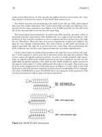
The problem can be analyzed by applying a material balance (MB) on
water across an element as shown in Figure 6.1. In this case, the water mass
balance across an elemental section between 1-1 and 2-2 gives:
Inflow at 1-1 + Recharge = Outflow at 2-2
(u × h)Խ
1
ϩ Wdx ϭ (u × h)Խ
2
Using Darcy’s equation for u and simplifying:
΄΂
–K
ᎏ
∂
∂
h
x
ᎏ
΃
× h

΅Έ
1
ϩ Wdx =
΄΂
–K
ᎏ
∂
∂
h
x
ᎏ
΃
× h
΅Έ
2
΄΂
–K
ᎏ
∂
∂
h
x
ᎏ
΃
× h
΅Έ
1
ϩ Wdx =
΄΂
–K

ᎏ
∂
∂
h
x
ᎏ
΃
× h
΅Έ
1
ϩ
ᎏ
∂
∂
x
ᎏ
΄΂
–K
ᎏ
∂
∂
h
x
ᎏ
΃
× h
΅
dx
–
ᎏ

∂
∂
x
ᎏ
΄
h
΂
–K
ᎏ
∂
∂
h
x
ᎏ
΃΅
dx ϩ Wdx = 0
∆x
x
h
h
+dh
W
∆x
q1
q2
1
1
2
2
Saturated

zone
Figure 6.1. Application of a material balance on water across an element.
Chapter 06 11/9/01 9:32 AM Page 132
© 2002 by CRC Press LLC
which has to be integrated with two BCs to solve for h. Typical BCs can be
of the form: h = h
o
at x = 0; and, h = h
1
at x = L.
Following standard mathematical calculi, the above ODE can be solved to
yield the variation of head h with x. The result is a parabolic profile
described by:
h
2
= h
2
o
ϩ
ᎏ
(h
2
L
L
– h
2
o
)
ᎏ
x ϩ

ᎏ
W
K
x
ᎏ
(L – x)
The flux at any location can now be found by determining the derivative of h
from the above result and substituting into Darcy’s equation to get:
u =
ᎏ
2
K
L
ᎏ
(h
2
o
– h
2
L
) ϩ W
΂
x –
ᎏ
L
2
ᎏ
΃
Worked Example 6.2
Two rivers,1500 m apart, fully penetrate an aquifer with a hydraulic con-

ductivity of 0.5 m/day. The water surface elevation in river 1 is 25 m, and that
in river 2 is 23 m. The average rainfall is 15 cm/yr, and the average evapora-
tion is 10 cm/yr. If a dairy is to be located between the rivers, which river is
likely to receive more loading of nitrates that might infiltrate the soil.
Solution
The equation derived in Worked Example 6.1 can be used here, measuring
x from river 1 to river 2:
u =
ᎏ
2
K
L
ᎏ
(h
2
o
– h
2
L
) ϩ W
΂
x –
ᎏ
L
2
ᎏ
΃
The flow, q, into each river can be calculated with the following data:
W = rainfall – evaporation = 15 – 10 = 5 cm/yr = 1.37 × 10
–4

m/day
K = 0.5 m/day, L = 1500 m, h
o
= 25 m, h
L
= 23 m
•
river 1: x = 0
∴u = (25 m
2
– 23 m
2
) +
΂
1.37 × 10
–4
ᎏ
d
m
ay
ᎏ
΃΂
0 –
΃
m
= –0.087
ᎏ
d
m
ay

ᎏ
The negative sign indicates that the flow is opposite to the positive
x-direction, i.e., toward river 1.
1500
ᎏ
2
0.5
ᎏ
d
m
ay
ᎏ
ᎏᎏ
2 * 1500 m
Chapter 06 11/9/01 9:32 AM Page 133
© 2002 by CRC Press LLC
•
river 2: x = 1500
∴u = (25 m
2
– 23 m
2
) +
΂
1.37 × 10
–4
ᎏ
d
m
ay

ᎏ
΃΂
1500 –
ᎏ
15
2
00
ᎏ
΃
m
= 0.12 m/day
Hence, river 2 is likely to receive a greater loading.
The problem is implemented in an Excel
®
spreadsheet to plot the head
curve between the rivers. The divide can be found analytically by setting
q = 0 and solving for x. The head will be a maximum at the divide. These con-
ditions can be observed in the plot shown in Figure 6.2 as well, from which,
at the divide, x is about 650 m.
0.5
ᎏ
d
m
ay
ᎏ
ᎏᎏ
2 * 1500 m
Figure 6.2.
Chapter 06 11/9/01 9:32 AM Page 134
© 2002 by CRC Press LLC

6.2.2 GROUNDWATER FLOW NETS
The potential theory provides a mathematical basis for understanding and
visualizing groundwater flow. A knowledge of groundwater flow can be valu-
able in preliminary analysis of fate and transport of contaminants, in screen-
ing alternate management and treatment of groundwater systems, and in their
design. Under steady, incompressible flow, the theory can be readily applied
to model various practical scenarios. Formal development of the potential
flow theory can be found in standard textbooks on hydrodynamics. The basic
equations to start from can be developed for two-dimensional flow as out-
lined below.
The continuity equation for two-dimensional flow can be developed by
considering an element to yield
ᎏ
∂
∂
u
x
ᎏ
ϩ
ᎏ
∂
∂
v
y
ᎏ
= 0 (6.6)
where u and v are the velocity components in the x- and y-directions. If a
function ψ(x,y) can be formulated such that
–
ᎏ

∂
∂
␺
y
ᎏ
= u and
ᎏ
∂
∂
␺
x
ᎏ
= v (6.7)
then the function ψ(x,y) can satisfy the above continuity equation. This func-
tion is called the stream function. This implies that if one can find the stream
function describing a flow field, then the velocity components can be found
directly by differentiating the stream function.
Likewise, another function φ(x,y) can be defined such that
–
ᎏ
∂
∂
␾
x
ᎏ
= u and –
ᎏ
∂
∂
␾

y
ᎏ
= v (6.8)
which can satisfy the two-dimensional form of the Laplace equation for flow
derived earlier, Equation (6.5). This function is called the velocity potential
function. It can also be shown that φ(x,y) = constant and ψ(x,y) = constant sat-
isfy the continuity equation and the Laplace equation for flow. In addition,
they are orthogonal to one another. In summary, the following useful rela-
tionships result:
in rectangular coordinates:
u = –
΂
ᎏ
∂
∂
␾
x
ᎏ
΃
=
΂
ᎏ
∂
∂
␺
y
ᎏ
΃
and v = –
΂

ᎏ
∂
∂
␾
y
ᎏ
΃
= –
΂
ᎏ
∂
∂
␺
x
ᎏ
΃
in cylindrical coordinates:
u
r
= –
΂
ᎏ
∂
∂
␾
r
ᎏ
΃
ϭ
ᎏ

1
r
ᎏ
΂
ᎏ
∂
∂
␺
␪
ᎏ
΃
and u
θ
= –
ᎏ
1
r
ᎏ
΂
ᎏ
∂
∂
␾
␪
ᎏ
΃
= –
΂
ᎏ
∂

∂
␺
r
ᎏ
΃
(6.9)
Chapter 06 11/9/01 9:32 AM Page 135
© 2002 by CRC Press LLC
These functions are valuable tools in groundwater studies, because they
can describe the path of a fluid particle, known as the streamline. Further,
under steady flow conditions, the two functions, φ(x,y) and ψ(x,y), are linear.
Hence, by taking advantage of the principle of superposition, functions
describing different simple flow situations can be added to derive potential
and stream functions, and hence, the streamlines for the combined flow field.
The application of the stream and potential functions and the principle of
superposition can best be illustrated by considering a practical example. The
development of the flow field around a pumping well situated in a uniform
flow field such as in a homogeneous aquifer is detailed in Worked Example
6.3, starting from the functions describing them individually.
Worked Example 6.3
Develop the stream function and the potential function to construct the
flow network for a production well located in a uniform flow field. Use the
resulting flow field to delineate the capture zone of the well.
Solution
Consider first, a uniform flow of velocity, U, at an angle, α, with the x-
direction. The velocity components in the x- and y-directions are as follows:
u = U cos ␣ and v = U sin ␣
Substituting these velocity components into the above definitions for the
potential and stream functions and integrating, the following expressions can
be derived:

␾ = ␾
0
– U(x cos ␣ + y sin ␣)
or
y = – (cos ␣)x
␺ = ␺
0
+ U(y cos ␣ – x sin ␣)
or
y =
ᎏ
u
␺
c
0
o
–
s
␺
␣
ᎏ
+ (tan ␣)x
The results indicate that the stream lines are parallel, straight lines at an angle
of α with the x-direction, which is as expected. In the special case where the
␾
0
– ␾
ᎏ
u sin ␣
Chapter 06 11/9/01 9:32 AM Page 136

© 2002 by CRC Press LLC
flow is along the x-direction, for example, with U = u, the potential and
stream functions simplify to:
␾ = ␾
0
– ux
and
␺ = ␺
0
– uy
Now, consider a well injecting or extracting a flow of ±Q located at the ori-
gin of the coordinate system. By continuity, it can be seen that the value of
Q = (2π r) u
r
, where u
r
is the radial flow velocity. Substituting this into the
definitions of the potential and stream yields in cylindrical coordinates:
␾ = ␾
0
±
ᎏ
2
Q
π
ᎏ
(ln r)
and
␺ = ␺
0

±
ᎏ
2
Q
π
ᎏ
(θ)
which can be transformed to the more familiar Cartesian coordinate system as
␾ = ␾
0
±
ᎏ
4
Q
π
ᎏ
[ln (x
2
+ y
2
)]
and
␺ = ␺
0
±
ᎏ
2
Q
π
ᎏ

tan
–1
΂
ᎏ
y
x
ᎏ
΃
The results confirm that the stream lines are a family of straight lines ema-
nating radially from the well, and the potential lines are circles with the well
at the center, as expected.
Because the stream functions and the potential functions are linear, by
applying the principle of superposition, the stream lines for the combined
flow field consisting of a production well in a uniform flow field can now be
described by the following general expression:
␺ = ␺
0
+ u(y cos ␣ – x sin ␣) ±
ᎏ
2
Q
π
ᎏ
tan
–1
΂
ᎏ
y
x
ᎏ

΃
This result is difficult to comprehend in the above abstract form; however,
a contour plot of the stream function can greatly aid in understanding the flow
pattern. Here, the Mathematica
®
equation solver package is used to model
Chapter 06 11/9/01 9:32 AM Page 137
© 2002 by CRC Press LLC
this problem. Once the basic “syntax” of Mathematica
®
becomes familiar, a
simple “code” can be written to readily generate the contours as shown in
Figure 6.3. The capture zone of the well can be defined with the aid of this plot.
Notice that the qTerm is assigned a negative sign to indicate that it is
pumping well. With the model shown, one can easily simulate various sce-
narios such as a uniform flow alone by setting the qTerm = 0 or an injection
well alone by setting u = 0 and assigning a positive sign to the qTerm or by
changing the flow directions through α.
Worked Example 6.4
Using the following potential functions for a uniform flow, a doublet, and
a source, construct the potential lines for the flow of a pond receiving
recharge with water exiting the upstream boundary of the pond. Use the fol-
lowing values: uniform velocity of the aquifer, U = 1, radius of pond, R =
200, and recharge flow, Q = 1000 π.
Uniform flow: ␾ = –ux
Doublet: ␾ =
ᎏ
x
2
R

ϩ
2
x
y
2
ᎏ
Source: ␾ = –
ᎏ
2
Q
π
ᎏ
ln [͙x
2
ϩ y
ෆ
2
ෆ
]
Figure 6.3 Groundwater flow net generated by Mathematica
®
.
Chapter 06 11/9/01 9:32 AM Page 138
© 2002 by CRC Press LLC
Solution
The potential function for the combined flow field is found by superposition:
␾ = –ux +
ᎏ
x
2

R
ϩ
2
x
y
2
ᎏ
–
ᎏ
2
Q
π
ᎏ
ln [͙x
2
ϩ y
ෆ
2
ෆ
]
The contours of constant velocity potentials can be readily constructed with
Mathematica
®
as shown in Figure 6.4. The plot shows that the stagnation
point is upstream of the pond, implying that water is exiting the upstream
boundary of the pond. This can be verified analytically by determining the
velocity u at (–R,0) and checking if it is less than zero:
u
(–R,0)
= –

΂
ᎏ
∂
∂
␾
x
ᎏ
΃
(–R,0)
ϭ
Ά
u
΄
1 –
ᎏ
x
2
R
ϩ
2
y
2
ᎏ
ϩ
ᎏ
(x
2
2
R
ϩ

2
x
y
2
2
)
2
ᎏ
΅
ϩ
ᎏ
2π(x
Q
2
ϩ
x
y
2
)
ᎏ
·
(–R,0)
The above reduces to:
u
(–R,0)
= 2u –
ᎏ
2
Q
πR

ᎏ
Figure 6.4 Contours of potential function at q = 300.
Chapter 06 11/9/01 9:32 AM Page 139
© 2002 by CRC Press LLC
giving the condition Q > 4πRu for flow to occur from the pond through its
upstream boundary. In the above example, this condition is satisfied. The con-
dition of Q < 4πRu can be readily evaluated by decreasing Q, for example,
from 1000π to 600π, and plotting the potential lines as shown in Figure 6.5.
The Mathematica
®
script can be easily adapted to superimpose the stream
function on the velocity potential function as shown in Figure 6.6, for the two
cases, to illustrate the orthogonality and to describe the flow pattern completely.
6.2.3 FLOW OF WATER AND CONTAMINANTS THROUGH
THE SATURATED ZONE
Principles of groundwater flow and process fundamentals have to be inte-
grated to model the fate and transport of contaminants in the saturated zone.
Both advective and dispersive transport of the contaminant have to be
included in the contaminant transport model, as well as the physical, biolog-
ical, and chemical reactions.
As an initial step in the analysis of contaminant transport, the ground-
water flow velocity components u, v, and w (LT
–1
), and the dispersion coef-
ficients, E
i
(L
2
T
–1

), in the direction i, can be assumed to be constant with
Figure 6.5 Contours of potential function at q = 300.
Chapter 06 11/9/01 9:32 AM Page 140
© 2002 by CRC Press LLC
space and time. A generalized three-dimensional (3-D) material balance
equation can then be formulated for an element to yield:
ᎏ
∂
∂
C
t
ᎏ
= –
΄
u
ᎏ
∂
∂
C
x
ᎏ
ϩ v
ᎏ
∂
∂
C
y
ᎏ
ϩ w
ᎏ

∂
∂
C
z
ᎏ
΅
ϩ
΄
E
x
ᎏ
∂
∂
2
x
C
2
ᎏ
ϩ E
y
ᎏ
∂
∂
2
y
C
2
ᎏ
ϩ E
z

ᎏ
∂
∂
2
z
C
2
ᎏ
΅
±
Α
r (6.10)
where the left-hand side of the equation represents the rate of change in con-
centration of the contaminant within the element, the first three terms within
the square brackets on the right-hand side represent the advective transport
across the element in the three directions, the next three terms within the next
square brackets represent dispersive transport across the element in the three
Figure 6.6 Contours of potential and stream functions at q = 500 and q = 300.
Chapter 06 11/9/01 9:32 AM Page 141
© 2002 by CRC Press LLC
directions, and the last term represents the sum of all physical, chemical, and
biological processes acting on the contaminant within the element.
An important physical process that most organic chemicals and metals
undergo in the subsurface is adsorption onto soil, resulting in their retardation
relative to the groundwater flow. For low concentrations of contaminants, this
phenomenon can be modeled assuming a linear adsorption coefficient and
can be quantified by a retardation factor, R (–), defined as follows:
R = 1 ϩ
ᎏ
K

d
n
␳
b
ᎏ
(6.11)
where K
d
is the soil-water distribution coefficient (L
3
M
–1
) = S/C, n is the
effective porosity (–), ρ
b
is the bulk density of soil (ML
–3
) = ρ
s
(1 – n), S is
the sorbed concentration (MM
–1
), and ρ
s
is the density of soil particles
(ML
–3
). Introducing the retardation factor, R, into Equation (6.10) and using
retarded velocities, uЈ, vЈ,and wЈ (LT
–1

), and retarded dispersion coefficients,
E
i
Ј
(L
2
T
–1
), results in the following:
ᎏ
∂
∂
C
t
ᎏ
= –
΄
uЈ
ᎏ
∂
∂
C
x
ᎏ
ϩ vЈ
ᎏ
∂
∂
C
y

ᎏ
ϩ wЈ
ᎏ
∂
∂
C
z
ᎏ
΅
ϩ
΄
EЈ
x
ᎏ
∂
∂
2
x
C
2
ᎏ
ϩ EЈ
y
ᎏ
∂
∂
2
y
C
2

ᎏ
ϩ EЈz
ᎏ
∂
∂
2
z
C
2
ᎏ
΅
±
ᎏ
R
1
ᎏ
Α
r (6.12)
The solution of the above PDE involves numerical procedures. However,
by invoking simplifying assumptions, some special cases can be simulated
using analytical solutions. These cases can be of benefit in preliminary eval-
uations, in screening alternative management or treatment options, in evalu-
ating and determining model parameters in laboratory studies, and in gaining
insights into the effects of the various parameters. They can also be used to
evaluate the performance of numerical models. With that note, two simplified
cases of one-dimensional flow (1-D) are given next.
Impulse input, 1-D flow with first-order consumptive reaction
A simple 1-D flow with first-order degradation reaction of the dissolved
concentration, C, such as a biological process, with a rate constant, k (T
–1

),
can be described adequately by the simplified form of Equation (6.12):
ᎏ
∂
∂
C
t
ᎏ
= –
ᎏ
R
u
ᎏ
ᎏ
∂
∂
C
x
ᎏ
ϩ
ᎏ
E
R
ᎏ
ᎏ
∂
∂
2
x
C

2
ᎏ
–
ᎏ
R
k
ᎏ
C (6.13)
For example, an accidental spill of a biodegradable chemical into the aquifer can
be simulated by treating the spill as an impulse load. For such an impulse input
Chapter 06 11/9/01 9:32 AM Page 142
© 2002 by CRC Press LLC
of mass M (M), applied at x = 0 and t = 0 to an initially pristine aquifer over an
area A (L
2
), the solution to Equation (6.13) has been reported to be as follows:
C =
΄
–
΅
΄
exp
΂
–
ᎏ
R
k
ᎏ
t
΃΅

(6.14)
Step input, 1-D flow with first-order consumptive reaction
A continuous steady release of a biodegradable chemical originating at
t = 0 into an initially pristine aquifer can also be described adequately by the
simplified Equation (6.13). For example, leakage of a biodegradable chemi-
cal into the aquifer from an underground storage tank can be simulated by
treating it as a step input load. The appropriate boundary and initial condi-
tions for such a scenario can be specified as follows:
BC: C(0, t) = C
o
for t > 0 and
ᎏ
∂
∂
C
x
ᎏ
= 0 for x = ∞
IC: C(x,0) = 0 for x ≥ 0
Under the above conditions, assuming first-order biodegradation of the dis-
solved concentration, C, the solution to Equation (6.13) has been reported to
be as follows:
C ϭ
ᎏ
C
2
o
ᎏ
Ά
exp

΄
ᎏ
(u
2
–
D
␷)
ᎏ
x
΅·Ά
erf
΄΅·
+
ᎏ
C
2
o
ᎏ
Ά
exp
΄
ᎏ
(u
2
–
D
␷)
ᎏ
x
΅·Ά

erf
΄΅·
(6.15)
where ␷ = u
Ί
1 +
ᎏ
4
u
k
๶
2
D
ᎏ
๶
Additional numerical solutions for other special cases are included in
Appendix 6.1 at the end of this chapter.
Worked Example 6.5
An underground storage tank at a gasoline station has been found to be
leaking. Considering benzene as a target component of gasoline, it is desired
to estimate the time it would take for the concentration of benzene to rise to
10 mg/L at a well located 1000 m downstream of the station. Hydraulic con-
ductivity of the aquifer is estimated as 2 m/day, effective porosity of the
aquifer is 0.2, the hydraulic gradient is 5 cm/m, and the longitudinal disper-
sivity is 8 m. Assume the initial concentration to be 800 mg/L.
(Rx – ␷ t)
ᎏ
2͙DRt
ෆ
(Rx – ␷ t)

ᎏ
2͙DRt
ෆ
΂
x –
ᎏ
R
u
ᎏ
t
΃
2
ᎏᎏ
ᎏ
4
R
Et
ᎏ
MR
ᎏᎏ
2A͙πERt
ෆ
Chapter 06 11/9/01 9:32 AM Page 143
© 2002 by CRC Press LLC
Solution
To be conservative, it may be assumed that degradation processes in the
subsurface are negligible. This situation can be modeled using the equation
given for Case 1 in Appendix 6.1:
C(L,t) ϭ
ᎏ

C
2
0
ᎏ
Ά
erfc
΄΅
– exp
΄
ᎏ
E
u
x
ᎏ
L
΅
erfc
΄΅·
The second term in the above expression is normally smaller than the first
term and, therefore, may be ignored. Using the given data,
u ϭ K =
΂
2
ᎏ
d
m
ay
ᎏ
΃
= 0.5

ᎏ
d
m
ay
ᎏ
E
x
= α
x
u = 8 m × 0.5 m/day = 4 m
2
/day
The above equation has to be solved for t, with C(L,t) = 10 mg/L; C
o
= 800
mg/L; L = 1000 m; u = 0.5 m/day; and E
x
= 4 m
2
/day:
100
ᎏ
m
L
g
ᎏ
=
Ά
erfc
΄΅·

which gives
erfc
΄΅
= 0.25 or = 0.83
The above can be readily implemented in spreadsheet or equation solver-type
software packages to solve for t. In this example, the Mathematica
®
equation
solver package is used with the built-in Solve routine as shown:
1000 m – 0.5
ᎏ
d
m
ay
ᎏ
t
ᎏᎏ
2
Ί
4
ᎏ
d
m
a
2
y
ᎏ
t
๶
1000 m – 0.5

ᎏ
d
m
ay
ᎏ
t
ᎏᎏ
2
Ί
4
ᎏ
d
m
a
2
y
ᎏ
t
๶
1000 m – 0.5
ᎏ
d
m
ay
ᎏ
t
ᎏᎏ
2
Ί
4

ᎏ
d
m
a
2
y
ᎏ
t
๶
800
ᎏ
m
L
g
ᎏ
ᎏ
2
5
ᎏ
c
m
m
ᎏ
ᎏ
100
m
cm
ᎏ
ᎏᎏ
0.2

΂
ᎏ
d
d
h
x
ᎏ
΃
ᎏ
n
L ϩ ut
ᎏ
2͙E
x
t
ෆ
L – ut
ᎏ
2͙E
x
t
ෆ
Hence, the time taken is 1724 days or 4.7 years.
Chapter 06 11/9/01 9:32 AM Page 144
© 2002 by CRC Press LLC
This example is solved in another equation solver-type package,
Mathcad
®6
, as shown in Figure 6.7. Here, a plot of C vs. t is generated from
the governing equation, from which it can be seen that the concentration at

x = 1000 m will reach 100 mg/L after about 1750 days. The plot also shows
that the peak concentration of 800 mg/L at the well will occur after about
3000 days.
6.2.4 FLOW OF WATER AND CONTAMINANTS THROUGH
THE UNSATURATED ZONE
The analysis of water flowing past the unsaturated zone, infiltration for
example, is an important consideration in irrigation, pollutant transport,
waste treatment, flow into and out of landfills, etc. Analysis of flow through
the unsaturated zone is more difficult than that of flow through the saturated
6
Mathcad
®
is a registered trademark of MathSoft Engineering & Education Inc. All rights reserved.
Figure 6.7 Mathcad
®
model of benzene concentration.
Chapter 06 11/9/01 9:32 AM Page 145
© 2002 by CRC Press LLC
zone, because the hydraulic conductivity, K, which is a function of moisture
content, θ (–), changes as the water flows through the voids. Darcy’s Law has
been shown to be valid for vertical infiltration through the unsaturated zone,
provided the K is corrected for θ as follows:
w =–K
θ
ᎏ
∂
∂
h
z
ᎏ

(6.16)
where h is the potential or head = z + ω, ω being the tension or suction (L).
For 1-D flow in the vertical direction, the water material balance for water
simplifies to:
–
΄
ᎏ
∂
∂
z
ᎏ
(ρw)
΅
=
ᎏ
∂
∂
t
ᎏ
(ρθ) (6.17)
Assuming the soil matrix is nondeformable, the water is incompressible, and
the resistance of airflow is negligible, the last two equations can be combined
to yield the following result, known as the Richard’s equation:
ᎏ
∂
∂
θ
t
ᎏ
=–

ᎏ
∂
∂
z
ᎏ
΄
K
θ
ᎏ
∂
∂
ω
z
θ
ᎏ
΅
–
ᎏ
∂
∂
K
z
θ
ᎏ
(6.18)
This nonlinear PDE is very difficult to solve, except in simple special cases
(Bedient et al., 1999). Analytical solutions reported for selected simplified
cases are given next.
Application to leachate concentration and travel time
The concentration of substances in leachates from surface spills and the

time taken for the plume to break through the vadose zone can be estimated
from the above analysis but with several simplifying assumptions as
described by Bedient et al. (1994). First, the bulk concentration, m (ML
–3
), of
the substance can be found in terms of the dissolved concentration, C (ML
–3
),
taking into account its partitioning coefficients between air-water (K
a–w
),
pure organic phase-water (K
o–w
), and soil-water (K
s–w
), and the respective
volumetric phase contents, θ
i
:
m ϭ ∏C ϭ (θ
w
ϩ K
a –w
θ
a
ϩ K
o–w
θ
o
ϩ K

s–w
␳
b
)C (6.19)
from which the total mass of the spill, M (M), can be estimated from the area
of contamination, A (L
2
), and initial depth of the spill, L
o
(L):
M ϭ AL
o
(∏C) (6.20)
Considering only the advective flow of the leachate from the contaminated
zone at a Darcy velocity of w, a material balance on the substance yields:
Chapter 06 11/9/01 9:32 AM Page 146
© 2002 by CRC Press LLC
ᎏ
d
d
M
t
ᎏ
→
ᎏ
d
d
t
ᎏ
[AL

o
∏C] → AL
o
∏
ᎏ
d
d
C
t
ᎏ
= –wAC (6.21)
which on integration with C = C
o
at t = 0 results in:
C ϭ C
o
exp
΂
–
ᎏ
L
w
o
∏
ᎏ
t
΃
(6.22)
The travel time can be estimated by assuming a power law model such as that
of Brooks and Corey to relate unsaturated hydraulic conductivity, K

θ
, to the
saturated conductivity, K. Assuming the Darcy velocity in the vertical direc-
tion to be the mean infiltration rate, W,
K
␪
ϭ K
΂
ᎏ
␪
n
–
–
␪
␪
r
r
ᎏ
΃
ε
→ ␪ = ␪
r
ϩ (n – ␪
r
)
΂
ᎏ
W
K
ᎏ

΃
ε
(6.23)
where θ is the volumetric water content, θ
r
is the irreducible minimum water
content, n is the volumetric water content at saturation, and ε is an experi-
mental parameter. Now, using Darcy’s Law and ignoring capillary pressures,
the seepage velocity, w
s
, can be approximated as follows:
w
s
= (6.24)
If R is the retardation factor defined in Equation (6.11), the retarded velocity,
wЈ (LT
–1
), can be obtained as
wЈ = (6.25)
and the travel time t
vz
through the vadose zone of length L
vz
(L) can be
found from
t
vz
=
ᎏ
L

w
v
Ј
z
ᎏ
= (6.26)
Also, if the substance undergoes a first-order degradation reaction at a rate
of k (T
–1
) as it moves through the vadose zone, then the time course of the
dissolved concentration as the plume reaches the groundwater table can be
found from
C = C
o
exp
Ά
–
΄
ᎏ
w(
L
t
o
–
∏
t
vz
)
ᎏ
ϩ kt

vz
΅·
(6.27)
΄
θ
r
ϩ (n – θ
r
)
΂
ᎏ
W
K
ᎏ
΃
1/ε
ϩ␳
b
K
d
΅
L
vz
ᎏᎏᎏᎏ
W
W
ᎏᎏᎏ
θ
r
ϩ (n – θ

r
)
΂
ᎏ
W
K
ᎏ
΃
1/ε
ϩ␳
b
k
b
W
ᎏᎏᎏ
θ
r
ϩ (n – θ
r
)
΂
ᎏ
W
K
ᎏ
΃
1/ε
Chapter 06 11/9/01 9:32 AM Page 147
© 2002 by CRC Press LLC
6.2.5 FLOW OF AIR AND CONTAMINANTS THROUGH

THE UNSATURATED ZONE
The analysis of airflow through the unsaturated zone is of particular
importance in remediation and treatment technologies, such as soil vapor
extraction, air sparging, bioventing, and biofiltration; in quantifying emis-
sions from land spills; etc. The general gas flow equation in this case can also
be developed from Darcy’s Law, and the solute transport equations can be
developed from the material balance concept.
A simplified approach to model this phenomenon, specifically for appli-
cation in soil vapor extraction, has been reported by Johnson et al. (1988).
Assuming ideal gas characteristics and horizontal flow, the following equa-
tion has been derived for radial pressure distribution around a well in the
unsaturated zone:
ᎏ
1
r
ᎏ
ᎏ
∂
∂
r
ᎏ
΂
r
ᎏ
∂(
∂
∆
r
P)
ᎏ

΃
=
΂
ᎏ
␬
␪
P
a
a
µ
tm
ᎏ
΃
ᎏ
∂
∂
∆
t
P
ᎏ
(6.28)
where r is the radial distance from the well (L); ∆P is the pressure devia-
tion from atmospheric pressure, P
atm
(ML
–1
T
–2
); θ
a

is the air-filled poros-
ity (–); µ is the viscosity of air (MLT
–1
); and κ is the intrinsic permeability
of soil (L
2
). Equation (6.28) has been solved (Johnson et al., 1990) for the
boundary condition:
r = radius of the well, R
w
P = well pressure, P
w
r = radius of influence, R
l
P = atmospheric pressure, P
atm
to get the following expression for the volumetric flow, Q, toward the well
under pressure of P
w
at the well:
Q =
΂
ᎏ
πH
µ
P
w
␬
ᎏ
΃

΄΅
(6.29)
The above result can be used to estimate the airflow Q, which in turn, can be
used in estimating the transport of volatile contaminants during soil venting,
for example. Johnson et al. (1988) proposed an equilibrium-based approach,
where two scenarios may be considered:
•
In the presence of the pure liquid phase of a contaminant in the con-
taminated zone, its concentration in the gas phase can be estimated
using Raoult’s Law to give the following:
C
a
=
ᎏ
(vp
R
)(
T
M
w
)
ᎏ
(6.30)
1 –
΂
ᎏ
P
P
a
w

tm
ᎏ
΃
2
ᎏᎏ
ln
΂
ᎏ
R
R
w
l
ᎏ
΃
Chapter 06 11/9/01 9:32 AM Page 148
© 2002 by CRC Press LLC
where vp is the vapor pressure of contaminant, M
w
is the molecular
weight of contaminant, R is the Ideal Gas Constant, and T is the
absolute temperature.
•
In the case of absence of any liquid phase of the contaminant, its con-
centration in the gas phase can be estimated assuming partitioning of
the contaminant between the soil, soil moisture, and gas phases:
C = (6.31)
where K
a–w
is the air-water partition coefficient, C
soil

is the concentra-
tion of the contaminant in the soil, θ is the moisture content, k is the
soil sorption constant, and ρ
soil
is the soil density.
The removal rate of contaminant from the soil, M, can now be estimated by
multiplying the airflow, Q, from Equation (6.29), and the gas phase concen-
tration, C, from Equation (6.30) or Equation (6.31), as M = QC.
6.3 FUNDAMENTALS OF MODELING AQUATIC SYSTEMS
Under aquatic systems, fundamental concepts relating to surface water
bodies (lakes, rivers, and estuaries) are reviewed in this section.
6.3.1 LAKE SYSTEMS
In a simple analysis of the fate of a substance discharged into a lake, the
lake can be characterized as a completely mixed system. While this assump-
tion may be justified for shallow lakes, in more sophisticated analyses, larger
lakes may be compartmentalized, and each compartment may be analyzed as
completely mixed, with interactions between compartments. It is therefore
useful to begin the modeling of lakes assuming completely mixed conditions.
In that case, because the concentration of the substance in the outlet of the
lake is the same as that inside the lake, the general form of the mass balance
equation is as follows:
ᎏ
d(V
d
t
t
C
t
)
ᎏ

= Q
in,t
C
in,t
– Q
out,t
C
t
± rV
t
(6.32)
where V
t
is the time-dependent volume of the lake (L
3
), C
t
is the time-
dependent concentration of the substance in the lake (ML
–3
), Q
in,t
is the
time-dependent volumetric flow rate into the lake (L
3
T
–1
), C
in,t
is the time-

dependent concentration of the substance in the influent (ML
–3
), Q
out,t
is the
K
a –w
C
soil
ᎏᎏ
΄
ᎏ
K
␳
a–
so
w
i
θ
l
a
ᎏ
+ θ + k
΅
Chapter 06 11/9/01 9:32 AM Page 149
© 2002 by CRC Press LLC
time-dependent volumetric flow rate out of the lake (L
3
T
–1

), r is the time-
independent reaction rate of the substance in the lake (ML
–3
T
–1
), and t is
the time (T).
As a first step in modeling a lake and simulating its response to various per-
turbations, the above general equation may be simplified by invoking the fol-
lowing assumptions: the lake volume remains constant at V, the flow rate into
and out of the lake are equal and remain constant at Q, the concentration of the
substance in the influent remains constant at C
0
, and all the reactions inside
the lake are consumptive and of first order, of rate constant, k (T
–1
). With the
above assumptions, using C instead of C
t
, Equation (6.32) reduces to:
V
ᎏ
d
d
C
t
ᎏ
= QC
in
– QC – kVC (6.33)

The above result can be rearranged to a standard mathematical form as follows:
ᎏ
d
d
C
t
ᎏ
=
ᎏ
Q
V
C
in
ᎏ
–
ᎏ
(QC ϩ
V
kVC)
ᎏ
=
ᎏ
Q
V
C
in
ᎏ
–
΂
ᎏ

Q
V
ᎏ
ϩ k
΃
C
ᎏ
d
d
C
t
ᎏ
+
΂
ᎏ
Q
V
ᎏ
ϩ k
΃
C =
ᎏ
Q
V
C
in
ᎏ
ᎏ
d
d

C
t
ᎏ
+ ␣C =
ᎏ
W
V
ᎏ
(6.34)
where
␣ =
΂
ᎏ
Q
V
ᎏ
ϩ k
΃
=
΂
ᎏ
1
τ
ᎏ
+ k
΃
(6.35)
τ =
ᎏ
Q

V
ᎏ
is the hydraulic residence time (HRT) for the lake (T) (6.36)
W = QC
in
is the load flowing into the lake (MT
–1
) (6.37)
The simplifying assumptions make it easier to analyze the response of a
lake under various loading conditions. Results from such simple analyses
help in gaining a better understanding of the dynamics of the system and its
sensitivity to the system parameters. With that understanding, further refine-
ments can be incorporated into the simple model, if necessary. In the follow-
ing sections, the application of simplified equations to several special cases
mimicking real-life situations is illustrated.
6.3.1.1 Steady State Concentration
One of the elementary scenarios that can be simulated is the steady state
condition to determine the in-lake concentration, C
ss
, of a substance caused
Chapter 06 11/9/01 9:32 AM Page 150
© 2002 by CRC Press LLC
by a continuous, constant input load of W. The steady state condition is
found by setting the first term in the left-hand side of Equation (6.22) to
zero, yielding:
C
ss
=
ᎏ
V

W
␣
ᎏ
== =
ᎏ
(1
C
ϩ
in
kτ)
ᎏ
(6.38)
6.3.1.2 General Solution
A more general situation, where the application of a new step load to a lake
with an initial concentration of C
i
causes a transient response, can be simu-
lated by Equation (6.34), giving the solution as follows (Schnoor, 1996):
C = C
o
exp
΄
–
΂
ᎏ
1
τ
ᎏ
+ k
΃

t
΅
ϩ
ᎏ
1
C
+
in
kτ
ᎏ
Ά
1 – exp
΄
–
΂
ᎏ
1
τ
ᎏ
+ k
΃
t
΅·
(6.39)
It is apparent that, by setting t to infinity, the first term in the right-hand side
of Equation (6.39) dies off to zero, and the second term approaches the steady
state value given by Equation (6.38).
The above equations can be applied to model the fate and transport of sev-
eral water quality parameters such as pathogens, BOD, dissolved oxygen,
nutrients, organic chemicals, metals, etc. Once the water column concentra-

tions of these are established from the above equations, their impacts on other
natural compartments of the lake systems such as suspended solids, biota,
fish, sediments, etc., can also be analyzed. The above results can also be
applied to simulate lakes in series, such as the Great Lakes, and compart-
mentalized lakes. Examples of such modeling are presented in the following
chapters in this book.
Worked Example 6.6
A lake of volume V of 3.15 × 10
9
ft
3
is receiving a flow, Q, of 100 cfs. A
fertilizer has been applied to the drainage basin of this lake, resulting in a
load, W, of 1080 lbs/day to the lake. The first-order decay rate K for this fer-
tilizer is 0.23 yr
–1
.
(1) Determine the steady state concentration of the chemical in the lake.
(2) If a ban is now applied on the application of the fertilizer, resulting in an
exponential decline of its inflow to the lake, this decay can be assumed
to be according to the equation W = 1080e
–µt
, where µ = 0.05 yr
–1
and t
is the time (yrs) after the ban. Develop a model to describe the concen-
tration changes in the lake.
QC
in
ᎏᎏ

V
΂
ᎏ
1
τ
ᎏ
ϩ k
΃
W
ᎏᎏ
V
΂
ᎏ
1
τ
ᎏ
ϩ k
΃
Chapter 06 11/9/01 9:32 AM Page 151
© 2002 by CRC Press LLC
Solution
(1) The steady state concentration before the ban can be found from
Equation (6.38). The detention time is first calculated as follows:
C
ss
= = = 1.63
ᎏ
m
L
g

ᎏ
(2) Assuming that the concentration in the lake has already reached 1.63
mg/L when the ban is introduced, a new MB equation has to be solved
under the declining waste load. A modified form of Equation (6.34) can
describe the system under the declining waste load:
ᎏ
d
d
C
t
ᎏ
ϩ␣C =
ᎏ
W
o
V
e
–µ t
ᎏ
The above ODE has to be solved now, with an initial condition of C =
1.63 mg/L at t = 0. Following the standard mathematical calculi of using
an integrating factor introduced in Section 3.3.2 in Chapter 3, the solu-
tion to the above can be found by applying Equation (3.18) with:
P(x) ≡ ␣
and
Q(x) ≡
ᎏ
W
V
o

ᎏ
e
–µt
Thus, the integrating factor is:
e
∫P(×)dx
= e
∫␣dt
= e
␣ t
Therefore, the solution to the ODE is as follows:
C ϭϭ
ϭ
΂
ᎏ
W
V
o
ᎏ
΃
͵
{e
(␣–µ)t
}dt ϩ b
ᎏᎏᎏ
e
␣ t
΂
ᎏ
W

V
o
ᎏ
΃
͵{e
␣ t
e
–µt
}dt ϩ b
ᎏᎏᎏ
e
␣ t
͵
Ά
e
␣ t
΂
ᎏ
W
o
V
e
–µ t
ᎏ
΃·
dt ϩ b
ᎏᎏᎏ
e
␣ t
1080

ᎏ
d
lb
a
s
y
ᎏ
΂
ᎏ
4540
lb
0
s
0mg
ᎏ
΃΂
ᎏ
365
yr
day
ᎏ
΃
ᎏᎏᎏᎏ
3.15 × 10
9
ft
3
΂
ᎏ
28.

f
3
t
3
2L
ᎏ
΃΂
ᎏ
1
1
ᎏ
+ 0.23
΃
ᎏ
y
1
r
ᎏ
W
ᎏᎏ
V
΂
ᎏ
t
1
d
ᎏ
ϩ k
΃
τ= =

×
×××






=
V
Q
315 10
100
365 24 60 60
1
9
. ft
ft
s
s
yr
yr
3
3
Chapter 06 11/9/01 9:32 AM Page 152
© 2002 by CRC Press LLC
or
C ϭ e
–␣ t
΄΂Ά

ᎏ
W
V
o
ᎏ
·
ᎏ
␣
1
– µ
ᎏ
΃
e
(␣–µ)t
ϩ b
΅
where
␣ = [(1/τ) + k] = 1.23 yr
–1
µ = 0.05 yr
–1
W
o
= 1080 lbs/day; and V = 3.5 × 10
9
ft
3
Hence, C ϭ e
–1.23t
[1.70e

1.18t
ϩ b].
The integration constant b can be found by substituting the initial condition:
C = 1.63 mg/L at t = 0,
Therefore, b = –0.07.
Hence, the concentration in the lake, C (mg/L), after the introduction of
the ban can be described by the following equation:
C = e
–1.23t
[1.70e
1.18t
– 0.07]
In Chapter 7, several variations of this problem will be modeled with dif-
ferent types of software packages.
6.3.2 RIVER SYSTEMS
In a simple analysis of the fate of a substance discharged into swiftly flow-
ing rivers and streams, river systems can be characterized as plug flow systems
with negligible dispersion. In a more realistic analysis, dispersion might have
to be included as described in the next section. Under the assumption of ideal
plug flow conditions, the water flows without any longitudinal mixing in the
direction of flow but with instantaneous mixing in all directions normal to the
flow. Thus, the concentration of substances in the water column can vary with
distance along the direction of flow as well as with time, but it is uniform at
any cross-section. Such a condition can be analyzed by setting up a differen-
tial mass balance, assuming constant flow rate and first-order reactions:
ᎏ
d(A
x
d
d

t
xC)
ᎏ
= Q
t
C – (Q
t
ϩ dQ)(C ϩ dC) ± kA
x
dxC ± S
D
A
x
dx (6.40)
where A
x
is the area of flow at a distance X from the origin (L
2
), x is the dis-
tance measured from origin along direction of flow (L), and, S
d
is the strength
of a distributed source or a sink (ML
–3
T
–1
).
Chapter 06 11/9/01 9:32 AM Page 153
© 2002 by CRC Press LLC