MODELLING OF MECHANICAL SYSTEM VOLUME 2 Episode 5 pptx
Bạn đang xem bản rút gọn của tài liệu. Xem và tải ngay bản đầy đủ của tài liệu tại đây (433.99 KB, 40 trang )
138 Structural elements
The Lagrangian is:
L =−
L
0
(E
es
+ E
eb
)dx + F
0
Z(L) = L
s
+ L
b
[3.23]
where:
L
s
=−
L
0
(E
es
)dx + F
0
Z
s
(L); L
b
=−
L
0
(E
eb
)dx + F
0
Z
b
(L)
Since the Lagrangian can be split into the sum of a shear term L
s
and a bending
term L
b
, it is anticipated that shear and bending deflections are uncoupled from
each other. Furthermore, bending is still governed by the Bernoulli–Euler model.
Hence, the variational calculation is detailed here for the shear term only:
δL
s
=−
L
0
κGS
∂Z
s
∂x
∂(δZ
s
)
∂x
dx +F
0
δZ
s
(L) = 0 [3.24]
Once more, expression [3.24] is integrated by parts and the cofactors of δZ
s
are
set to zero.
δL
s
=−
F
0
δZ
s
− κGS
∂Z
s
∂x
δZ
s
L
0
+
L
0
κGS
∂
2
Z
s
∂x
2
δZ
s
dx = 0
[3.25]
The deflection due to elastic shear is thus governed by the equation:
κGS
∂
2
Z
s
∂x
2
= 0 [3.26]
with the boundary conditions:
Z
s
(0) = 0; κGS
∂Z
s
∂x
L
= F
0
[3.27]
The system [3.26], [3.27] is consistent with equations [2.33] and [2.39], except
the shear weighting factor κ.
The total deflection is:
Z(x) = Z
s
(x) + Z
b
(x) = F
0
x
κGS
+
(3x
2
L − x
3
)
6EI
[3.28]
This result may be used to discuss the relative importance of shear and bending
deflections in relation to the slenderness ratio of the beam. Let us consider for
Straight beam models: Hamilton’s principle 139
Figure 3.3. Transverse deflection due to elastic shear and bending for two cantilever rods
(upper plot L/R =10, lower L/R =2)
instance a circular cylindrical rod of radius R and Poisson’s ratio ν = 0.3, κ =
0.95
∼
=
1. We obtain:
Z(x) =
F
0
L
πR
2
E
2(1 + ν)
x
L
+
2
3
L
2
R
2
3
x
L
2
−
x
L
3
[3.29]
The result [3.29] is evidence that the relative contribution of bending to the
total deflection increases as (L/R)
2
, validating thus the Bernoulli–Euler model for
slender beams, as illustrated in Figure 3.3.
3.2.2.3 The Rayleigh–Timoshenko dynamic model
The same problem as in the last subsection is studied now in dynamics. Focus-
ing on the case of beams of small slenderness ratios, for which shear effects are
140 Structural elements
important, the kinetic energy due to the rotation of the cross-sections with respect to
the bending axis can no longer be neglected. The kinetic energy of a cross-section
is thus written as:
E
κ
=
1
2
L
0
ρS(
˙
Z
s
+
˙
Z
b
)
2
+
1
2
ρI
∂
˙
Z
b
∂x
2
dx [3.30]
In contrast with the elastic energy, shear and bending deflections are found to
be coupled due to the cross term arising in the translational kinetic energy. The
variation of [3.30] is:
t
2
t
1
δ[E
κ
]dt = ρS
t
2
t
1
L
0
−(
¨
Z
s
+
¨
Z
b
)(δZ
s
+ δZ
b
) + ρI
∂
2
¨
Z
b
∂x
2
δZ
b
dt dx
[3.31]
Making use of the static results already derived in subsection 3.2.2.2, the
following coupled dynamic equations are found:
ρS
¨
Z −ρI
∂
2
¨
Z
b
∂x
2
+ EI
∂
4
Z
b
∂x
4
= 0
ρS
¨
Z −κGS
∂
2
Z
s
∂x
2
= 0
Z = Z
s
+ Z
b
[3.32]
Such equations can be further transformed to produce finally a single equation
expressed in terms of the sole variable Z. At first, Z
b
is eliminated from the bending
equation to produce the intermediate result:
ρS
¨
Z −ρI
∂
2
¨
Z
∂x
2
+ ρI
∂
2
¨
Z
s
∂x
2
+ EI
∂
4
Z
∂x
4
− EI
∂
4
Z
s
∂x
4
= 0 [3.33]
Then, from the second equation [3.32] we get:
∂
2
Z
s
∂x
2
=
ρ
κG
¨
Z ⇒
∂
4
Z
s
∂x
4
=
ρ
κG
∂
2
¨
Z
∂x
2
[3.34]
Relations [3.34] can be used to eliminate Z
s
from [3.33], providing thus the
final result:
ρS
∂
2
Z
∂t
2
− ρI
1 +
E
κG
∂
4
Z
∂x
2
∂t
2
+
ρ
2
I
κG
∂
4
Z
∂t
4
+ EI
∂
4
Z
∂x
4
= 0 [3.35]
Obviously, such an elimination of the variables Z
s
and Z
b
is possible only if the
beam cross-sections are uniform.
Straight beam models: Hamilton’s principle 141
3.2.3 Bending of a beam prestressed by an axial force
As is well known from common experience, the bending response of a beam can
be significantly modified when an axial force of sufficient magnitude is applied to
it. This effect is used in particular to adjust accurately the pitch of musical string
instruments. More generally, in many instances one is interested in investigating
bending resistant structures when their initial state of static equilibrium is stressed,
due to the presence of an initial loading. The variational method is particularly well
suited to modelling this kind of problem, because it brings out in a logical manner
the central importance of nonlinear strains, even if the interest is restricted to the
formulation of linear equations. Indeed, starting from an elastic medium whose
initial state of static equilibrium is characterized by the local stress tensor
σ
(0)
,
a further deformation ε referred to this initial state induces an additional stress field
denoted
σ
(1)
, and the actual stress tensor can be written as:
σ = σ
(0)
+ σ
(1)
[3.36]
The central point of the problem is to realize that when such a prestressed system
is set in motion, strain energy is varied due to the work done by the initial stress
σ
(0)
as well as that done by
σ
(1)
. Both of them are related to the Green–Lagrange strain
tensor [1.17] which comprises a linear plus a quadratic form of the displacement
gradient. On the other hand, if the aim is restricted to derive linear equations
of motion, it is suitable to approximate strain energy as a quadratic form of the
displacement derivatives, as is already the case in the absence of
σ
(0)
. Because the
elastic stress
σ
(1)
is proportional to ε, whereas the initial stress σ
(0)
is independent
of ε, it turns out that the elastic energy must be related to the linear component of
the Green–Lagrange strain tensor, whereas the prestress energy must be related to
the exact form of the Green–Lagrange strain tensor. This is further explained below
taking the example of a cantilevered beam axially stressed by a static axial force
T
0
applied initially at its free end B, see Figure 3.4.
Figure 3.4. Axially stressed cantilever
142 Structural elements
3.2.3.1 Strain energy and Lagrangian
In so far as bending is described by the Bernoulli–Euler model, the stress tensor
reduces to the axial component:
σ
xx
= σ
(0)
xx
+ σ
(1)
xx
=
T
0
S
+ Eε
xx
[3.37]
Making use of the relationship [1.47], the variation of the strain energy per unit
volume is found to be:
δ[e
s
]=σ
xx
δε
xx
=
T
0
S
+ Eε
xx
δε
xx
[3.38]
which implies:
e
s
=
T
0
S
ε
xx
+
Eε
2
xx
2
[3.39]
The longitudinal component of the Green–Lagrange tensor [1.17] is written as:
ε
xx
=
∂ξ
x
∂x
+
1
2
∂ξ
x
∂x
2
+
∂ξ
z
∂x
2
[3.40]
where ξ
z
is the local transverse displacement in the bending plane Oxz and ξ
x
is
the local axial displacement of a current point of the beam at a distance z from
the bending axis. These components are related to the global displacement field
defined in the prestressed state of equilibrium by:
ξ
z
(x, z) = Z(x); ξ
x
(x, z) =−z
∂Z
∂x
[3.41]
Substituting [3.41] into [3.40] we get:
ε
xx
=−z
∂
2
Z
∂x
2
+
1
2
∂Z
∂x
2
+
1
2
z
∂
2
Z
∂x
2
2
[3.42]
Since the aim is to derive linear equilibrium equations, it follows that strain
energy density [3.39] must be expressed as a quadratic form in terms of the Z
derivatives. Therefore, it is appropriate to use the exact form of [3.42] to formu-
late the energy involving the initial stress and to use its linear approximation to
formulate the elastic energy, which is already quadratic in ε
2
xx
. After making such
manipulations and integrating e
s
over the cross-sectional area, the following strain
Straight beam models: Hamilton’s principle 143
energy per unit beam length is obtained:
(S)
e
s
dS = T
0
+
1
2
∂Z
∂x
2
+
I
2S
∂
2
Z
∂x
2
2
+
EI
2
∂
2
Z
∂x
2
2
[3.43]
Further, if the beam is sufficiently slender, only the first term proportional to the
initial load may be retained, as the second one is less by a factor (D/L)
2
, where D
and L are the characteristic length scales in the transverse and in the axial directions
respectively. The Lagrangian of the flexed beam is thus written as:
L =
1
2
L
0
ρS
˙
Z
2
− T
0
∂Z
∂x
2
− EI
∂
2
Z
∂x
2
2
dx [3.44]
3.2.3.2 Vibration equation and boundary conditions
Starting from the Lagrangian [3.44], Hamilton’s principle is written as:
δ[A]=
t
2
t
1
dt
L
0
−
ρS
¨
ZδZ + T
0
∂Z
∂x
∂δZ
∂x
+EI
∂
2
Z
∂x
2
∂
2
δZ
∂x
2
dx = 0 [3.45]
leading to the vibration equation:
ρS
¨
Z −T
0
∂
2
Z
∂x
2
+ EI
∂
4
Z
∂x
4
= 0 [3.46]
provided with the elastic boundary conditions:
T
0
∂Z
∂x
− EI
∂
3
Z
∂x
3
δZ
L
0
= 0;
EI
∂
2
Z
∂x
2
δ
∂Z
∂x
L
0
= 0 [3.47]
In addition to the usual inertia and elastic stiffness terms, the vibration equation
includes a prestress stiffness term proportional to the initial load T
0
, which thus
may be positive or negative, depending on the sign of T
0
. On the other hand, the
first boundary condition [3.47] related to the conjugate components of transverse
shear stress and transverse displacement depends explicitly on the initial load T
0
.
In particular, if the loaded end is left free, as it is the case of the cantilevered beam,
the boundary condition at x = L is:
EI
∂
3
Z
∂x
3
− T
0
∂Z
∂x
L
= 0 [3.48]
144 Structural elements
The second boundary condition, which is related to the conjugate components of
bending moment and rotation of the cross-section, is independent of T
0
.
note. – Newtonian approach
Equations [3.46] provided with the suitable boundary conditions can also be
derived by using the Newtonian approach. However, the balance of forces and
moments must be written by referring to the deflected configuration of the beam,
contrasting with the usual case in which the non-deflected configuration of static
equilibrium is used as a reference. The effect of the preload (initial load) is shown
in Figure 3.5. The preload vector is assumed to be constant; in particular it remains
parallel to the beam axisdirection of the non-deflected configuration, independently
from the beam deflection. The forces −T
0
and T
0
act on the left- and right-hand
side cross-sections bounding the infinitesimal beam element considered. As a first
order approximation, used for projecting the forces, the small rotation of the cross-
sections is assumed to be constant in the beam element and given by −∂Z/∂x. The
projection of
T
0
onto a cross-sectional plane leads to the initial shear force:
Q
T
≃ T
s
≃ T
0
ψ
y
=−T
0
∂Z
∂x
[3.49]
The torque induced by the equilibrated axial forces ±
T
0
acting at the ends of
the beam element is:
Q
T
dx = T
0
∂Z
∂x
dx [3.50]
Figure 3.5. Bent configuration of a beam stressed axially by an initial load
Straight beam models: Hamilton’s principle 145
In agreement with the Bernoulli–Euler model, the moment balance is written as:
M
y
(x + dx) − M
y
(x) + Q
z
dx +T
0
∂Z
∂x
dx = 0 [3.51]
In so far as material behaves elastically, the resulting transverse shear force is:
Q
z
=−EI
y
∂
3
Z
∂x
3
+ T
0
∂Z
∂x
[3.52]
Substituting the expression [3.52] into the transverse equation [2.18], equa-
tion [3.46] is recovered. On the other hand, the boundary condition [3.48] is also
recovered by cancelling the shear force Q
z
at the free end of the cantilevered
beam.
3.2.3.3 Static response to a transverse force and buckling instability
The physical effect of an axial preload on the bending response of the beam can
be conveniently illustrated by solving the following static problem:
EI
d
4
Z
dx
4
− T
0
d
2
Z
dx
2
= 0
Z(0) =
dZ
dx
0
= 0;
d
2
Z
dx
2
L
= 0
EI
d
3
Z
dx
3
L
− T
0
dZ
dx
L
=−F
0
[3.53]
where the inhomogeneous boundary condition stands for a transverse force F
0
applied to the free end of the cantilevered beam.
The general solution of the homogeneous differential equation is found to be:
Z(x) = ae
k
0
x
+ be
−k
0
x
+ cx +d [3.54]
where
k
2
0
=
T
0
EI
Depending on the sign of the initial axial load T
0
, k
0
is real or purely imaginary.
Determination of the constants by using the boundary conditions of the problem
146 Structural elements
presents no difficulty and the final result may be written as:
Tensioned beam: T
0
≥ 0
Z(x) =
F
0
|T
0
|
x −
sinh(k(x −L)) +sinh(kL)
k cosh(kL)
Compressed beam: T
0
≤ 0
Z(x) =
F
0
|T
0
|
−x +
sin(k(x −L)) +sin(kL)
k cos(kL)
[3.55]
where
k =|k
0
|=
|T
0
|
EI
In Figure 3.6 the deflection of the beam is represented in a reduced form for a
few values of the tensile axial force, characterized by the dimensionless parameter
= kL = L
√
T
0
/EI , where L is the beam length and ξ = x/L is the dimension-
less abscissa along the beam. Z
m
= Z(L; = 0) is chosen as a relevant scaling
factor to reduce the beam deflection. As is conspicuous in Figure 3.6, the mag-
nitude of the deflection is significantly reduced as soon as >0.1, which means
that initial tension enhances the effective stiffness of the deflected beam, as expec-
ted. Furthermore, the shape of the deflection curves is also modified being less
curved as increases, which is a mere consequence of the increasing importance
of the tensioning term in comparison with the flexure term in the local equilibrium
equation [3.53].
Figure 3.6. Static response of a tensioned beam to a transverse force
Straight beam models: Hamilton’s principle 147
On the other hand, an initial compression decreases the effective stiffness, in
such a way that the analytical response tends to infinity for the following infinite
sequence of k values:
k
n
=
(2n + 1)π
2L
; n = 0, 1, 2 [3.56]
The physical interpretation of such a result is as follows. When the magnitude
of the compressive load is progressively increased starting from zero, the effective
stiffness of the beam is progressively reduced, leading to a larger lateral deflection
for the same transverse load F
0
, see Figure 3.7. A critical compressive load T
c
exists
for which the effective stiffnessis zero and the analyticaldeflection is infinite. Using
[3.56], T
c
is given by:
T
c
=−EI
π
2L
2
[3.57]
If the magnitude of the compressive load is further increased, according to
the mathematical model [3.53] the effective stiffness becomes negative, as can be
checked by looking at the sign of the analytical deflection [3.55], see the plots in
dashed lines of Figure 3.7. As already indicated in [AXI 04], based on a few discrete
systems such as articulated rigid bars, the axial compression of a beam can lead
to static instability, commonly called ‘buckling’ and validity of the linear model
[3.53] to describe its physical response to F
0
is strictly restricted to the subcritical
domain T
0
>T
c
.
note. – Limit case of strings and cables
Figure 3.7. Static response of a compressed beam to a transverse force
148 Structural elements
It is easily shown that in an axially prestressed beam, the relative contribution
of the flexural stiffness term to support a transverse load decreases continuously as
the slenderness of the beam increases. A dimensional analysis of equation [3.53]
gives immediately the dimensionless ratio:
elastic term
prestress term
≃
EI
T
0
L
2
∝
D
L
2
[3.58]
where again, the scale lengths D and L refer to the cross-sectional dimensions and
to the axial variation of the deflection Z(x).
Strings or cables correspond to the asymptotic and idealized case in which the
slenderness ratio of the beam is so large that bending stiffness becomes practic-
ally zero. Accordingly, their buckling resistance is also negligible; so they can
resist an external load by tensile stresses alone. In contrast with highly tensioned
strings, as those used for instance in musical instruments, most cables sag sig-
nificantly when loaded by their own weight and other in-service forces. As a
consequence, geometrical nonlinearities must often be accounted for when ana-
lysing cable systems as illustrated in Appendix A.5 where an elementary catenary
problem is solved.
3.2.3.4 Follower loads
By definition, a follower force retains the same orientation to the actual con-
figuration of the structure in the course of motion, as illustrated in Figure 3.8 in
the case of a cantilevered beam. A typical example is provided by a pressure field
applied to the wall of a flexible structure. Starting from the results established just
above, it is easy to see in which manner the preceding problem is modified if the
tensile, or compressive, force
T
0
remains tangential to the deflected beam. The
vibration equation [3.46] remains valid and the boundary condition [3.48] at a free
end reduces to the classical expression, which holds in the absence of initial axial
loading:
EI
y
∂
3
Z
∂x
3
= 0 [3.59]
Figure 3.8. Follower force applied to the free end of a cantilevered beam
Straight beam models: Hamilton’s principle 149
Hence, the static problem now takes the form:
EI
d
4
Z
dx
4
− T
0
d
2
Z
dx
2
= 0
Z(0) =
dZ
dx
0
= 0;
d
2
Z
dx
2
L
= 0
EI
d
3
Z
dx
3
L
=−F
0
[3.60]
Though at first sight the change when shifting from the system [3.53] to [3.60]
may be thought as rather benign, the nature of the problem is actually profoundly
modified. A first clue is provided by looking at the mathematical solution of [3.60].
Using the same calculation procedure as that used for solving the system [3.53] we
obtain:
1. Tensioned beam: T
0
≥ 0
Z(x) =
F
0
|T
0
|
x cosh(kL) −
sinh(k(x −L)) +sinh(kL)
k
[3.61]
2. Compressed beam: T
0
≤ 0
Z(x) =
F
0
|T
0
|
−x cos(kL) +
sin(k(x −L)) +sin(kL)
k
[3.62]
Accordingly, it is found that the beam never losses stability! However, a
closer inspection based on the concepts described in the next section shows
that even in the absence of the external force F
0
, the system [3.60] is non-
conservative, in contrast with the system [3.53]. As a consequence its beha-
viour cannot be analysed based on a static model. Study of such dynamical
problems is postponed to Volume 4. In the present example, which was invest-
igated first by Beck [BEC 52], it is found that a compressive follower force
induces a dynamical instability if its magnitude exceeds the critical value
T
c
= 2.08π
2
EI/L
2
.
3.3. Weighted integral formulations
3.3.1 Introduction
So far, for analysing the mechanical response of flexible solids, the idea
was to establish the differential equations which govern the local equilibrium
150 Structural elements
of the body and the conditions to be satisfied at the boundaries. Restrict-
ing the study to the linear domain, a set of linear partial differential equa-
tions is obtained, which can be written according to the following canonical
form:
K
X
+ C
˙
X
+ M
¨
X
=
F
(e)
(r; t) [3.63]
where K[]isthestiffness operator (matrix if the mechanical system is discrete,
differential if the system is continuous), C[]istheviscous damping operator
and M[]isthemass operator. For example, for the Bernoulli–Euler beam
model:
K[]=
∂
2
∂x
2
EI
∂
2
[]
∂x
2
; M[]=ρS[]
The operators depend on the coordinates of the Euclidean space used to
describe the geometry of the structure and they operate in a functional vector
space, namely the Hilbert space introduced in Chapter 1 subsection 1.3.2.2. On
the other hand, even if the equations [3.63] are linear, they cannot be solved
in an exact analytical way, except for a few simple configurations scarcely
encountered in practice. In most cases, approximate analytical or numerical
methods must be used to solve the problem. Amongst them, discretizing the
system [3.63] by using either the finite elements method or the projection
onto a modal basis are nowadays popular computational techniques in struc-
tural engineering. To introduce the basic theoretical aspects of these methods,
a convenient way is to start by reformulating the system [3.63] in such a
manner that the local aspect of the equations is removed. This is made pos-
sible by performing the functional scalar product of the local equation by a
weighting functional vector
W(r; t). The weighted integral formulation of con-
tinuous mechanics is introduced in subsection 3.3.2. It may be used as the
starting point of various theoretical and numerical techniques. As a first the-
oretical application, subsection 3.3.3 shows the convenience of using singular
Dirac distributions to describe local quantities as concentrated loads or sup-
port conditions. A second theoretical application, described in subsection 3.3.4
deals with the symmetry properties of the K[ ] and M[ ] operators in con-
servative systems. Such properties are a natural extension to the continuous
case of those already evidenced for discrete systems in [AXI 04]. Finally,
section 3.4 is devoted to an introductory description of the finite element
method, emphasizing the most basic and salient features of the discretization
procedure.
Straight beam models: Hamilton’s principle 151
3.3.2 Weighted equations of motion
As indicated just above, the weighted integral formulation associated with the
local system [3.63] is written as:
W ,
K
X
+ C
˙
X
+ M
¨
X
(V)
=
W ,
F
(e)
(V)
=
(V)
W ·
K
X
+ C
˙
X
+ M
¨
X
dV =
(V)
W ·
F
(e)
dV [3.64]
where use is made of a suitable weighting functional vector
W(r; t).
Again, (V) is the domain occupied by the structure. In the language of geometry,
the weighted integral formulation stands for the projection of the local equilibrium
equations [3.63] onto
W(r; t); in agreement with the relationship [1.43], the pro-
jection is carried out both onto the Euclidean geometric space (V) and onto the
functional space of the Euclidean components of the vectors. If a displacement
field is chosen for
W(r; t), the local equations [3.63] have the physical meaning
of an equilibrated balance of force densities and the weighted integral [3.64] is
interpreted in terms of energy. As a particular case, if a virtual and admissible
displacement (or velocity) field is selected for
W , [3.64] can be identified with the
formulation of the principle of virtual work, or work rate. Moreover if
W is equal
to
Xe
iωt
, the time variable can be removed and the following energy functionals
arise:
1.
X, K(r)
X
(V)
: internal (elastic and prestress) potential energy.
2.
X, C(r)
X
(V)
: viscous dissipation.
3.
X, M(r)
X
(V)
: kinetic energy.
4.
X,
F
(e)
(r; t)
(V)
: external work.
3.3.3 Concentrated loads expressed in terms of distributions
In Chapter 2 it was shown that a load concentrated at the abscissa x
0
along a
beam induces a finite discontinuity of the related global stress at x
0
. By shifting to
a weighted integral formulation of the problem, such a local effect can be described
in terms of singular Dirac distributions. The Dirac delta distributions were already
introduced in [AXI 04] Chapter 7, as a convenient analytical tool to model impulsive
loading acting at a given time t
0
on discrete systems. Here, their use is extended to
space variables, which allows one to unify the formulation of loads of any kinds,
whatever their space and time repartition may be (concentrated or not, impulsive
152 Structural elements
or not). At first, it is recalled that the Dirac distribution δ(x) is defined by the
following integral:
x
2
x
1
f(x)δ(x−x
0
)dx =
f(x
0
);ifx
0
∈[x
1
, x
2
]
0; otherwise
[3.65]
f(x) is any function complying with the sole condition that f(x
0
) exists. The
integral [3.65] may be interpreted in terms of action, by saying that it specifies the
action of the Dirac delta distribution on the ordinary function f(x).
3.3.3.1 External loads
example 1.–Beam loaded by a concentrated axial force
Let us consider again the case of a beam loaded axially by an external force
field distributed along the beam axis. It is recalled that the local equation of the
problem is:
ρS
∂
2
X
∂t
2
−
∂
∂x
ES
∂X
∂x
= F
(e)
x
(x; t)
If the external load is concentrated at some position x
0
, it may be expressed ana-
lytically as F
(e)
x
(t)δ(x −x
0
), provided that the equilibrium equation is formulated
in terms of distributions instead of ordinary functions:
ρS
∂
2
X
∂t
2
−
∂
∂x
ES
∂X
∂x
= F
(e)
x
(t)δ(x −x
0
) [3.66]
To proceed into the solution of [3.66], the necessary step is to interpret the
equation in terms of action, in a consistent way with the relation of definition [3.65].
Therefore, we shift from the local formulation [3.66] to the integral formulation:
x
2
x
1
ρS
∂
2
X
∂t
2
−
∂
∂x
ES
∂X
∂x
dx =
x
2
x
1
F
(e)
x
(t)δ(x −x
0
)dx [3.67]
Here x
1
and x
2
may be chosen arbitrarily, except that they must comply with
the condition of nonzero action of the loading, that is x
0
∈[x
1
, x
2
]. Accordingly,
the integration of [3.67] leads to:
x
2
x
1
ρS
∂
2
X
∂t
2
dx −
ES
∂X
∂x
x
2
x
1
= F
(e)
x
(t) [3.68]
Straight beam models: Hamilton’s principle 153
Because the displacement field X(x; t) is necessarily a continuous function, if
x
1
and x
2
tend towards x
0
, the action integral reduces to:
− ES
∂X
∂x
x
0
+
+ ES
∂X
∂x
x
0
−
=+F
(e)
x
(t) [3.69]
The finite jump of the axial stress at x
0
given by [3.69] is readily identified
with that given by [2.31]. Here it arises as the action of the concentrated load
on the beam. Hence the local equation [3.66] written in terms of distributions
is found to be equivalent to the following system, written in terms of ordinary
functions:
ρS
∂
2
X
∂t
2
−
∂
∂x
ES
∂X
∂x
= 0; ∀x ∈[0, L]
ES
∂X
∂x
x
0
+
− ES
∂X
∂x
x
0
−
=−F
(e)
x
(t)
[3.70]
Of course, for solving the problem, it is still necessary to use the system [3.70].
Nevertheless, the ‘symbolic’ form [3.66] is well suited to specify the discontinuity
relations arising from concentrated loads by using the local equilibrium solely. This
formalism can be generalized for other deformation modes as illustrated by the two
following examples.
example 2.–Beam loaded by a concentrated transverse force
Again, we start from the classical case of a beam bent by a transverse external
force field distributed along the beam axis. The local equation of the problem is
(see equation [2.71]):
∂
2
∂x
2
EI
y
∂
2
Z
∂x
2
+ ρS
∂
2
Z
∂t
2
= F
(e)
z
(x; t)
If the external load is concentrated at x
0
, the equation is written in terms of
distributions as:
∂
2
∂x
2
EI
y
∂
2
Z
∂x
2
+ ρS
∂
2
Z
∂t
2
= F
(e)
z
(t)δ(x −x
0
) [3.71]
154 Structural elements
A similar calculation as that made just above shows immediately that [3.71] is
equivalent to the system:
∂
2
∂x
2
EI
y
∂
2
Z
∂x
2
+ ρS
∂
2
Z
∂t
2
= 0; ∀x ∈[0, L]
∂
∂x
EI
y
∂
2
Z
∂x
2
x
0
+
−
∂
∂x
EI
y
∂
2
Z
∂x
2
x
0
−
= F
(e)
z
(t)
[3.72]
example 3.–Beam loaded by a local transverse moment
As indicated in the two last examples, it suffices to deal with the static version
of the problem. Starting thus from the local equation:
∂
2
∂x
2
EI
y
∂
2
Z
∂x
2
=
∂M
(e)
y
(x)
∂x
A moment applied at x
0
is written as the distribution M
(e)
y
(t)δ(x − x
0
). When
substituted into the right-hand side of the above equation we obtain:
∂
2
∂x
2
EI
y
∂
2
Z
∂x
2
= M
(e)
y
d(δ(x − x
0
))
dx
= M
(e)
y
δ
′
(x − x
0
) [3.73]
which is readily integrated to produce:
∂
∂x
EI
y
∂
2
Z
∂x
2
= M
(e)
y
δ(x − x
0
)
where the constant of integration can be discarded.
Performing the action integral over the interval x
0
−ε, x
0
+ε and letting ε tend
to zero the expected discontinuity follows:
EI
y
∂
2
Z
∂x
2
x
0
+
− EI
y
∂
2
Z
∂x
2
x
0
−
= M
(e)
y
[3.74]
δ
′
(x) is called the Dirac dipole. Its action on a function f(x)is obtained by integrat-
ing by parts the action of the Dirac delta on the derivative f
′
(x) which is assumed
to exist at x
0
:
x
2
x
1
f
′
(x)δ(x − x
0
)dx = f
′
(x
0
) =
[
f(x)δ(x−x
0
)
]
x
2
x
1
−
x
2
x
1
f(x)δ
′
(x − x
0
)dx
[3.75]
Straight beam models: Hamilton’s principle 155
As δ(x) is zero everywhere except at x = x
0
, it follows that the dipole action is
found to be:
x
2
x
1
f(x)δ
′
(x − x
0
)dx =
−f
′
(x
0
);ifx
0
∈[x
1
, x
2
]
0; otherwise
[3.76]
note. – Informal differentiation of δ(x)
Let us assume that the derivative of δ(x) could be defined in the same manner
as the derivative of an ordinary function. It would be thus given by the classical
limiting process:
δ
′
(x − x
0
) = lim
dx→0
δ(x + dx/2 −x
0
) − δ(x − dx/2 −x
0
)
dx
In terms of concentrated forces, this expression can be interpreted physically as
a torque of unit magnitude located at x
0
, its sign depending on the plane which is
considered, as indicated in Figure 3.9.
It can also be verified that the result arising from equations [3.74] is also con-
sistent with those sketched in Figure 2.23 of Chapter 2. On this point, reference
can also be made to the rigid rod maintained by two closely spaced knife-edged
supports, as discussed in [AXI 04] Chapter 4.
3.3.3.2 Intermediate supports
Let us consider an elastic support located at x
0
. It is characterized by a stiffness
coefficient denoted K
q
which acts on a generalized displacement q(x; t). As acorol-
lary of the results obtained in the last subsection, such a support may be described
in terms of distributions, by defining the singular stiffness operator K
q
δ(x − x
0
)
which produces the concentrated internal load K
q
q(x; t)δ(x −x
0
).
Figure 3.9. Unitary torque equivalent to a Dirac dipole
156 Structural elements
Figure 3.10. Bending of beam with multiple supports and loads
3.3.3.3 A comment on the use of distributions in mechanics
The use of the mathematical concept of distributions to describe the spatial dis-
tribution of physical quantities of any kind has the major advantage of unifying the
formulation of the equilibrium conditions, in which the necessity to make a dis-
tinction between the local equilibrium equations and the boundary or discontinuity
conditions vanishes, as illustrated by the example sketched in Figure 3.10. In terms
of distributions, the problem can be entirely formulated by writing down the sole
equation:
EI
∂
4
Z
∂x
4
+{K
1
δ(x) + K
2
δ(x − x
2
) + K
3
δ(x − L)}Z +ρS
¨
Z
=−ρgS + F
0
δ(x − x
0
)
All the local conditions are accounted for by the appropriate Dirac delta dis-
tributions. The use of the integral of action produces immediately the finite jump
conditions verified by the ordinary functions which describe the displacement and
the stress fields, and so one can proceed to the actual solution of the problem.
Finally, it can be noted that the action integral can be thought of as a weighted
integral in which the weighting function W is set to one if 0 ≤ x ≤ L, where L is
the beam length, and zero otherwise.
3.3.4 Adjoint and self-adjoint operators
As in the case of discrete systems, the dynamical behaviour of a continuous
system depends upon the physical nature of the body and contact forces involved.
In this respect, it is essential to draw a clear distinction between conservative and
nonconservative forces. It is thus expected that some counterpart has to be found
concerning the mathematical properties of the linear operators used to formulate
Straight beam models: Hamilton’s principle 157
these two kinds of forces. It is recalled (cf. for instance [AXI 04]) that the linear
stiffness and mass operators of the discrete and conservative systems are symmet-
rical matrices denoted [S], which obviously comply with the following condition
of self-adjointness:
[W ]
T
[S][X]−[X]
T
[S][W ]=0; ∀[W ], [X] [3.77]
Accordingly [S] are also termed self-adjoint matrices. Furthermore, the math-
ematical properties concerning the eigenvalues and eigenvectors of symmetrical
matrices were found to be of paramount importance for analysing the discrete
mechanical systems. Extension of such properties to the continuous case can be
made by starting from the weighted integral formulation [3.64], independently of
the dimension of the geometrical space. For mathematical convenience, it is how-
ever appropriate to discuss the problem by referring to the one-dimensional case,
which alleviates substantially the analytical notation. A linear differential operator
in a one-dimensional space is of the general form:
L[]=A
n
(x)
d
n
dx
n
+···+A
1
(x)
d
dx
+ A
0
=
n
k=0
A
k
(x)
d
k
dx
k
[3.78]
where n is the order of the differential operator and where the coefficients A
k
(x)
are assumed to be n-times differentiable functions.
In order to cope with finite discontinuities, we are interested in being able
to define the quantity L[d] even if d(x) is not a n-differentiable function. With
this aim in mind, the weighted integral L[d],
(L)
is considered. By successive
integrations by parts it is transformed into the adjoint form:
L[d],
(L)
=d,L
#
[]
(L)
[3.79]
(x)is a test function which, by definition, can be differentiated at any order
up to n, and is identically zero at the boundaries and out of the (L) domain, and so
the derivatives. L
#
[]is called the adjoint operator of L[]. It takes the form:
L
#
[]=
n
k=0
(−1)
k
d
k
(A
k
)
dx
k
[3.80]
The important point in the relationship [3.79] is that even if L[d] cannot be
defined directly because of the presence of singularities in d or its derivatives, the
adjoint form L
#
[] holds, owing to the properties of the test functions. Hence, it
is used to define the meaning of L[d], independently of the actual feasibility of the
analytical operations involved. So, the relationship [3.79] holds even if d(x) is a
distribution, singular or not.
158 Structural elements
Let us consider now the forced equation, which holds also in terms of
distributions:
L[d]=f [3.81]
By definition d(x) is a solution of [3.79] if for any test function ψ the following
equivalence holds:
L[d],
(L)
=f ,
(L)
⇐⇒ d,L
#
[]
(L)
=f ,
(L)
[3.82]
The solutions can belong to one of the two following categories:
1. d(x) can be differentiated a sufficient number of times to make the operation
L[d]actually feasible, then the solution is termed ‘classic’.
2. d(x) is not differentiable up to the required order to make the operation L[d]
feasible, then d(x) is a solution in terms of distributions, the actual meaning
of which is gained through the integral of action performed on the right-hand
side of [3.82].
On the other hand, it can happen that L[]=L
#
[]. If this is the case, the operator
is said to be formally self-adjoint and for any sufficiently regular pair of functions
u, v which vanish identically at the vicinity of the boundaries of the domain (L) –
and so the derivatives – the following equality is verified:
u, L[v]
(L)
−v, L
#
[u]
(L)
[3.83]
At this step, the property of self-adjointness is termed ‘formal’ because the
relation of equivalence [3.82] does not enforce any boundary condition. However,
if u and v, and/or their derivatives do not vanish at the boundaries, the integrations
by parts produce the following result:
u, L[v]
(L)
−v, L
#
[u]
(L)
=
[
C(u, v)
]
L
0
[3.84]
where C(u, v) is a bilinear form, called the concomitant, which depends upon the
boundary conditions.
To be self-adjoint the operator has to comply with the conditions that it is form-
ally self-adjoint, and thatit is provided with appropriate boundary conditions, which
make the concomitant disappear.
Abstract and arid as such theoretical concepts may be rightly felt, the attentive
reader can still grasp the underlying physical meaning by putting them into the
context of mechanics. Once more, if L[d]stands for a force density and u, v (or d)
for a displacement field, the integrals considered above take the physical meaning
Straight beam models: Hamilton’s principle 159
of work, which suggests that self-adjointness is a specific property of conservat-
ive operators. The easiest way for evidencing this is to apply the mathematical
formalism to a few mechanical systems.
example 1.–Viscous damping operator
Here the viscous damping operator is defined as a time differential operator:
A[]=A
∂
∂t
⇒ A
#
[]=−A
∂
∂t
It is readily found that A[ ] is not self-adjoint and more generally any odd
order operator is not self-adjoint for obvious reason of sign change included in
the integration by parts.
example 2.–Inertia operator
Defining the inertia operator as a time differential operator,
M[]=M
∂
2
∂t
2
= M
#
[]
M[ ] is formally self-adjoint as the integration by parts gives:
u, M[v] = M
+∞
−∞
u
∂
2
v
∂t
2
dt = M
[
u ˙v −v ˙u
]
+∞
−∞
+v, M[u]
Going a little bit further, the concomitant vanishes, at least at infinity for any
possible realistic motion which starts at some time and which does not last for ever.
Thus the inertia operator provided with such realistic initial and final conditions is
self-adjoint.
example 3.–Beam on elastic supports
Let us consider the bending operator of a beam, provided with elastic boundary
conditions:
K[Z]=
d
2
dx
2
EI (x)
d
2
Z
dx
2
+ elastic supports conditions
Elastic supports at the beam ends can be described either by linear relation-
ships between the conjugate displacement and stress variables, as already seen in
Chapter 2 subsection 2.2.5, or by concentrated stiffness forces as described in sub-
section 3.3.3.3. Adopting the first point of view, the elastic boundary conditions
160 Structural elements
may be written as the following linear operators:
L
1
[Z(0)]=
K
1
Z +
d
dx
EI
d
2
dx
2
Z
x=0
= 0
L
2
[Z(L)]=
K
2
Z −
d
dx
EI
d
2
dx
2
Z
x=L
= 0
L
3
[Z(0)]=
K
3
dZ
dx
+ EI
d
2
Z
dx
2
x=0
= 0
L
4
[Z(L)]=
K
4
dZ
dx
− EI
d
2
Z
dx
2
x=L
= 0
where K
1
to K
4
are the stiffness coefficients of the elastic supports.
The integration by parts of W , K[Z]
(L)
gives:
W , K[Z]
(L)
−Z, K[W ]
(L)
=
W
d
dx
EI
d
2
Z
dx
2
− Z
d
dx
EI
d
2
W
dx
2
−
dW
dx
EI
d
2
Z
dx
2
+
dZ
dx
EI
d
2
W
dx
2
L
0
Then, the operator of bending stiffness is found to be formally self-adjoint. On
the other hand, it is noted that the concomitant C(W, Z) combines the conjugate
displacement and stress variables of a flexed beam. Furthermore, the concomitant
is found to vanish if W complies with the same elastic boundary conditions L
1
to
L
4
as Z, since it takes the symmetrical form:
[WK
2
Z −ZK
2
W −W
′
K
4
Z
′
+ Z
′
K
4
W
′
]
x=L
+[WK
1
Z −ZK
1
W −W
′
K
3
Z
′
+ Z
′
K
3
W
′
]
x=0
= 0
where again the prime stands for a derivative with respect to x.
Then, the bending operator provided with elastic boundary conditions is self-
adjoint. Adopting now the concentrated force point of view, the new operator
arises:
d
2
dx
2
EI (x)
d
2
Z
dx
2
+ K
1
Z(0)δ(x) + K
2
Z(L)δ(x − L)
+ K
3
Z
′
(0)δ
′
(x) + K
4
Z
′
(L)δ
′
(x − L)
Straight beam models: Hamilton’s principle 161
Performing the action integral one obtains the same vanishing concomitant as
above.
example 4.–Cantilevered beam initially compressed by an axial force
Let us consider the operator and boundary conditions of the system [3.53]:
K[Z]=EI
d
4
Z
dx
4
− T
0
d
2
Z
dx
2
Z(0) =
dZ
dx
0
= 0;
d
2
Z
dx
2
L
= 0; EI
d
3
Z
dx
3
L
− T
0
dZ
dx
L
= 0
It is easily shown that the initial stress operator is also formally self-adjoint and
so is K[Z]. Furthermore, the concomitant [3.84] is found to be:
EI
d
3
Z
dx
3
− T
0
dZ
dx
W −
EI
d
3
W
dx
3
− T
0
dW
dx
Z
L
0
+
EI
d
2
Z
dx
2
dW
dx
− EI
d
2
W
dx
2
dZ
dx
L
0
= 0
Accordingly, bending of an axially stressed beam is described by a stiffness
operator which is self-adjoint.
example 5.–Cantilevered beam initially compressed by a follower force
Turning now to the system [3.60], the stiffness operator is the same as in the
former case, but the boundary condition relative to the transverse shear force at
the free end of the beam is changed, becoming:
EI
d
3
Z
dx
3
L
= 0
as an immediate consequence the concomitant is not zero:
EI
d
3
Z
dx
3
− T
0
dZ
dx
W −
EI
d
3
W
dx
3
− T
0
dW
dx
Z
L
0
+
EI
d
2
Z
dx
2
dW
dx
− EI
d
2
W
dx
2
dZ
dx
L
0
=
T
0
dW
dx
L
Z(L) −
T
0
dZ
dx
L
W (L) = 0
162 Structural elements
Accordingly, the bending of a beam initially stressed by a follower force is
described by a stiffness operator which is not self-adjoint, but only ‘formally’
self-adjoint and the physics of the problem is drastically changed.
3.3.5 Generic properties of conservative operators
If the study is restricted to small elastic motions in the vicinity of a static stable
(or indifferent, as a limit case) equilibrium position, the following inequalities must
be verified:
0 ≤
X, K
X
(L)
< ∞;0<
˙
X, M
˙
X
(L)
< ∞∀
X [3.85]
which means that the operators K[], M[]are respectively positive and positive
definite.
Moreover K[]and M[]are self-adjoint as can be verified in equations [3.2],
[3.3] which are quadratic symmetric forms; so the corresponding energy functionals
comply with the conditions of self-adjointness:
W , M
X
(L)
=
X, M
W
(L)
=
M
W
,
X
(L)
W , K
X
(L)
=
X, K
W
(L)
=
K
W
,
X
(L)
[3.86]
Incidentally, it is worth noticing that the relations [3.86] extend the reciprocity
theorem demonstrated by Betti which states that the virtual work of the stiffness
forces K[
W ] for an admissible displacement field
X is equal to the work done by
the forces K[
X] for the displacement field
W .
Self-adjointness is thus found to be a characteristic property of the
linear operators of conservative mechanics and the following important results
arise:
1. Any conservative problem is self-adjoint; this property characterizes not only
the operator itself but also the boundary homogeneous conditions of the prob-
lem. The interpretation in terms of energy is very clear: the mechanical energy
of a system is conserved if and only if the structure and the supports do not
exchange mechanical energy with the surroundings. This explains, in partic-
ular, why the problem of the beam stressed by an axial force differs so much
from that of a beam stressed by a follower force.
2. The mass operator is positive definite and if the static position is indifferent, or
stable, the stiffness operator is positive, or positive definite. As a consequence,
the amplitude of free oscillations in the vicinity of a stable position of static
equilibrium must be constant because the mechanical energy is also constant.