Mixed Boundary Value Problems Episode 3 pps
Bạn đang xem bản rút gọn của tài liệu. Xem và tải ngay bản đầy đủ của tài liệu tại đây (648.73 KB, 27 trang )
Historical Background 47
Using separation of variables or transform methods, the solution to Equa-
tion 2.2.1 is
u(r, z)=
∞
0
A(k)e
−k|z|
+ B(k)e
−k|z−L|
J
0
(kr)
dk
k
. (2.2.6)
This solution also satisfies the boundary conditions given by Equation 2.2.2
andEquation 2.2.3. Substituting Equation 2.2.6 into Equation 2.2.4 and
Equation 2.2.5, we obtain the dual integral equations for A(k)andB(k):
∞
0
A(k)+B(k)e
−kL
J
0
(kr)
dk
k
= V
1
, 0 ≤ r<1, (2.2.7)
∞
0
A(k)e
−kL
+ B(k)
J
0
(kr)
dk
k
= V
2
, 0 ≤ r<1, (2.2.8)
∞
0
A(k)J
0
(kr) dk =0, 1 <r<∞, (2.2.9)
and
∞
0
B(k)J
0
(kr) dk =0, 1 <r<∞. (2.2.10)
To solve Equation 2.2.9 and Equation 2.2.10, we introduce
A(k)=
2k
π
1
0
f(t)cos(kt) dt, (2.2.11)
and
B(k)=
2k
π
1
0
g(t)cos(kt) dt. (2.2.12)
To show that the A(k)givenbyEquation2.2.11 satisfies Equation 2.2.9,
we evaluate
∞
0
A(k)J
0
(kr) dk =
2
π
∞
0
1
0
f(t)k cos(kt) dt
J
0
(kr) dk (2.2.13)
=
2
π
∞
0
f(t)sin(kt)
1
0
J
0
(kr) dk
−
2
π
1
0
f
(t)
∞
0
sin(kt)J
0
(kr) dk
dt (2.2.14)
=
2
π
∞
0
f(1)sin(k)J
0
(kr) dk
−
2
π
1
0
f
(t)
∞
0
sin(kt)J
0
(kr) dk
dt (2.2.15)
=0, (2.2.16)
© 2008 by Taylor & Francis Group, LLC
48 Mixed Boundary Value Problems
because r>1andweused Equation 1.4.13. A similar demonstration holds
for B(k).
We now turn to the solution of Equation 2.2.7. Substituting Equation
2.2.11 and Equation 2.2.12 into Equation 2.2.7, we find that
1
0
f(t)
∞
0
cos(kt)J
0
(kr) dk
dt
+
1
0
g(t)
∞
0
e
−kL
cos(kt)J
0
(kr) dk
dt =
πV
1
2
. (2.2.17)
Using Equation 1.4.14, we can evaluate the first integral and obtain
h(r)+
1
0
g(τ)
∞
0
e
−kL
cos(kτ)J
0
(kr) dk
dτ =
πV
1
2
, (2.2.18)
where
h(r)=
r
0
f(t)
√
r
2
− t
2
dt. (2.2.19)
If we now multiply Equation 2.2.18 by 2rdr/
π
√
t
2
− r
2
,integratefrom0
to t,andthentaking the derivative with respect to t,wehave
f(t)+
1
0
g(τ)
2
π
d
dt
t
0
∞
0
e
−kL
cos(kτ)J
0
(kr) dk
rdr
√
t
2
− r
2
dτ
= V
1
d
dt
t
0
rdr
√
t
2
− r
2
= −V
1
d
dt
t
2
− r
2
t
0
= V
1
, (2.2.20)
since the solution to Equation 2.2.19 is
f(t)=
2
π
d
dt
t
0
rh(r)
√
t
2
− r
2
dr
. (2.2.21)
Defining
K(t, τ)=
2
π
∞
0
e
−kL
cos(kτ)
d
dt
t
0
rJ
0
(kr)
√
t
2
− r
2
dr
dk, (2.2.22)
we substitute Equation 1.4.9 into Equation 2.2.22 and K(t, τ)simplifies to
K(t, τ)=
2
π
∞
0
e
−kL
cos(kτ)cos(kt) dk (2.2.23)
=
L
π
1
L
2
+(t + τ)
2
+
1
L
2
+(t −τ)
2
. (2.2.24)
Therefore, we can write Equation 2.2.20 as
f(t)+
1
0
K(t, τ)g(τ) dτ = V
1
. (2.2.25)
© 2008 by Taylor & Francis Group, LLC
Historical Background 49
By using Equation 2.2.8, we can show in a similar manner that
g(t)+
1
0
K(t, τ)f(τ) dτ = V
2
. (2.2.26)
To evaluate u(r, z)intermsoff(t)andg(t), we substitute Equation 2.2.11
and Equation 2.2.12 into Equation 2.2.6 and find that
u(r, z)=
2
π
1
0
∞
0
f(t)e
−k|z|
+ g(t)e
−k|z−L|
cos(kt)J
0
(kr) dk
dt
(2.2.27)
=
2
π
1
0
f(t)
r
2
+(|z|−it)
2
+
g(t)
r
2
+(|z −L|+ it)
2
dt
,
(2.2.28)
where we used Equation 1.4.10.
Figure 2.2.2 illustrates u(r, z)whenL =1andV
1
= −V
2
=1. InChapter
4wewill discuss the numerical procedure used to solve Equation 2.2.25 and
Equation 2.2.26 for specific values of L, V
1
,andV
2
.WeusedSimpson’s rule
to evaluate Equation 2.2.28.
Two special cases of Equation 2.2.25 through Equation 2.2.28 are of his-
torical note. Hafen
7
solved the disc capacitor problem when the electrodes
are located at z = ± h and have a radius of a.Theelectrode at z = h has the
potential of V
1
=1while the electrode at z = −h has the potential V
2
= ±1.
He obtained
u(r, z)=
2
π
a
0
∞
0
e
−k|z−h|
± e
−k|z+h|
cos(kt)J
0
(kr) dk
f(t) dt,
(2.2.29)
where f(t)isgivenby
f(t)=1∓
2h
π
a
−a
f(τ)
(t − τ)
2
+4h
2
dτ. (2.2.30)
Hafen did not present any numerical computations.
The second special case occurs when we set V
1
= −V
2
= V
0
.Forthis
special case, Equation 2.2.25 and Equation 2.2.26 have the solution f(t)=
−g(t)=V
0
h(t), where h(t)isgivenby
h(t)=1+
1
0
K(t, τ)h(τ) dτ. (2.2.31)
7
Hafen, M., 1910: Studien ¨uber einige Probleme der Potentialtheorie. Math. Ann., 69,
517–537. See Section 3.
© 2008 by Taylor & Francis Group, LLC
Historical Background 51
occurred while solving the potential problem:
1
r
∂
∂r
r
∂u
∂r
+
1
r
2
∂
2
u
∂θ
2
=0, 0 ≤ r<∞, 0 <θ<2π, (2.3.1 )
subject to the boundary conditions
lim
r→0
|u(r, θ)| < ∞, lim
r→∞
u(r, θ) →−Vrsin(θ), 0 <θ<2π, (2.3.2)
u(1
−
,θ)=u(1
+
,θ), 0 <θ<2π, (2.3.3)
and
κu
r
(1
−
,θ)=u
r
(1
+
,θ), 0 <θ<π/2, 3π/2 <θ<2π,
u(1,θ)=0,π/2 <θ<3π/2,
(2.3.4)
where 1
−
and 1
+
denote points slightly inside and outside of the circle r =1,
respectively.
We begin by using the technique of separation of variables. This yields
the potential
u(r, θ)=−Vrsin(θ)+
∞
n=1
C
n
r
n
sin(nθ), 0 <r<1, (2.3.5 )
and
u(r, θ)=−Vrsin(θ)+
∞
n=1
C
n
r
−n
sin(nθ), 1 <r<∞. (2.3.6)
This potential satisfies not only Equation 2.3.1, but also the boundary condi-
tions given by Equations 2.3.2 and 2.3.3.
We must next satisfy the mixed boundary value condition given by Equa-
tion 2.3.4. Noting the symmetry about the x-axis, we find that we must only
consider that 0 <θ<π.Turning to the 0 <θ<π/2case,wesubstitute
Equation 2.3.5 and Equation 2.3.6 into Equation 2.3.4 and obtain
(1 + κ)
∞
n=1
nC
n
sin(nθ)=(κ − 1)V sin(θ). (2.3.7)
By integrating Equation 2.3.7 with respect to θ,wefind that
∞
n=1
C
n
cos(nθ)=
κ − 1
κ +1
V cos(θ), 0 <θ<π/2. (2.3.8)
Here, C
0
is the constant of integration.
© 2008 by Taylor & Francis Group, LLC
52 Mixed Boundary Value Problems
Let us now turn to the boundary condition for π/2 <θ<π. Substituting
Equation 2.3.5 or Equation 2.3.6 into Equation 2.3.4, we find that
∞
n=1
C
n
sin(nθ)=V sin(θ). (2.3.9)
In summary then, we solved our mixed boundary value problem, provided
that the C
n
’s satisfy Equation 2.3.8 and Equation 2.3.9.
It was the dual Fourier series given by Equation 2.3.8 and Equation 2.3.9
that motivated W. M. Shepherd
12
in the 1930s to study dual Fourier series of
the form
cos(mθ)=
∞
n=0
A
n
cos(nθ), 0 <θ<π/2, (2.3.10)
and
−sin(mθ)=
∞
n=1
A
n
sin(nθ),π/2 <θ<π, (2.3.11)
where m is a positive integer. He considered two cases: If m is an even integer,
2k,heprovedthat
A
2n
=(−1)
n+k
2k[n][k]
2k +2n
, (2.3.12)
and
A
2n+1
=(−1)
n+k
2k[n][k]
2n − 2k +1
, (2.3 .13)
where
[n]=
1 · 3 · 5 ···(2n − 1)
2 · 4 · 6 ···2n
and [0] = 1. (2.3.14)
On the other hand, if m is an odd integer, 2k +1,then
A
2n+1
=(−1)
n+k+1
(2k +1)[n][k]
2k +2n +2
, (2.3.15)
and
A
2n
=(−1)
n+k+1
(2k +1)[n][k]
2n − 2k − 1
. (2.3.16)
How can we solve Equation 2.3.7 and Equation 2.3.8 by using Shepherd’s
results? The difficulty is the (κ − 1)/(κ +1) term in Equation 2.3.8. To
12
Shepherd, W. M., 1937: On trigonometrical series with mixed conditions. Proc. Lon-
don Math. Soc., Ser. 2 , 43, 366–375.
© 2008 by Taylor & Francis Group, LLC
Historical Background 53
circumvent this difficulty, we use Equation 2.3.10 to rewrite Equation 2.3.8 as
follows:
∞
n=1
C
n
cos(nθ)=
κV
κ +1
cos(θ) −
V
κ +1
cos(θ)(2.3.17)
=
κV
κ +1
cos(θ) −
V
κ +1
∞
n=1
A
n
cos(nθ), (2.3.18)
or
∞
n=1
C
n
+
V
κ +1
A
n
cos(nθ)=
κV
κ +1
cos(θ). (2.3.19)
Similarly, we rewrite Equation 2.3.9 as follows:
∞
n=1
C
n
sin(nθ)=
κV
κ +1
sin(θ)+
V
κ +1
sin(θ)(2.3.20)
=
κV
κ +1
sin(θ) −
V
κ +1
∞
n=1
A
n
sin(nθ), (2.3.21)
or
∞
n=1
C
n
+
V
κ +1
A
n
sin(nθ)=
κV
κ +1
sin(θ). (2.3.22)
The A
n
’s are given by Equation 2.3.15 and Equation 2.3.16 with k =0. Using
either Equation 2.3.19 or 2.3.22, we equate the coefficients of each harmonic
and find that
C
1
=
2κ +1
2(κ +1)
V, C
2
= −
V
2(κ +1)
, (2.3.23)
and
C
2n−1
= −C
2n
=(−1)
n+1
1 · 3 ···(2n − 3)V
2 · 4 ···2n
. (2.3.24)
Figure 2.3.1 illustrates the solution to Equation 2.3.1 through Equation 2.3.4
when κ =6.
2.4 GRIFFITH CRACKS
During the 1920s, A. A. Griffith (1893–1963) sought to explain why a
nonductile material, such as glass, ruptures. An important aspect of his work
is the assumption that a large number of small cracks exist in the interior
of the solid body. Whether these “Griffith cracks”spreaddepends upon the
distribution of the stresses about the crack. Our interest in computing this
stress field lies in the fact that many fracture problems contain mixed bound-
ary conditions.
© 2008 by Taylor & Francis Group, LLC
Historical Background 55
and
Eγ
xy
=2(1+σ)τ
xy
, (2.4.5)
where
x
=
∂u
∂x
,
y
=
∂v
∂y
,γ
xy
=
∂u
∂y
+
∂v
∂x
, (2.4.6)
and E and σ denote the Young modulus and Poisson ratio of the material,
respectively.
The second assumption involves requiring symmetry about the y =0
plane so that our domain can be taken to be the semi-infinite plane x ≥ 0.
Taking the Fourier transform of Equation 2.4.1 through Equation 2.4.6 with
X = Y =0,wehavethat
dΣ
x
dx
+ ikT
xy
=0, (2.4.7)
dT
xy
dx
+ ikΣ
y
=0, (2.4.8)
d
2
dx
2
[Σ
y
− σ(Σ
x
+Σ
y
)] − k
2
[Σ
x
− σ(Σ
x
+Σ
y
)] = 2ik
dT
xy
dx
, (2.4.9)
ikE
1+σ
V =Σ
y
− σ(Σ
x
+Σ
y
), (2.4.10)
and
E
2(1 + σ)
dV
dx
+ ikU
= T
xy
. (2.4.11)
Remarkably these five equations can be combined together to yield
d
2
dx
2
− k
2
2
G(x, k)=0, (2.4.12)
where G(x, k)isoneofthequantities Σ
x
,Σ
y
, T
xy
, U ,orV .Thesolution of
Equation 2.4.12 which tends to zero as x →∞is
G(x, k)=[A(k)+B(k)x ]e
−|k|x
. (2.4 .13)
Finally, to evaluate the constants A(k)andB(k), we must state the
boundary condition along the crack where x =0and|y| <c.Assumingthat
the crack occurred because of the external pressure p(y), we have that
τ
xy
(0,y)=0, −∞ <y<∞, (2.4.14)
and
σ
x
(0,y)=−p(y), |y| <c,
u(0,y)=0, |y| >c,
(2.4.15)
© 2008 by Taylor & Francis Group, LLC
56 Mixed Boundary Value Problems
where p(y)isaknownevenfunction of y.Because
σ
x
(x, y)=−
1
2π
∞
−∞
P (k)(1+|k|x) e
−|k|x+iky
dk, (2.4.16)
σ
y
(x, y)=−
1
2π
∞
−∞
P (k)(1−|k|x) e
−|k|x+iky
dk, (2.4.17)
τ
xy
(x, y)=
ix
2π
∞
−∞
kP(k)e
−|k|x+iky
dk, (2.4.18)
u(x, y)=
1+σ
2πE
∞
−∞
P (k)
|k|
[2(1 − σ)+|k|x ] e
−|k|x+iky
dk, (2.4.19)
and
v(x, y)=−i
1+σ
2πE
∞
−∞
P (k)
|k|
[(1 − 2σ) −|k|x ] e
−|k|x+iky
dk, (2.4.20)
Equation 2.4.16 and Equation 2.4.19 yields the dual integral equations
2
π
∞
0
P (k)cos(ky)dk = p(y), 0 ≤ y<c, (2.4.21)
and
∞
0
P (k)cos(ky)
dk
k
=0,c<y<∞, (2.4.22)
where
P (k)=
∞
0
p(y)cos(ky) dy. (2.4.23)
How do we solve the dual integral equations, Equation 2.4.22 and Equa-
tion 2.4.23? We begin by introducing
k = ρ/c, g(η)=c
π
2η
p(cη),y= cη, (2.4.24)
and
P (ρ/c)=
√
ρF(ρ), and cos(ρη)=
πρη
2
J
−
1
2
(ρη), (2.4.25)
so that Equation 2.4.21 and Equation 2.4.22 become
∞
0
ρF (ρ)J
−
1
2
(ρη)dρ = g(η), 0 ≤ η<1, (2.4.26)
© 2008 by Taylor & Francis Group, LLC
Historical Background 57
Figure 2.4.1:Most of Ian Naismith Sneddon’s (1919–2000) life involved the University
of Glasgow. Entering at age 16, he graduated with undergraduate degrees in mathematics
and physics, returned as a lecturer in physics from 1946 to 1951, and finally accepted the
Simon Chair in Mathematics in 1956. In addition to his numerous papers, primarily on
elasticity, Sneddon published notable texts on elasticity, mixed boundary value problems,
and Fourier transforms. (Portrait from Godfrey Argent Studio, London.)
and
∞
0
F (ρ)J
−
1
2
(ρη)dρ =0, 1 ≤ η<∞. (2.4.27)
In 1938 Busbridge
13
studied the dual integral equations
∞
0
y
α
f(y)J
ν
(xy) dy = g(x), 0 ≤ x<1, (2.4.28)
and
∞
0
f(y)J
ν
(xy) dy =0, 1 ≤ x<∞, (2.4.29)
where α>−2and−ν − 1 <α−
1
2
<ν+1. He showed that
f(x)=
2
−α/2
x
−α
Γ(1 + α/2)
x
1+α/2
J
ν+α/2
(x)
1
0
y
ν+1
1 − y
2
α/2
g(y) dy
13
Busbridge, I. W., 1938: Dual integral equations. Proc. London Math. Soc., Ser. 2,
44, 115–125.
© 2008 by Taylor & Francis Group, LLC
58 Mixed Boundary Value Problems
+
1
0
η
ν+1
1 − η
2
α/2
1
0
g(ηy)(xy)
2+α/2
J
ν+1+α/2
(xy) dy
dη
.
(2.4.30)
If α>0, Sneddon
14
showed that Equation 2.4.30 simplifies to
f(x)=
(2x)
1−α/2
Γ(α/2)
1
0
η
1+α/2
J
ν+α/2
(ηx)
1
0
g(ηy)y
1+ν
1 − y
2
α/2−1
dy
dη.
(2.4.31)
In the present case, α =1,ν = −
1
2
and Equation 2.4.30 simplifies to
F (ρ)=
2ρ
π
J
0
(ρ)
1
0
y(1 −y
2
)g(y) dy
+ ρ
1
0
η(1 −η
2
)
1
0
g(ηy)y
3/2
J
1
(ρy) dy
dη
.
(2.4.32)
Asimple illustration of this solution occurs if p(y)=p
0
for all y.Then,
P (y)=p
0
cJ
1
(ck)andu(0,y)=2(1−ν
2
)
c
2
− y
2
/E.Inthiscase,thecrack
has the shape of an ellipse with semi-axes of 2(1 − ν
2
)p
0
/E and c.
2.5 THE BOUNDARY VALUE PROBLEM OF REI SSNER AND SAGOCI
Mixed boundary value problems often appear in elasticity problems. An
early example involved finding the distribution of stress within a semi-infinite
elastic medium when a load is applied to the surface z =0. Reissner and
Sagoci
15
used separation of variables and spheroidal coordinates. In 1947
Sneddon
16
resolved the static (time-independent) problems applying Hankel
transforms. This is the approach that we will highlight here.
If u(r, z)denotes the circumferential displacement, the mathematical the-
ory of elasticity yields the governing equation
∂
2
u
∂r
2
+
1
r
∂u
∂r
−
u
r
2
+
∂
2
u
∂z
2
=0, 0 ≤ r<∞, 0 <z<∞, (2.5.1)
14
See Section 12 in Sneddon, I. N., 1995: Fourier Transforms. Dover, 542pp.
15
Reissner, E., and H. F. Sagoci, 1944: Forced torsional oscillation of an elastic half-
space. J. Appl. Phys., 15, 652–654; Sagoci, H. F., 1944: Forced torsional oscillation of an
elastic half-space. II. J. Appl. Phys., 15, 655–662.
16
Sneddon, I. N., 1947: Note on a boundary value problem of Reissner and Sagoci. J.
Appl. Phys., 18, 130–132; Rahimian, M., A. K. Ghorbani-Tanha, and M. Eskandari-Ghadi,
2006: The Reissner-Sagoci problem for a transversely isotropic half-space. Int. J. Numer.
Anal. Methods Geomech., 30, 1063–1074.
© 2008 by Taylor & Francis Group, LLC
Historical Background 59
subject to the boundary conditions
lim
r→0
|u(r, z)| < ∞, lim
r→∞
u(r, z) → 0, 0 <z<∞, (2.5.2)
lim
z→∞
u(r, z) → 0, 0 ≤ r<∞, (2.5.3)
and
u(r, 0) = r, 0 ≤ r ≤ a,
u
z
(r, 0) = 0,a≤ r<∞.
(2.5.4)
Hankel transforms are used to solve Equation 2.5.1 via
U(k, z)=
∞
0
ru(r, z)J
1
(kr) dr (2.5.5)
which transforms the governing partial differential equation into the ordinary
differential equation
d
2
U(k, z)
dz
2
− k
2
U(k, z)=0, 0 <z<∞. (2.5.6)
Taking Equation 2.5.3 into account,
U(k, z)=A(k)e
−kz
. (2.5.7)
Therefore, the solution to Equation 2.5.1, Equation 2.5.2, and Equation 2.5.3
is
u(r, z)=
∞
0
kA(k)e
−kz
J
1
(kr) dk. (2.5.8)
Upon substituting Equation 2.5.8 into Equation2.5.4, we have that
∞
0
kA(k)J
1
(kr) dk = r, 0 ≤ r<a, (2 .5.9)
and
∞
0
k
2
A(k)J
1
(kr) dk =0,a<r<∞. (2.5.10)
The dual integral equations, Equation 2.5.9 and Equation 2.5.10, can be solved
using the Busbridge results, Equation2.4.28 through Equation 2.4.30. This
yields
A(k)=
4a
πk
2
sin(ak)
ak
− cos(ak)
, (2.5.11)
and
u(r, z)=
4a
π
∞
0
sin(ak)
ak
− cos(ak)
e
−kz
J
1
(kr)
dk
k
. (2.5.12)
© 2008 by Taylor & Francis Group, LLC
60 Mixed Boundary Value Problems
0
0.5
1
1.5
2
0
0.2
0.4
0.6
0.8
1
0
0.1
0.2
0.3
0.4
0.5
0.6
0.7
0.8
0.9
1
r/a
z/a
u(r,z)/a
Figure 2.5.1:Thesolutionu(r, z)/a to the mixed boundary value problem governed by
Equation 2.5.1 through Equation 2.5.4.
We can evaluate the integral in Equation 2.5.12 and it simplifies to
u(r, z)=
2a
2
rπ
λR sin(ψ + ϕ) − 2R cos(ϕ)
+
r
2
a
2
arctan
R sin(ϕ)+λ sin(ψ)
R cos(ϕ)+λ cos(ψ)
, (2.5.13)
where λ
2
sin(2ψ)tan(ψ)=2,λ
2
=1+z
2
/a
2
, z tan(ψ)=a,
R
4
=
r
2
a
2
+
z
2
a
2
− 1
2
+
4z
2
a
2
, and
2z
a
cot(2ϕ)=
r
2
a
2
+
z
2
a
2
− 1. (2.5.14)
We illustrate Equation 2.5.13 in Figure 2.5.1.
We can generalize
17
the original Reissner-Sagoci equation so that it now
reads
∂
2
u
∂r
2
+
1
r
∂u
∂r
−
u
r
2
+
∂
2
u
∂z
2
+ K
∂u
∂z
+ ω
2
u =0, 0 ≤ r<∞, 0 <z<∞,
(2.5.15)
17
See Chakraborty, S., D. S. Ray and A. Chakravarty, 1996: A dynamical problem
of Reissner-Sagoci type for a non-homogeneous elastic half-space. Indian J. Pure Appl.
Math., 27, 795–806.
© 2008 by Taylor & Francis Group, LLC
Historical Background 61
subject to the boundary conditions
lim
r→0
|u(r, z)| < ∞, lim
r→∞
u(r, z) → 0, 0 <z<∞, (2.5.16)
lim
z→∞
u(r, z) → 0, 0 ≤ r<∞, (2.5.17)
and
u(r, 0) = r, 0 ≤ r ≤ 1,
u
z
(r, 0) = 0, 1 ≤ r<∞.
(2.5.18)
If we use Hankel transforms, the solution to Equation 2.5.15 through
Equation 2.5.17 is
u(r, z)=
∞
0
A(k)e
−κ(k)z
J
1
(kr) dk, (2.5.19)
where κ(k)=K/2+
√
k
2
+ a
2
and a
2
= K
2
/4 − ω
2
.Uponsubstituting
Equation 2.5.19 into Equation 2.5.18, we have that
∞
0
A(k)J
1
(kr) dk = r, 0 ≤ r<1, (2.5.20)
and
∞
0
κ(k)A(k)J
1
(kr) dk =0, 1 <r<∞;(2.5.21)
or
∞
0
B(k)[1 + M(k)]J
1
(kr)
dk
k
=2r, 0 ≤ r<1, (2.5.22)
and
∞
0
B(k)J
1
(kr) dk =0, 1 <r<∞, (2.5.23)
where B(k)=2κ(k)A(k)andM(k)=k/κ(k) − 1.
To solve the dual integral equations, Equation 2.5.22 and Equation 2.5.23,
we set
B(k)=k
1
0
h(t)sin(kt) dt. (2.5.24)
We have done this because
∞
0
B(k)J
1
(kr) dk =
1
0
h(t)
∞
0
k sin(kt)J
1
(kr) dk
dt (2.5.25)
= −
1
0
h(t)
d
dr
∞
0
sin(kt)J
0
(kr) dk
dt =0, (2.5.26)
where we used Equation 1.4.13 and 0 ≤ t ≤ 1 <r.Consequentlyourchoice
for B(k)satisfiesEquation 2.5.23 identically.
© 2008 by Taylor & Francis Group, LLC
62 Mixed Boundary Value Problems
Turning to Equation 2.5.22, we now substitute Equation 2.5.24 and in-
terchange the order of integration:
1
0
h(t)
∞
0
sin(kt)J
1
(kr) dk
dt (2.5.27)
+
1
0
h(τ)
∞
0
M(k)sin(kτ)J
1
(kr) dk
dτ =2r.
UsingEquation 1.4.13 again, Equation 2.5.27 simplifies to
t
0
th(t)
√
r
2
− t
2
dt+
1
0
h(τ)
∞
0
M(k)sin(kτ) rJ
1
(kr) dk
dτ =2r
2
. (2.5.28)
Applying Equation 1.2.13 and Equation 1.2.14, we have
th(t)=
4
π
d
dt
t
0
η
3
t
2
− η
2
dη
(2.5.29)
−
2
π
1
0
h(τ)
∞
0
M(k)sin(kτ)
d
dt
t
0
η
2
J
1
(kη)
t
2
− η
2
dη
dk
dτ.
Now
d
dt
t
0
ξ
3
t
2
− ξ
2
dξ
=2t
2
, (2.5.30)
and
d
dt
t
0
ξ
2
J
1
(kξ)
t
2
− ξ
2
dξ
= t sin(kt)(2.5.31)
after using integral tables.
18
Substituting Equation 2.5.30 and Equation 2.5.31
into Equation 2.5.29, we finally obtain
h(t)+
2
π
1
0
h(τ)
∞
0
M(k)sin(kt)sin(kτ) dk
dτ =
8t
π
. (2.5 .32)
Equation 2.5.32 must be solved numerically. We examine this in detail in
Section 4.3. Once h(t)iscomputed, B(k)andA(k)follow from Equation
2.5.24. Finally Equation 2.5.19 gives the solution u(r, z). We illustrate this
solution in Figure 2.5.2.
18
Gradshteyn, I. S., and I. M. Ryzhik, 1965: Table of Integrals, Series, and Products .
Academic Press, Formula 6.567.1 with ν =1andµ = −
1
2
.
© 2008 by Taylor & Francis Group, LLC
64 Mixed Boundary Value Problems
Upon substituting Equation 2.5.37 into Equation 2.5.36, we obtain the triple
integral equations:
∞
0
A(k)J
1
(kr) dk = r, 0 ≤ r<a, (2.5.38)
∞
0
kA(k)J
1
(kr) dk =0,a<r<b, (2.5.39)
and
∞
0
A(k)J
1
(kr) dk =0,b<r<∞. (2.5.40)
Let us now solve this set of triple integral equations by assuming that
∞
0
kA(k)J
1
(kr) dk =
f
1
(r), 0 <r<a,
f
2
(r),b<r<∞.
(2.5.41)
Taking the inverse of the Hankel transform, we obtain from Equation 2.5.39
and Equation 2.5.41 that
A(k)=
a
0
rf
1
(r)J
1
(kr) dr +
∞
b
rf
2
(r)J
1
(kr) dr. (2.5.42)
Substituting Equation 2.5.42 into Equation 2.5.38 and Equation 2.5.40, we
find that
a
0
τf
1
(τ)L(r, τ) dτ +
∞
b
τf
2
(τ)L(r, τ) dτ = r, 0 <r<a, (2.5.43)
and
a
0
τf
1
(τ)L(r, τ) dτ +
∞
b
τf
2
(τ)L(r, τ) dτ =0,b<r<∞, (2.5.44)
where
L(r, τ)=
∞
0
J
1
(kr)J
1
(kτ) dk. (2.5.45)
At this point, we introduce several results by Cooke,
20
namely that
L(r, τ)=
2
πrτ
min(r,τ )
0
t
2
(r
2
− t
2
)(τ
2
− t
2
)
dt (2.5.46)
=
2rτ
π
∞
max(r,τ )
dt
t
2
(t
2
− r
2
)(t
2
− τ
2
)
, (2.5.47)
20
Cooke, J. C., 1963: Triple integral equations problems. Quart. J. Mech.Appl.Math.,
16, 193–201.
© 2008 by Taylor & Francis Group, LLC
Historical Background 65
b
a
min(r,τ )
0
(···) dt dτ =
r
0
b
t
(···) dτ dt +
a
0
b
a
(···) dτ dt, (2.5.48)
and
b
a
∞
max(r,τ )
(···) dt dτ =
b
r
t
a
(···) dτ dt +
∞
b
b
a
(···) dτ dt. (2.5.49)
Why have we introduced Equation 2.5.46 through Equation 2.5.49? Ap-
plying Equation 2.5.46, we can rewrite Equation 2.5.43 as
a
0
f
1
(τ)
min(r,τ )
0
t
2
(r
2
− t
2
)(τ
2
− t
2
)
dt
dτ (2.5.50)
+ r
2
∞
b
τ
2
f
2
(τ)
∞
τ
dt
t
2
(t
2
− r
2
)(t
2
− τ
2
)
dτ =
πr
2
2
for 0 <r<a.Then, applying Equation 2.5.48 and interchanging the order
of integration in the second integral, we obtain
r
0
t
2
F
1
(t)
√
r
2
− t
2
dt =
πr
2
2
− r
2
∞
b
F
2
(t)
t
2
√
t
2
− r
2
dt, 0 <r<a, (2.5.51)
where
F
1
(t)=
a
t
f
1
(τ)
√
τ
2
− t
2
dτ, 0 <t<a, (2.5.52)
and
F
2
(t)=
t
b
τ
2
f
2
(τ)
√
t
2
− τ
2
dτ, b < t < ∞. (2.5.53)
If we regard the right side of Equation 2.5.51 as a known function of r,thenit
is an integral equation of the Abel type. From Equation 1.2.13 and Equation
1.2.14, its solution is
tF
1
(t)=2t −
1
π
∞
b
2ηt
η
2
− t
2
− log
η −t
η + t
F
2
(η)
dη
η
2
, 0 <t<a,
(2.5.54)
where we used the following results:
d
dt
t
0
r
3
√
t
2
− r
2
dr
=2t
2
, (2.5.55)
and
d
dt
t
0
r
3
(t
2
− r
2
)(η
2
− r
2
)
dr
=
t
2
2ηt
η
2
− t
2
− log
η − t
η + t
. (2.5.56)
© 2008 by Taylor & Francis Group, LLC
66 Mixed Boundary Value Problems
Turning to Equation 2.5.44, we employ Equation 2.5.46 and Equation
2.5.47 and find that
∞
b
τ
2
f
2
(τ)
∞
max(r,τ )
dt
t
2
(t
2
− r
2
)(t
2
− τ
2
)
dτ (2.5.57)
+
1
r
2
a
0
f
1
(τ)
τ
0
t
2
(r
2
− t
2
)(τ
2
− t
2
)
dt
dτ =0,
if b<r<∞.Ifwenowapply Equation 2.5.49, interchange the order of inte-
gration in the second integral and use Equation 2.5.52 and Equation 2.5.53,
we find that
∞
r
F
2
(t)
t
2
√
t
2
− r
2
dt = −
1
r
2
a
0
t
2
F
1
(t)
√
r
2
− t
2
dt, b < r < ∞. (2.5.58)
Solving this integral equation of the Abel type yields
F
2
(t)
t
2
=
2
π
d
dt
∞
t
dr
r
√
r
2
− t
2
a
0
η
2
F
1
(η)
r
2
− η
2
dη
,b<t<∞.
(2.5.59)
Because
d
dt
∞
t
dr
r
(r
2
− t
2
)(r
2
− η
2
)
=
1
2ηt
2
log
t − η
t + η
−
1
t(t
2
− η
2
)
, (2.5.60)
F
2
(t)
t
=
1
π
a
0
ηF
1
(η)
1
t
log
t − η
t + η
−
2η
t
2
− η
2
dη, b < t < ∞. (2.5.61)
Setting ηF
1
(η)=2aX
1
(η), F
2
(η)/η =2aX
2
(η), c = a/b,andintroduc-
ing the variables η = bη
1
and t = at
1
,wecanrewrite Equation 2.5.54 and
Equation 2.5.59 as
X
1
(at
1
)=t
1
−
1
π
∞
1
2ct
1
η
2
1
− c
2
t
2
1
−
1
η
1
log
1 − ct
1
/η
1
1+ct
1
/η
1
X
2
(bη
1
) dη
1
,
(2.5.62)
when 0 <t
1
< 1; and
X
2
(bt
1
)=
1
π
1
0
c
t
1
log
1 − cη
1
/t
1
1+cη
1
/t
1
−
2c
2
η
1
t
2
1
− c
2
η
2
1
X
1
(aη
1
) dη
1
, (2.5.63)
when 1 <t
1
< ∞.
Once we find X
1
(at
1
)andX
2
(bt
1
)viaEquation 2.5.62 and Equation
2.5.63, we can find f
1
(r)andf
2
(r)from
f
1
(r)=−
2
π
d
dr
a
r
tF
1
(t)
√
t
2
− r
2
dt
, 0 <r<a, (2.5.64)
© 2008 by Taylor & Francis Group, LLC
Historical Background 67
0
0.5
1
1.5
2
2.5
3
0
0.2
0.4
0.6
0.8
1
0
0.1
0.2
0.3
0.4
0.5
0.6
0.7
0.8
0.9
1
r/a
z/a
u(r,z)/a
Figure 2.5.3:Thesolutionu(r, z)/a to the mixed boundary value problem governed by
Equation 2.5.33 through Equation 2.5.36 when c =
1
2
.
and
f
2
(r)=
2
πr
2
d
dr
r
b
tF
2
(t)
√
r
2
− t
2
dt
,b<r<∞. (2.5.65)
Substituting Equation 2.5.64 and Equation 2.5.65 into Equation 2.5.42 and
integrating by parts, we find that
A(k)=
4ka
3
π
1
0
1
t
X
1
(aτ)
√
τ
2
− t
2
dτ
tJ
0
(akt) dt
+
4ka
3
c
2
π
∞
1
t
1
τ
2
X
2
(bτ)
√
t
2
− τ
2
dτ
J
2
(akt/c)
t
dt. (2.5.66)
Finally, Equation 2.5.37 gives the solution u(r, z). Figure 2.5.3 illustrates this
solution when c =
1
2
.
In the previous examples of the Reissner-Sagoci problem, we solved it in
the half-space z>0. Here we solve this problem
21
within a cylinder of radius
b when the shear modulus of the materialvariesasµ
0
z
α
,where0≤ α<1.
Mathematically the problem is
∂
2
u
∂r
2
+
1
r
∂u
∂r
−
u
r
2
+
∂
2
u
∂z
2
+
α
z
∂u
∂z
=0, 0 ≤ r<b, 0 <z<∞, (2.5.67)
21
Reprinted from Int. J. Engng. Sci., 8,M.K.Kassir, The Reissner-Sagoci problem
foranon-homogeneous solid, 875–885,
c
1970, with permission from Elsevier.
© 2008 by Taylor & Francis Group, LLC
68 Mixed Boundary Value Problems
subject to the boundary conditions
lim
r→0
|u(r, z)| < ∞,u(b, z)=0, 0 <z<∞, (2.5.68)
lim
z→∞
u(r, z) → 0, 0 ≤ r<b, (2.5.69)
and
u(r, 0) = f(r), 0 ≤ r<a,
z
α
u
z
(r, z)
z=0
=0,a<r≤ b,
(2.5.70)
where b>a.
Using separation of variables, the solution to Equation 2.5.67 through
Equation 2.5.69 is
u(r, z)=z
p
∞
n=1
k
−p
n
A
n
(k
n
)K
p
(k
n
z)J
1
(k
n
r), (2.5.71)
where 2p =1− α,0<p≤
1
2
.Herek
n
denotes the nth root of J
1
(kb)=0
and n =1, 2, 3, Uponsubstituting Equation 2.5.71 into Equation 2.5.70,
we obtain the dual series:
∞
n=1
k
−2p
n
A
n
J
1
(k
n
r)=
2
1−p
Γ(p)
f(r), 0 ≤ r ≤ a, (2.5.72)
and
∞
n=1
A
n
J
1
(k
n
r)=0,a<r≤ b. (2.5.73)
Sneddon and Srivastav
22
studied dual Fourier-Bessel series of the form
∞
n=1
k
−p
n
A
n
J
ν
(k
n
ρ)=f(ρ), 0 <ρ<1, (2.5.74)
and
∞
n=1
A
n
J
ν
(k
n
ρ)=f(ρ), 1 <ρ<a. (2.5.75)
Applying here the results from their Section 4, we have that
A
n
=
2
1−p
Γ(1 − p)k
p
n
b
2
J
2
2
(k
n
b)
a
0
t
1−p
J
1−p
(k
n
t)g(t) dt. (2.5.76)
22
Sneddon, I. N., and R. P. Srivastav, 1966: Dual series relations. I. Dual relations
involving Fourier-Bessel series. Proc. R. Soc. Edinburgh, Ser. A, 66, 150–160.
© 2008 by Taylor & Francis Group, LLC
Historical Background 69
0
0.5
1
1.5
2
0
0.5
1
1.5
2
0
0.2
0.4
0.6
0.8
1
z
r
u(r,z)/ω
Figure 2.5.4:Thesolutionu(r, z)/ω to the mixed boundary value problem governed by
Equation 2.5.33 through Equation 2.5.36 when a =1,b =2andα =
1
4
.
The function g(t)isdetermined via the Fredholm integral equation of the
second kind
g(t)=h(t)+
2
π
sin(πp)t
p
a
0
τ
1−p
g(τ)L(t, τ) dτ, (2.5.77)
where
h(t)=
2
1+p
sin(πp)
πΓ(1 −p)
t
2p−1
1
0
d
dr
rf(r)
dr
(t
2
− r
2
)
p
, (2.5.78)
and
L(t, τ )=
∞
0
K
1
(by)
I
1
(by)
I
1−p
(ty)I
1−p
(τy) ydy. (2.5.79)
To illustrate our results, we choose f(r)=ωr.Then
h(t)=
2
1+p
ω sin(πp)
πΓ(2 −p)
t. (2.5.80)
Figure 2.5.4 illustrates the case when a =1,b =2andα =
1
4
.
Problems
1. Solve Helmholtz’s equation
∂
2
u
∂r
2
+
1
r
∂u
∂r
+
∂
2
u
∂z
2
−
α
2
+
1
r
2
u =0, 0 ≤ r<∞, 0 <z<∞,
© 2008 by Taylor & Francis Group, LLC
70 Mixed Boundary Value Problems
subject to the boundary conditions
lim
r→0
|u(r, z)| < ∞, lim
r→∞
u(r, z) → 0, 0 <z<∞,
lim
z→∞
u(r, z) → 0, 0 ≤ r<∞,
and
u(r, 0) = q(r), 0 ≤ r<1,
u
z
(r, 0) = 0, 1 <r<∞.
Step 1 : Show that the solution to the differential equation plus the first three
boundary conditions is
u(r, z)=
∞
0
A(k)e
−z
√
k
2
+α
2
J
1
(kr) dk.
Step 2 :Using the last boundary condition, show that we obtain the dual
integral equations
∞
0
A(k)J
1
(kr) dk = q(r), 0 ≤ r<1,
and
∞
0
k
2
+ α
2
A(k)J
1
(kr) dk =0, 1 <r<∞.
Step 3 :If
√
k
2
+ α
2
A(k)=kB(k), then the dual integral equations become
∞
0
k
√
k
2
+ α
2
B(k)J
1
(kr) dk = q(r), 0 ≤ r<1,
and
∞
0
kB(k)J
1
(kr) dk =0, 1 <r<∞.
Step 4 :Considerthe first integral equation in Step 3. By multiplying both
sides of this equation by dr/
√
t
2
− r
2
,integratingfrom0tot and using
t
0
J
1
(kr)
√
t
2
− r
2
dr =
1 − cos(kt)
kt
,
show that
∞
0
k
√
k
2
+ α
2
B(k)
1 − cos(kt)
kt
dk =
t
0
q(r)
√
t
2
− r
2
dr, 0 ≤ t<1,
© 2008 by Taylor & Francis Group, LLC
Historical Background 71
or
∞
0
k
√
k
2
+ α
2
B(k)sin(kt) dk =
d
dt
t
0
tq(r)
√
t
2
− r
2
dr
, 0 ≤ t<1.
Step 5 :Considernextthesecond integral equation in Step 3. By multiplying
both sides by dr/
√
r
2
− t
2
,integratingfromt to ∞ and using
∞
t
J
1
(kr)
√
r
2
− t
2
dr =
sin(kt)
kt
,
show that
∞
0
B(k)sin(kt) dk =0, 1 ≤ t<∞.
Step 6 :Ifweintroduce
g(t)=
∞
0
B(k)sin(kt) dk,
show that the integral equations in Step 4 and Step 5 become
g(t) −
∞
0
1 −
k
√
k
2
+ α
2
B(k)sin(kt) dk =
d
dt
t
0
tq(r)
√
t
2
− r
2
dr
,
for 0 ≤ t<1, and
g(t)=0, 1 <t<∞.
Step 7 :Because
B(k)=
2
π
1
0
g(t)sin(kt) dt,
show that the function g(t)isgovernedby
g(t) −
2
π
1
0
g(τ)
∞
0
1 −
k
√
k
2
+ α
2
sin(kt)sin(kτ) dk
dτ
=
d
dt
t
0
tq(r)
√
t
2
− r
2
dr
for 0 ≤ t<1. Once g(t)iscomputed numerically, then B(k)andA(k)follow.
Finally, the values of A(k)areusedintheintegral solutiongivenin Step 1.
© 2008 by Taylor & Francis Group, LLC
72 Mixed Boundary Value Problems
0
0.5
1
1.5
2
0
0.2
0.4
0.6
0.8
1
0
0.2
0.4
0.6
0.8
1
z
r
u(r,z)
Problem 1
Step 8:Takingthe limit as α → 0, show that you recover the solution given
by Equation 2.5.11 and Equation 2.5.12 with a =1andq(r)=r.Inthefigure
labeled Problem 1, we illustrate the solution when α =1andq(r)=r.
2.6 STEADY ROTATIONOFACIRCULARDISC
Aproblem that is similar to the Reissner-Sagoci problem involves finding
the steady-state velocity field within a laminar, infinitely deep fluid that is
driven by a slowly rotating disc of radius a in contact with the free surface.
The discrotates at the angular velocity ω.TheNavier-Stokesequationsfor
the angular component u(r, z)ofthefluid’s velocity reduce to
∂
2
u
∂r
2
+
1
r
∂u
∂r
−
u
r
2
+
∂
2
u
∂z
2
=0, 0 ≤ r<∞, 0 <z<∞. (2.6.1)
At infinity the velocity must tend to zero which yields the boundary conditions
lim
r→0
|u(r, z)| < ∞, lim
r→∞
u(r, z) → 0, 0 <z<∞, (2.6.2)
and
lim
z→∞
u(r, z) → 0, 0 ≤ r<∞. (2.6.3)
At the interface, the mixed boundary condition is
u(r, 0) = ωr, 0 ≤ r<a,
µu
z
(r, 0) + ηu
zz
(r, 0) = 0,a<r<∞.
(2.6.4)
Goodrich
23
was the first to attack this problem. Using Hankel transforms,
the solution to Equation 2.6.1 through Equation 2.6.3 is
u(r, z)=
∞
0
A(k)J
1
(kr)e
−kz
dk. (2.6.5)
23
Takenwithpermission from Goodrich, F. C., 1969: The theory of absolute surface
shear viscosity. I. Proc. Roy. Soc. London, Ser. A, 310, 359–372.
© 2008 by Taylor & Francis Group, LLC
Historical Background 73
Substituting Equation 2.6.5 into Equation 2.6.4, we have that
∞
0
A(k)J
1
(kr) dk = ωr, 0 ≤ r<a, (2.6.6)
and
∞
0
(ηk
2
− µk)A(k)J
1
(kr) dk =0,a<r<∞. (2.6.7)
Before Goodrich tackled the general problem, he considered the following
special cases.
µ =0
In this special case, Equation 2.6.6 and Equation 2.6.7 simplify to
∞
0
A(k)J
1
(kr) dk = ωr, 0 ≤ r<a, (2.6.8)
and
∞
0
k
2
A(k)J
1
(kr) dk =0,a<r<∞. (2.6.9)
Now, multiplying Equation 2.6.8 by r and differentiating with respect to r,
∞
0
A(k)
d
dr
[rJ
1
(kr)] dk =2ωr, 0 ≤ r<a. (2.6.10)
In the case of Equation 2.6.9, integrating both sides with respect to r,we
obtain
∞
0
k
2
A(k)
∞
r
J
1
(kξ) dξ
dk =0,a<r<∞. (2.6.11)
From the theory of Bessel functions,
24
d
dr
[rJ
1
(kr)] = krJ
0
(kr), (2.6.12)
and
∞
r
J
1
(kξ) dξ =
J
0
(kr)
k
. (2.6.13)
Substituting Equation 2.6.12 and Equation 2.6.13 into Equation 2.6.10 and
Equation 2.6.11, respectively, they become
∞
0
kA(k)J
0
(kr) dk =2ω, 0 ≤ r<a, (2.6.14)
24
Gradshteyn and Ryzhik, op. cit., Formulas 8.472.3 and 8.473.4 with z = kr.
© 2008 by Taylor & Francis Group, LLC
74 Mixed Boundary Value Problems
0
0.5
1
1.5
2
0
0.5
1
1.5
2
0
0.1
0.2
0.3
0.4
0.5
0.6
0.7
0.8
0.9
1
z/a
r/a
u(r,z)/(ω a)
Figure 2.6.1:The solution to Laplace’s equation, Equation 2.6.1, with the boundary
conditions given by Equation 2.6.2 through Equation 2.6.4 when µ =0.
and
∞
0
kA(k)J
0
(kr) dk =0,a<r<∞. (2.6.15)
Taking the inverse Hankel transform given by Equation 2.6.14 and Equation
2.6.15, we have that
A(k)=2ω
a
0
rJ
0
(kr) dr =2ωa
J
1
(ak)
k
. (2.6.16)
Therefore,
u(r, z)=2ωa
∞
0
J
1
(ξ)J
1
(ξr/a)e
−ξz/a
dξ
ξ
. (2.6.17)
Figure 2.6.1 illustrates this solution.
η =0
In this case Equation 2.6.6 and Equation 2.6.7 become
∞
0
A(k)J
1
(kr) dk = ωr, 0 ≤ r<a, (2.6.18)
and
∞
0
kA(k)J
1
(kr) dk =0,a<r<∞. (2.6.19)
If we now introduce a function g(r)suchthat
∞
0
kA(k)J
1
(kr) dk = g(r), 0 ≤ r<a, (2.6.20)
© 2008 by Taylor & Francis Group, LLC