Mixed Boundary Value Problems Episode 8 ppsx

198 Mixed Boundary Value Problems
−4
−2
0
2
4
0
1
2
−1
−0.5
0
0.5
1
x
y
u(x,y)
Problem 2
and

∞
0
A(k)sin(kx) dk =0, 1 < |x| < ∞.
Step 3:Fredricks
27
showed that dual integral equations of the form

∞
0
A(k)
k

sin(kx) dk = f(x), 0 ≤ x<a,
and

∞
0
A(k)sin(kx) dk =0,a<x<∞,
have the solution
A(k)=2
∞

n=1
∞

m=0
(2m +1)B
n
J
2m+1
(nπ)J
2m+1
(ka),
where B
n
is given by the Fourier sine series
f(x)=
∞

n=1
B
n

sin(nπx/a), 0 ≤ x<a.
Clearly f(0) = 0. Use this result to show that
A(k)=
4
π
∞

n=1
∞

m=0
(−1)
n+1
n
(2m +1)B
n
J
2m+1
(nπ)J
2m+1
(k).
The figure labeled Problem 2 illustrates this solution u(x, y).
27
Fredricks, R. W., 1958: Solution of a pair of integral equations from elastostatics.
Proc. Natl. Acad. Sci., 44, 309–312. See also Sneddon, I. N., 1962: Dual integral
equations with trigonometrical kernels. Proc. Glasgow Math. Assoc., 5, 147–152.
© 2008 by Taylor & Francis Group, LLC
Transform Methods 199
3. Following Example 4.1.3, solve Laplace’s equation
∂

2
u
∂x
2
+
∂
2
u
∂y
2
=0, 0 <x<∞, 0 <y<h,
with the boundary conditions
u
x
(0,y)=0, lim
x→∞
u(x, y) → 0, 0 <y<h,

u
y
(x, 0) = −g(x), 0 <x<a,
u(x, 0) = 0,a<x<∞,
(1)
and
u(x, h)=0, 0 <x<∞.
Step 1 :Usingseparation of variables or transform methods, show that the
general solution totheproblem is
u(x, y)=
2
π


∞
0
A(k)sinh[k(h −y)] cos(kx) dk.
Step 2:Using boundary condition (1), show that A(k)satisfiesthe dual inte-
gral equations
2
π

∞
0
kA(k)[1+M(kh)] sinh(kh)cos(kx) dk = g(x), 0 <x<a,
and
2
π

∞
0
A(k)sinh(kh)cos(kx) dk =0,a<x<∞,
where M(kh)=e
−kh
/ sinh(kh).
Step 3:Setting
sinh(kh)A(k)=

a
0
τh(τ)J
0
(kτ)dτ,

show that the second integral equation in Step 2 is identically satisfied.
Step 4 : Show that the first integral equation in Step 2 leads to the integral
equation
h(t)+

a
0
τh(τ)


∞
0
kM(kh)J
0
(kτ)J
0
(kt) dk

dτ =

t
0
g(x)
√
t
2
− x
2
dx
with 0 <t<a.

Step 5 :Simplify your results in the case g(x)=1andshowthat they are
identical with the results given in Example 4.1.3 by Equation 4.1.83 through
Equation 4.1.86.
© 2008 by Taylor & Francis Group, LLC
200 Mixed Boundary Value Problems
4. Following Example 4.1.2, solve Laplace’s equation
28
∂
2
u
∂x
2
+
∂
2
u
∂y
2
=0, −∞ <x<∞, 0 <y<h,
with the boundary conditions
lim
|x|→∞
u(x, y) → 0, 0 <y<h,

u
y
(x, 0) = −p(x)/h, |x| <a,
u(x, 0) = 0, |x| >a,
(1)
and

u(x, h)=0, −∞ <x<∞.
Step 1 :Usingseparation of variables or transform methods, show that the
general solution totheproblem is
u(x, y)=
2
π

∞
0
A(k)
e
−ky
− e
ky−2kh
1 − e
−2kh
cos(kx) dk.
Step 2:Using boundary condition (1), show that A(k)satisfiesthe dual inte-
gral equations
2
π

∞
0
k coth(kh)A(k)cos(kx) dk =
p(x)
h
, |x| <a,
and
2

π

∞
0
A(k)cos(kx) dk =0, |x| >a.
Step 3:Setting
kA(k)=
π
2

a
0
g(τ)sin(kτ) dτ,
show that the second integral equation in Step 2 is identically satisfied.
Step 4: Show that the first integral equation in Step 2 can be rewritten
d
dx


a
0
g(τ)


∞
0
coth(kh)sin(kτ)sin(kx)
dk
k


dτ

=
p(x)
h
, 0 <x<a.
28
Suggested from Singh, B. M., T. B. Moodie, and J. B. Haddow, 1981: Closed-form
solutions for finite length crack moving in a strip under anti-plane shear stress. Acta Mech.,
38, 99–109.
© 2008 by Taylor & Francis Group, LLC
Transform Methods 201
−3
−2
−1
0
1
2
3
0
0.5
1
1.5
2
−0.05
0
0.05
0.1
0.15
0.2

0.25
0.3
0.35
0.4
0.45
x
y
u(x,y)/p
0
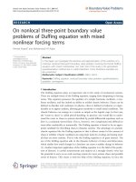
Problem 4
Step 5:Usingtherelationship that

∞
0
coth(kh)sin(kτ)sin(kx)
dk
k
=
1
2
ln




tanh(cx)+tanh(cτ)
tanh(cx) − tanh(cτ)





,
where c = π/(2h), show that Step 4 can be written

a
0
g(τ)ln




tanh(cx)+tanh(cτ)
tanh(cx) − tanh(cτ)




dτ =
2
h

x
0
p(ξ) dξ = F (x), 0 <x<a.
Step 6 :Byusingtheresults from Example 1.2.3, show that the solution to
the integral equation in Step 5 is
g(τ)=−
2c tanh(cτ)sech
2
(cτ)

π
2

tanh
2
(ca) −tanh
2
(cτ)

a
0
F

(x)

tanh
2
(ca) − tanh
2
(cx)
tanh
2
(cx) −tanh
2
(cτ)
dx
+
4cF (0) tanh(ca)
π
2

sinh(2cτ)

tanh
2
(ca) − tanh
2
(cτ)
, 0 <τ<a.
Step 7:Because F

(x)=2p(x)/h with F (0) = 0, show that Step 6 simplifies
to
g(τ)=−
4c tanh(cτ)sech
2
(cτ)
π
2
h

tanh
2
(ca) − tanh
2
(cτ)

a
0
p(x)


tanh
2
(ca) − tanh
2
(cx)
tanh
2
(cx) − tanh
2
(cτ)
dx,
if 0 <τ <a.
Step 8:Forthespecial case p(x)=p
0
,aconstant,showthat
g(τ)=
2p
0
sinh(cτ)
πh

sinh
2
(ca) − sinh
2
(cτ)
, 0 <τ <a.
The figure entitled Problem 4 illustrates this special solution when a =1and
h =2.
© 2008 by Taylor & Francis Group, LLC

202 Mixed Boundary Value Problems
4.2 TRIPLE FOURIER INTEGRALS
In the previous section we considered the case where the mixed boundary
conditions led to two integral equations that are in the form of a Fourier inte-
gral. In the present section we take the next step and examine the situation
where the mixed boundary condition contains different boundary conditions
along three segments.
• Example 4.2.1
For our first example, let us solve Laplace’s equation
∂
2
u
∂x
2
+
∂
2
u
∂y
2
=0, −∞ <x<∞, 0 <y<∞, (4.2.1)
subject to the boundary conditions
lim
|x|→∞
u(x, y) → 0, 0 <y, (4.2.2)
lim
y→∞
u(x, y) → 0, −∞ <x<∞, (4.2.3)
u(x, 0) =


−1, −b<x<−a,
1,a<x<b,
(4.2.4)
and
u
y
(x, 0) = 0, 0 < |x| <a, b<|x| < ∞. (4.2.5)
The interesting aspect of this problem is the boundary condition along y =0.
Foraportion of the boundary (−b<x<−a and a<x<b), it consists of a
Dirichlet condition; otherwise, it is a Neumann condition.
If we employ separation of variables or transform methods, the most
general solution is
u(x, y)=

∞
0
A(k)
k
e
−ky
sin(kx) dk. (4.2.6)
Substituting Equation 4.2.6 into the boundary conditions given by Equation
4.2.4 and Equation 4.2.5, we obtain the following set of integral equations:

∞
0
A(k)sin(kx) dk =0, 0 ≤ x<a, (4.2.7)

∞
0

A(k)
k
sin(kx) dk =1,a<x<b, (4.2.8)
and

∞
0
A(k)sin(kx) dk =0,b<x<∞. (4.2.9)
© 2008 by Taylor & Francis Group, LLC
Transform Methods 203
We must now solve for A(k)whichappears in a set of integral equations.
Tranter
29
showed that triple integral equations of the form given by Equation
4.2.7 through Equation 4.2.9 have the solution
A(k)=2
∞

n=1
(−1)
n−1
A
n
J
2n−1
(bk), (4.2.10)
where the constants A
n
are the solution of the dualseriesrelationship
∞


n=1
(−1)
n−1
A
n
sin

n −
1
2

ϕ

=0, 0 ≤ ϕ<γ, (4.2.11)
∞

n=1
(−1)
n−1
A
n
n −
1
2
sin

n −
1
2


ϕ

=1,γ<ϕ≤ π, (4.2.12)
and γ is defined by a = b sin(γ/2), 0 <γ≤ π.Ifwenowintroduce the change
of variables θ = π − ϕ and c = π − γ,wefind that A
n
is the solution of the
following pair of dual series:
∞

n=1
A
n
n −
1
2
cos

n −
1
2

θ

=1, 0 <θ<c, (4.2.13)
and
∞

n=1

A
n
cos

n −
1
2

θ

=0,c<θ≤ π. (4.2.14)
Consequently, we have reduced three integral equations to two dual trigono-
metric series. Tranter
30
also analyzed dual trigonometric series of the form
given by Equation 4.2.13 and Equation 4.2.14 and showed that in our partic-
ular case
A
n
=
P
n−1
[cos(c)]
K(a/b)
, (4.2.15)
where K(·)denotes the complete elliptic integral and P
n
(·)istheLegendre
polynomial of order n. Substituting Equation 4.2.15 into Equation 4.2.10 with
a = b cos(c/2), we obtain

A(k)=
2
K(a/b)
∞

n=1
(−1)
n−1
P
n−1
[cos(c)]J
2n−1
(bk). (4.2.16)
29
Tranter, C. J., 1960: Some triple integral equations. Proc. Glasgow Math. Assoc., 4,
200–203. A more accessible analysis is given in Section 6.4 of Sneddon, I. N., 1966: Mixed
Boundary Value Problems in Potential Theory.Wiley, 283 pp.
30
Tranter, C. J., 1959: Dual trigonometric series. Proc. Glasgow Math. Assoc., 4,
49–57; Sneddon, op. cit., Section 5.4.5.
© 2008 by Taylor & Francis Group, LLC
204 Mixed Boundary Value Problems
−4
−2
0
2
4
0
0.5
1

1.5
2
−1
−0.5
0
0.5
1
x
y
u(x,y)
Figure 4.2.1:ThesolutionforEquation 4.2.1 through Equation 4.2.5 when a =1and
b =2.
Figure 4.2.1 illustrates u(x, y)whena =1andb =2.
• Example 4.2.2
Let us solve Laplace’s equation
∂
2
u
∂x
2
+
∂
2
u
∂y
2
=0, −∞ <x<∞, 0 <y<π, (4.2.17)
with the boundary conditions
lim
|x|→∞

u(x, y) → 0, 0 <y<π, (4.2.18)



u
y
(x, 0) = 0, |x| <a,
u(x, 0) = sgn(x),a<|x| <b,
u
y
(x, 0) = 0,b<|x|,
(4.2.19)
and
u(x, π)=0, −∞ <x<∞, (4.2.20)
where a<b.
Aquickcheck shows that
u(x, y)=

∞
0
A(k)
sinh[k(π −y)]
sinh(kπ
sin(kx)
dk
k
(4.2.21)
satisfies Equation 4.2.17, Equation 4.2.18 and Equation 4.2.20. Upon substi-
tuting Equation 4.2.21 into Equation 4.2.19, we obtain three integral equa-
tions:


∞
0
A(k)coth(kπ)sin(kx) dk =0, 0 <x<a, (4.2.22)
© 2008 by Taylor & Francis Group, LLC
Transform Methods 205

∞
0
A(k)sin(kx)
dk
k
=1,a<x<b, (4.2.23)
and

∞
0
A(k)coth(kπ)sin(kx) dk =0,b<x<∞. (4.2.24)
Singh
31
showed that the solution to

∞
0
A(k)coth(kπ)sin(kη) dk = F
1
(η), 0 <η<a, (4.2.25)

∞
0

A(k)sin(kη)
dk
k
= F
2
(η),a<η<b, (4.2.26)
and

∞
0
A(k)coth(kπ)sin(kη) dk =0 b<η<∞ (4.2.27)
is
coth(kπ)A(k)=
2
π

a
0
F
1
(ξ)sin(kξ) dξ +
2
π

b
a
g[cosh(ξ)] sin(kξ)cosh(ξ/2) dξ
+
2
π


∞
b
F
3
(ξ)sin(kξ) dξ, (4.2.28)
where
R(η)=

b
a
g[cosh(ξ)] cosh(ξ/2) ln




sinh(ξ/2) + sinh(η/2)
sinh(ξ/2) −sinh(η/2)




dξ, a < η <b,
(4.2.29)
or
R(η)=πF
2
(η) −

a

0
F
1
(ξ)ln




sinh(ξ/2) + sinh(η/2)
sinh(ξ/2) −sinh(η/2)




dξ
−

∞
b
F
3
(ξ)ln




sinh(ξ/2) + sinh(η/2)
sinh(ξ/2) −sinh(η/2)





dξ, (4.2.30)
and
g[cosh(η)] = −
2
π
2

cosh(η) − cosh(a)
cosh(b) −cosh(η)
×

b
a

cosh(b) −cosh(ξ)
cosh(ξ) − cosh(a)
R

(ξ)sinh(ξ/2)
cosh(ξ) − cosh(η)
dξ
+
C

[cosh(η) − cosh(a)][cosh(b) −cosh(η)]
. (4.2.31)
31
Singh, B. M., 1973: On triple trigonometrical equations. Glasgow Math. J., 14,

174–178.
© 2008 by Taylor & Francis Group, LLC
206 Mixed Boundary Value Problems
−5
−3
−1
1
3
5
0
0.2
0.4
0.6
0.8
1
−1
−0.5
0
0.5
1
x
y/π
u(x,y)
Figure 4.2.2:ThesolutionforEquation 4.2.17 through Equation 4.2.20 when a =1and
b =2.
In the present case, F
1
(η)=F
3
(η)=0andF

2
(η)=1. Therefore,
g[cosh(η)] =
C

[cosh(η) − cosh(a)][cosh(b) −cosh(η)]
. (4.2.32)
From Equation 4.2.29 and Equation 4.2.30, we find that

b
a
g[cosh(ξ)] cosh(ξ/2) ln




sinh(ξ/2) + sinh(η/2)
sinh(ξ/2) −sinh(η/2)




dξ = π, a < η < b.
(4.2.33)
Substituting Equation 4.2.32 into Equation 4.2.33 and evaluating the integral,
we obtain
C =
sinh(b/2)
K[sinh(a/2)/ sinh(b/2)]
, (4.2.34)

where K(·)denotes the complete elliptic integral. We then introduce this
value of C into Equation 4.2.32 and find that
coth(kπ)A(k)=
2
π

b
a
g[cosh(ξ)] sin(kξ)cosh(ξ/2) dξ. (4.2.35)
Finally, the potential u(x, y)follows from Equation 4.2.21. Figure 4.2.2 illus-
trates the present example.
• Example 4.2.3
Ageneralization
32
of the previous example is
∂
2
u
∂x
2
+
∂
2
u
∂y
2
=0, −∞ <x<∞, 0 <y<h, (4.2.36)
32
See Singh, B. M., and R. S. Dhaliwal, 1984: Closed form solutions to dynamic punch
problems by integral transform method. Z. Angew. Math. Mech., 64, 31–34.

© 2008 by Taylor & Francis Group, LLC
Transform Methods 207
with the boundary conditions
lim
|x|→∞
u(x, y) → 0, 0 <y<h, (4.2.37)



u
y
(x, 0) = 0, |x| <a,
u(x, 0) = f(x),a<|x| <b,
u
y
(x, 0) = 0,b<|x|,
(4.2.38)
and
u(x, h)=0, −∞ <x<∞, (4.2.39)
where a<b.
Aquickcheck shows that
u(x, y)=
2
π

∞
0
A(k)
e
−ky

− e
ky−2kh
1+e
−2kh
cos(kx) dk (4.2.40)
satisfies Equation 4.2.36, Equation 4.2.37 and Equation 4.2.39. Upon substi-
tuting Equation 4.2.40 into Equation 4.2.38, we obtain three integral equa-
tions:
2
π

∞
0
kA(k)cos(kx) dk =0, 0 <x<a, (4.2.41)
2
π

∞
0
tanh(kh)A(k)cos(kx) dk = f(x),a<x<b, (4.2.42)
and
2
π

∞
0
kA(k)cos(kx) dk =0,b<x<∞. (4.2.43)
Let us introduce
2
π


∞
0
kA(k)cos(kx) dk = g(x)sinh(cx),a<x<b, (4.2.44)
where g(x)isanunknown function and c = π/(2h). Using Fourier’s inversion
theorem,
kA(k)=

b
a
g(τ)sinh(cτ)cos(kτ) dτ. (4.2.45)
If we substitute Equation 4.2.45 into Equation 4.2.42, interchange the order
of integration in the resulting equation, and use

∞
0
cos(kx)cos(kτ)tanh(kh)
dk
k
=
1
2
ln




cosh(cx)+cosh(cτ )
cosh(cx) − cosh(cτ)





, (4.2.46)
we find that g(τ)isgivenbythe integral equation

b
a
g(τ)sinh(cτ)ln




cosh(cx)+cosh(cτ )
cosh(cx) − cosh(cτ)




dτ = πf(x),a<x<b.
(4.2.47)
© 2008 by Taylor & Francis Group, LLC
208 Mixed Boundary Value Problems
−4
−2
0
2
4
0
0.5

1
1.5
2
0
0.2
0.4
0.6
0.8
1
1.2
1.4
x
y
u(x,y)/f
0
Figure 4.2.3:The solution to Equation 4.2.36 subject to the mixed boundary conditions
given by Equation 4.2.37, Equation 4.2.38, and Equation 4.2.39 when a =1,b =2,h =2
and f(x)=f
0
.
Taking the derivative with respect to x of Equation 4.1.47, we find that

b
a
cg(τ)sinh(2cτ )
cosh(2cτ) −cosh(2cx)
dτ =
πf

(x)

2sinh(cx)
,a<x<b. (4.2.48)
The solution to Equation 4.1.48 is
g(τ)=−
4
π

cosh(2cτ) −cosh(2ca)
cosh(2cb) −cosh(2cτ)
×

b
a
c cosh(cx)f

(x)
cosh(2cx) −cosh(2cτ)

cosh(2cb) − cosh(2cx)
cosh(2cx) −cosh(2ca)
dx
+
B

[cosh(2cτ) −cosh(2ca)][cosh(2cb) −cosh(2cτ)]
. (4.2.49)
The constant B is found by substituting Equation 4.2.49 into Equation 4.2.47
and solving for B.Figure 4.2.3 illustrates this special case when a =1,b =2,
h =2andf (x)=f
0

.
In a similar manner, we can solve Equation 4.2.36, Equation 4.2.37 and
Equation 4.2.39, plus the mixed boundary condition



u
y
(x, 0) = 0, |x| <a,
u(x, 0) = sgn(x)f(x),a<|x| <b,
u
y
(x, 0) = 0,b<|x|.
(4.2.50)
© 2008 by Taylor & Francis Group, LLC
Transform Methods 209
In the present case, the solution is given by
u(x, y)=
2
π

∞
0
A(k)
e
−ky
− e
ky−2kh
1+e
−2kh

sin(kx) dk. (4.2.51)
Substituting Equation 4.2.51 into Equation 4.2.50,
2
π

∞
0
kA(k)sin(kx) dk =0, 0 <x<a, b<x<∞, (4.2.52)
and
2
π

∞
0
tanh(kh)A(k)sin(kx) dk = f(x),a<x<b. (4.2.53)
Let us introduce
2
π

∞
0
kA(k)sin(kx) dk = ϕ(x)cosh(cx),a<x<b, (4.2.54)
where ϕ(x)isanunknown function and c = π/(2h). Using Fourier’s inversion
theorem,
kA(k)=

b
a
ϕ(τ)cosh(cτ)sin(kτ) dτ. (4.2.55)
If we substitute Equation 4.2.55 into Equation 4.2.53, interchange the order

of integration in the resulting equation, and simplifying, ϕ(τ)isgivenbythe
integral equation

b
a
ϕ(τ)cosh(cτ)ln




sinh(cτ)+sinh(cx)
sinh(cτ) −sinh(cx)




dτ = πf(x),a<x<b.
(4.2.56)
Finally, taking the derivative with respect to x of Equation 4.2.56 and solving
the resulting equation, we find that
ϕ(τ)=−
4
π

cosh(2cτ) −cosh(2ca)
cosh(2cb) −cosh(2cτ)
×

b
a

c sinh(cx)f

(x)
cosh(2cx) −cosh(2ca)

cosh(2cb) − cosh(2cx)
cosh(2cx) −cosh(2ca)
dx
+
B

[cosh(2cτ) −cosh(2ca)][cosh(2cb) −cosh(2cτ)]
. (4.2.57)
The constant B is found by substituting Equation 4.2.57 into Equation 4.2.56
and solving for B.Figure 4.2.4 illustrates this special case when a =1,b =2,
h =2andf (x)=f
0
.
© 2008 by Taylor & Francis Group, LLC
Transform Methods 211
Using Hankel transforms, the solution to Equation 4.3.1 is
u(r, z)=

∞
0
A(k)e
−kz
J
0
(kr)kdk. (4.3.5)

This solution satisfies not only Equation 4.3.1, but also Equation 4.3.2 and
Equation 4.3.3. Substituting Equation 4.3.5 into Equation 4.3.4, we obtain
the dual integral equations

∞
0
A(k)kJ
0
(kr) dk = f (r), 0 ≤ r<1, (4.3.6)
and

∞
0
A(k)k
2
J
0
(kr) dk =0, 1 <r<∞. (4.3.7)
Equation 4.3.6 and Equation 4.3.7 are special cases of a class of dual in-
tegral equations studied by Busbridge. See Equation 2.4.28through Equation
2.4.30. Noting that ν =0andα = −1andassociating his f (y)withk
2
A(k),
the solution to Equation 4.3.6 and Equation 4.3.7 is
kA(k)=
2
π
cos(k)

1

0
ηf(η)

1 − η
2
dη
+
2
π

1
0
η

1 − η
2


1
0
f(ηξ)kξ sin(kξ) dξ

dη. (4.3.8)
For the special case, f(r)=C,Equation4.3.8 simplifies to
kA(k)=
2C
π
sin(k)
k
, (4.3.9)

and
u(r, z)=
2C
π

∞
0
sin(k)
k
e
−kz
J
0
(kr) dk. (4.3.10)
An alternative form
33
of expressing the solution to Equation 4.3.1 through
Equation 4.3.4 follows by rewriting Equation 4.3.5 as
u(r, z)=

∞
0
A(k)e
−kz
J
0
(kr) dk. (4.3.11)
Substituting Equation 4.3.11 into Equation 4.3.4, we have that

∞

0
A(k)J
0
(kr) dk = f(r), 0 ≤ r<1, (4.3.12)
33
See also Section 5.8inGreen, A. E., and W. Zerna, 1992: Theoretical Elasticity.
Dover, 457 pp.; or Sneddon, op. cit., Section 7.5.
© 2008 by Taylor & Francis Group, LLC
212 Mixed Boundary Value Problems
and

∞
0
kA(k)J
0
(kr) dk =0, 1 <r<∞. (4.3.13)
Let us introduce
A(k)=

1
0
g(t)cos(kt) dt = g(1)
sin(k)
k
−
1
k

1
0

g

(t)sin(kt) dt. (4.3.14)
Then,

∞
0
kA(k)J
0
(kr) dk = g(1)

∞
0
sin(kt)J
0
(kr) dk
−

1
0
g

(t)


∞
0
sin(kt)J
0
(kr) dk


dt. (4.3.15)
From Equation 1.4.13, these integrals vanish if r>1because 0 ≤ t ≤ 1.
Therefore, our choice for A(k)givenbyEquation 4.3.14 satisfies Equation
4.3.13 identically. On the other hand, Equation 4.3.12 gives

1
0
g(t)


∞
0
cos(kt)J
0
(kr) dk

dt = f(r). (4.3.16)
Using Equation 1.4.14, Equation 4.3.16 simplifies to

r
0
g(t)
√
r
2
− t
2
dt = f(r). (4.3.17)
From Equation 1.2.13 and Equation 1.2.14, we obtain

g(t)=
2
π
d
dt


t
0
rf(r)
√
t
2
− r
2
dr

. (4.3.18)
Next, substituting Equation 4.3.14 into Equation 4.3.11,
u(r, z)=

∞
0


1
0
g(t)cos(kt) dt

e

−kz
J
0
(kr) dk (4.3.19)
=

1
0
g(t)


∞
0
e
−kz
cos(kz)J
0
(kr) dk

dt (4.3.20)
=
1
2

1
0
g(t)

r
2

+(z + it)
2
dt +
1
2

1
0
g(t)

r
2
+(z − it)
2
dt. (4.3.21)
Recently, Fu et al.
34
showed that if f (r)isasmoothfunction in 0 ≤ r<1,
so that it can be experienced as the Maclaurin series
u(r, 0) = h +
∞

n=1
f
(n)
(0)
n!
r
n
, (4.3.22)

34
Fu,G., T. Cao, and L. Cao, 2005: On the evaluation of the dopant concentration
of a three-dimensional steady-state constant-source diffusion problem. Mater. Lett., 59,
3018–3020.
© 2008 by Taylor & Francis Group, LLC
Transform Methods 213
then
g(t)=
2
√
π

h
√
π
+
∞

n=1
f
(n)
(0)
n!
Γ(1 + n/2)
Γ(1/2+n/2)
t
n

. (4.3.23)
The solution of mixed boundary value problems in cylindrical coordinates

often yields dual Fourier-Bessel integral equations of the form

∞
0
G(k)A(k)J
ν
(kr) dk = r
ν
, 0 ≤ r<1, (4.3.24)
and

∞
0
A(k)J
ν
(kr) dk =0, 1 ≤ r<∞, (4.3.25)
where G(k)isaknownfunction of k.In1956, Cooke
35
proved that the
solution to Equation 4.3.24 and Equation 4.3.25 is
A(k)=
2
β
Γ(ν +1)
Γ(ν − β +1)
k
1+β

1
0

f(t)t
α+1
J
ν−β
(kt) dt, (4.3.26)
where f(x)satisfiesthe integral equation
f(x)+x
−α

1
0
t
α+1
f(t)


∞
0

ak
2β
G(k) −1

kJ
ν−β
(tk)J
ν−β
(xk) dk

dt

= ax
ν−α−β
. (4.3.27)
Here, a, α and β are at our disposal as long as 0 < (β) < 1and−1 <
(ν − β). Cooke suggested that we choose a and β so that G(k)closely
approximates a
−1
k
−2β
.The following examples illustrate the use of Cooke’s
method for solving Equation 4.3.24 and Equation 4.3.25 when they arise in
mixed boundary value problems.
• Example 4.3.2
Let us solve
36
∂
2
u
∂r
2
+
1
r
∂u
∂r
+
∂
2
u
∂z

2
=0, 0 ≤ r<∞, 0 <z<a, (4.3.28)
35
Cooke, J. C., 1956: A solution of Tranter’s dual integral equations problem. Quart.
J. Mech. Appl. Math., 9, 103–110.
36
See Leong, M. S., S. C. Choo, and K. H. Tay, 1976: The resistance of an infinite
slab with a disc electrode as a mixed boundary value problem. Solid-State Electron., 19,
397–401. See also Belmont, B., and M. Shur, 1993: Spreading resistance of a round ohmic
contact. Solid-State Electron., 36, 143–146.
© 2008 by Taylor & Francis Group, LLC
214 Mixed Boundary Value Problems
subject to the boundary conditions
lim
r→0
|u(r, z)| < ∞, lim
r→∞
u(r, z) → 0, 0 <z<a, (4.3.29)

u(r, 0) = 1, 0 ≤ r<1,
u
z
(r, 0) = 0, 1 ≤ r<∞,
(4.3.30)
and
u(r, a)=0, 0 ≤ r<∞. (4.3.31)
Using Hankel transforms, the solution to Equation 4.3.28 is
u(r, z)=

∞

0
A(k)
sinh[k(a − z)]
k cosh(ak)
J
0
(kr) dk. (4.3.32)
This solution satisfies not only Equation4.3.28, but also Equation 4.3.29 and
Equation 4.3.31. Substituting Equation 4.3.32 into Equation 4.3.30, we obtain
the dual integral equations

∞
0
A(k)
k
tanh(ka)J
0
(kr) dk =1, 0 ≤ r<1, (4.3.33)
and

∞
0
A(k)J
0
(kr) dk =0, 1 <r<∞. (4.3.34)
Because we can rewrite Equation 4.3.33 as

∞
0
A(k)

k
[1 + D(k)] J
0
(kr) dk =1, 0 ≤ r<1, (4.3.35)
where
D(k)=2
∞

n=1
(−1)
n
e
−2nak
, (4.3.36)
this suggests that we can apply Cooke’s results if we set a =1,G(k)=
[1 + D(k)]/k, α = β =
1
2
,andν =0. FromEquation4.3.26, we have that
A(k)=
2k
π

1
0
t cos(kt)h(t) dt. (4.3.37)
Turning to Equation 4.3.27, we find that
h(x)+
4
πx


1
0
th(t)


∞
0
∞

n=1
(−1)
n
e
−2ank
cos(kt)cos(kx) dk

dt =
1
x
.
(4.3.38)
© 2008 by Taylor & Francis Group, LLC
Transform Methods 215
To derive Equation 4.3.38, we used the relation that
J
−
1
2
(z)=


2
πz
cos(z). (4.3.39)
By interchanging the order of summation and integration in Equation 4.3.38,
this equation simplifies to
h(x)+

1
0
h(ξ)K(x, ξ)dξ =
1
x
, (4.3.40)
where
K(x, ξ)=
2ξ
πx
∞

n=1

2na(−1)
n
4n
2
a
2
+(x − ξ)
2

+
2na(−1)
n
4n
2
a
2
+(x + ξ)
2

. (4.3.41)
Let h(t)=f(t)/t.Then, Equation 4.3.37 becomes
A(k)=
2k
π

1
0
f(t)cos(kt) dt. (4.3.42)
Because f(t)isanevenfunction of t,wecanrewriteEquation4.3.40 in the
more compact form of
f(t)+
2
π

1
−1
f(ξ)

∞


n=1
2na(−1)
n
4n
2
a
2
+(t − ξ)
2

dξ =1. (4.3.43)
Once we solve Equation 4.3.43, we substitute f(t)intoEquation4.3.42 to
obtain A(k). This A(k)can,inturn, be used in Equation 4.3.32 to find
u(r, z).
Equation 4.3.43 cannot be solved analytically and we must employ numer-
ical techniques. Let us use M
ATLAB and show how this is done. We introduce
nodal points at t
j
=(j − N/2)∆t,wherej =0, 1, ,N,and∆t =2/N .
Therefore, the first thing that we do in the M
ATLAB code is to compute the
array for t
j
:
% create arrays for t and ξ;N2=N/2
for j = 0:N
t(j+1) = (j-N2)*dt; xi(j+1) = (j-N2)*dt; % dt = ∆t
end

Next, using Simpson’s rule, we replace Equation 4.3.43 with a set of (N +1)×
(N +1) equations,whichisexpressed below as AA*f=b

.Thecorresponding
M
ATLAB code is as follows:
© 2008 by Taylor & Francis Group, LLC
216 Mixed Boundary Value Problems
for n = 0:N
tt = t(n+1);
b(n+1) = 1; % b

is the right side of the matrix equation
for m = 0:N
xxi = xi(m+1);
% **************************************************************
% first term on the left side of Equation 4.3.43
% **************************************************************
if (n==m) AA(n+1,m+1) = 1; else AA(n+1,m+1) = 0; end
% **************************************************************
% summation inside of integral
% **************************************************************
coeff = 0; sign = -1; sum = tt-xxi; sum2 = sum*sum;
for kk = 1:1000
anum = 2*kk*a;
coeff = coeff + sign*anum / (anum*anum+sum2);
sign = - sign;
end
% **************************************************************
% approximate the integral by using Simpson’s rule

% **************************************************************
if ( (m>0) & (m<N) )
if ( mod(m+1,2)==0 )
AA(n+1,m+1) = AA(n+1,m+1) + 8*coeff*dt / (3*pi);
else
AA(n+1,m+1) = AA(n+1,m+1) + 4*coeff*dt / (3*pi);
end % end of inside logic loop
else
AA(n+1,m+1) = AA(n+1,m+1) + 2*coeff*dt / (3*pi);
end % end of outside logic loop
end % end of m loop
end % end of n loop
% **************************************************************
% now find f(t
j
), where t
j
runs from −1 to 1
% **************************************************************
f=AA\b

;
Having computed f (t
j
), we are ready to compute A(k)/k given by Equation
4.3.42. Note that we only need to retain those values of f (t
j
)wheret
j
≥ 0.

This is done first. Because we plan to evaluate Equation 4.3.42 by using
Simpson’s rule, we also compute the coefficients and store them in the array
simpson.TheM
ATLAB code is as follows:
for n = 0:N2
t2(n+1) = n*dt; f2(n+1) = f(n+N2+1);
© 2008 by Taylor & Francis Group, LLC
Transform Methods 217
% **************************************************************
% set up coefficients for Simpson’s rule
% **************************************************************
if ((n>0) & (n<N2))
if (mod(n+1,2)==0)
simpson(n+1) = 4*dt/3;
else
simpson(n+1) = 2*dt/3;
end
else
simpson(n+1) = dt/3;
end; end
% **************************************************************
% compute A(k)/k by using Simpson’s rule
% **************************************************************
for m = 0:M
A(m+1) = 0;k=m*dk;
for n = 0:N2
A(m+1) = A(m+1) + simpson(n+1)*f2(n+1)*cos(k*t2(n+1));
end
A(m+1) = 2*A(m+1)/pi;
end

We are now ready to compute the solution u(r, z). Foragivenr and z,the
solution u is computed as follows:
u=0;
% use Simpson’s rule to evaluate Equation 4.3.32
for m = 1:M
k=m*dk; factor = sinh(k*(a-z))*besselj(0,k*r)/cosh(k*a);
if (m<M)
if (mod(m+1,2) == 0)
u=u+4*A(m+1)*factor;
else
u=u+2*A(m+1)*factor;
end
else
u=u+ A(M+1)*factor;
end; end
u=dk*u/3;
Note that because the contribution from k =0iszero, we simply did not
consider that case. Figure 4.3.1 illustrates u(r, z)whena =1. Schwarzbek
© 2008 by Taylor & Francis Group, LLC
Transform Methods 219
u(r, a)=0, 0 ≤ r<∞, (4.3.46)
and

u
z
(r, 0) = 1/a, 0 ≤ r<1,
u(r, 0) = 0, 1 ≤ r<∞.
(4.3.47)
Using Hankel functions, the solution to Equation 4.3.44 is
u(r, z)=


∞
0
(ka)A(k)
sinh[k(z − a)]
sinh(ka)
J
0
(kr) dk. (4.3.48)
This solution satisfies not only Equation4.3.44, but also Equation 4.3.45 and
Equation 4.3.46. Substituting Equation 4.3.48 into Equation 4.3.47, we obtain
the dual integral equations

∞
0
(ka)
2
A(k)coth(ka)J
0
(kr) dk =1, 0 ≤ r<1, (4.3.49)
and

∞
0
(ka)A(k)J
0
(kr) dk =0, 1 <r<∞. (4.3.50)
Our solution of the dual integral equations, Equation 4.3.49 and Equation
4.3.50, begins by introducing the undetermined function h(t)defined by
ka A(k)=

2
πa

1
0
h(t)sin(kt) dt, h(0) = 0. (4.3.51)
The reason for introducing Equation 4.3.51 follows by substituting Equation
4.3.51 into Equation 4.3.50. We obtain
2
πa

∞
0


1
0
h(t)sin(kt) dt

J
0
(kr) dk
=
2
πa

1
0
h(t)



∞
0
sin(kt)J
0
(kr) dk

dt (4.3.52)
=0, (4.3.53)
since the square bracketed term on the right side of Equation 4.3.52 vanishes.
Therefore, Equation 4.3.50 is automatically satisfied.
To evaluate h(t), we substitute Equation 4.3.51 into Equation 4.3.49 and
find that
2
π

∞
0
k coth(ka)


1
0
h(t)sin(kt) dt

J
0
(kr) dk =1, (4.3.54)
or
2

π

∞
0


1
0
h(t)k sin(kt) dt

J
0
(kr) dk
−
2
π

∞
0
q(k)


1
0
h(t)k sin(kt) dt

J
0
(kr) dk =1, (4.3.55)
© 2008 by Taylor & Francis Group, LLC

220 Mixed Boundary Value Problems
where q(k)=1− coth(ka). Because

1
0
h(t)k sin(kt) dt = −h(1) cos(k)+

1
0
h

(t)cos(kt) dt, (4.3.56)
and

∞
0
cos(kt)J
0
(kr) dk =
H(r −t)
√
r
2
− t
2
, (4.3.57)

∞
0



1
0
h(t)k sin(kt) dt

J
0
(kr) dk =

1
0
h

(t)


∞
0
cos(kt)J
0
(kr) dk

dt
(4.3.58)
=

r
0
h


(t)
√
r
2
− t
2
dt. (4.3.59)
Substituting Equation 4.3.59 into Equation 4.3.55,

r
0
h

(t)
√
r
2
− t
2
dt −

1
0
h(t)


∞
0
q(k)k sin(kt)J
0

(kr) dk

dt =
π
2
. (4.3.60)
If we now define
f(r)=

r
0
h

(t)
√
r
2
− t
2
dt, (4.3.61)
we have from Equation 1.2.13 and Equation 1.2.14 with α =
1
2
that
h

(t)=
2
π
d

dt


t
0
ηf(η)

t
2
− η
2
dη

, (4.3.62)
or
h(t)=
2
π

t
0
ηf(η)

t
2
− η
2
dη. (4.3.63)
Therefore, Equation 4.3.60 simplifies to
f(r) −


1
0
h(t)


∞
0
q(k)k sin(kt)J
0
(kr) dk

dt =
π
2
. (4.3.64)
Setting r equal to η in Equation 4.3.64, multiplying it by η/

x
2
− η
2
and
integrating the resulting equation from 0 to x,weobtain
h(x) −

1
0
h(t)


2
π

∞
0
q(k)k sin(kt)


x
0
ηJ
0
(kη)

x
2
− η
2
dη

dk

dt
=

x
0
η

x

2
− η
2
dη, (4.3.65)
© 2008 by Taylor & Francis Group, LLC
Transform Methods 221
0
0.5
1
1.5
2
0
0.2
0.4
0.6
0.8
1
−0.6
−0.5
−0.4
−0.3
−0.2
−0.1
0
0.1
r
z
u(r,z)
Figure 4.3.2:Thesolutionu(r, z)tothe mixed boundary value problem governed by
Equation 4.3.44 through Equation 4.3.47 with a =1.

or
h(x) −

1
0
h(t)

2
π

∞
0
q(k)sin(kx)sin(kt) dk

dt = −

x
2
− η
2



x
0
= x.
(4.3.66)
As in the previousexample,wemustsolveforh(x)numerically. The M
ATLAB
code is very similar with the exception that the kernel in Equation 4.3.43 is

replaced with a numerical integration of

∞
0
q(k)sin(kx)sin(kt) dk by using
Simpson’s rule. This integral is easily evaluated due to the nature of q(k).
Figure 4.3.2 illustrates the solution u(r, z)whena =1.
Let us now generalize our results. We now wish to solve
∂
2
u
∂r
2
+
1
r
∂u
∂r
+
∂
2
u
∂z
2
=0, 0 ≤ r<∞, 0 <z<h, (4.3.67)
subject to the boundary conditions
lim
r→0
|u(r, z)| < ∞, lim
r→∞

u(r, z) → 0, 0 <z<h, (4.3.68)
u(r, h)=0, 0 ≤ r<∞, (4.3.69)
and

u
z
(r, 0) = −g(r), 0 ≤ r<a,
u(r, 0) = 0,a≤ r<∞.
(4.3.70)
© 2008 by Taylor & Francis Group, LLC
222 Mixed Boundary Value Problems
The solution to Equation 4.3.67through Equation 4.3.70 is
u(r, z)=

∞
0
A(k)
sinh[k(z −h)]
sinh(kh)
J
0
(kr) dk, (4.3.71)
with

∞
0
kA(k)coth(kh)J
0
(kr) dk = g(r), 0 ≤ r<a, (4.3.72)
and


∞
0
A(k)J
0
(kr) dk =0,a<r<∞. (4.3.73)
We can rewrite Equation 4.3.72 as

∞
0
kA(k)[1 + G(k)]J
0
(kr) dk = g(r), 0 ≤ r<a, (4.3.74)
where G(k)=2

∞
n=1
e
−2nkh
.
Our solution of the dual integral equations, Equation 4.3.73 and Equation
4.3.74, starts with the introduction of
A(k)=

a
0
h(t)sin(kt) dt, h(0) = 0, (4.3.75)
or
kA(k)=−h(a)cos(ka)+


a
0
h

(t)cos(kt) dt. (4.3.76)
We can show that Equation 4.3.75 satisfies Equation 4.3.73 in the same man-
ner as we did earlier. See Equation 4.3.52.
Now, Equation 4.3.74 can be rewritten

∞
0
kA(k)J
0
(kr) dk = g(r) −

∞
0
kA(k)G(k)J
0
(kr) dk. (4.3.77)
Substituting Equation 4.3.76 into Equation 4.3.77 and interchanging the order
of integration, we have that

a
0
h

(t)



∞
0
cos(kt)J
0
(kr) dk

dt − h(a)

∞
0
cos(kt)J
0
(kr) dk
= g(r) −

a
0
h(t)


∞
0
k sin(kt)G(k)J
0
(kr) dk

dt, (4.3.78)
for 0 <r<a.IfweemployEquation 1.4.14 to simplify Equation 4.3.78, then

r

0
h

(t)
√
r
2
− t
2
dt = g(r) −

a
0
h(τ)


∞
0
kG(k)sin(kτ)J
0
(kr) dk

dτ.
(4.3.79)
© 2008 by Taylor & Francis Group, LLC
Transform Methods 223
Applying Equation 1.2.13 and Equation 1.2.14,
h

(t)=

2
π
d
dt


t
0
rg(r)
√
t
2
− r
2
dr

(4.3.80)
−
2
π
d
dt


t
0


a
0

h(τ)


∞
0
kG(k)sin(kτ)J
0
(kr) dk

dτ

rdr
√
t
2
− r
2

.
Integrating Equation 4.3.80 with respect to t,weobtainthe integral equation
h(t)=
2
π

t
0
rg(r)
√
t
2

− r
2
dr −
1
π

a
0
K(t, τ)h(τ) dτ, (4.3.81)
where
K(t, τ)=2

t
0


∞
0
kG(k)sin(kτ)J
0
(kr) dk

rdr
√
t
2
− r
2
(4.3.82)
=2


∞
0
kG(k)


t
0
rJ
0
(kr)
√
t
2
− r
2
dr

sin(kτ) dk (4.3.83)
=2

∞
0
G(k)sin(kt)sin(kτ) dk (4.3.84)
=

∞
0
G(k){cos[k(t − τ)] − cos[k(t + τ)]}dk. (4.3.85)
To compute u(r, z), we must first solve the integral equation, Equation 4.3.81,

then evaluate A(k)usingvaluesofh(t)viaEquation4.3.75, and finally employ
Equation 4.3.71.
• Example 4.3.4
Let us solve
40
∂
2
u
∂r
2
+
1
r
∂u
∂r
+
∂
2
u
∂z
2
=0, 0 ≤ r<∞, 0 <z<∞, (4.3.86)
subject to the boundary conditions
lim
r→0
|u(r, z)| < ∞, lim
r→∞
u(r, z) → 0, 0 <z<∞, (4.3.87)
lim
z→∞

u(r, z) → 1, 0 ≤ r<∞, (4.3.88)
u(r, 0) = 0, 0 ≤ r<∞, (4.3.89)
40
See Lebedev, N. N., 1957: The electrostatic field of an immersion electron lens formed
by two diaphragms. Sov. Tech. Phys., 2, 1943–1950.
© 2008 by Taylor & Francis Group, LLC
224 Mixed Boundary Value Problems
and

u
z
(r, b
−
)=u
z
(r, b
+
), 0 ≤ r<a,
u(r, b)=1,a<r<∞,
(4.3.90)
where b
−
and b
+
denote points located slightly below and above the point
z = b>0.
Using transform methods or separation of variables, the general solution
to Equation 4.3.86 through Equation 4.3.89 is
u(r, z)=
z

b
−

∞
0
A(k)
sinh(kz)
sinh(kb)
J
0
(kr) dk, 0 ≤ z ≤ b, (4.3.91)
and
u(r, z)=1−

∞
0
A(k)e
−k(z−b)
J
0
(kr) dk, b ≤ z<∞. (4.3.92)
Substituting Equation 4.3.91 and Equation 4.3.92 into Equation 4.3.90, we
have that

∞
0
2kb
1 − e
−2kb
A(k)J

0
(kr) dk =1, 0 ≤ r<a, (4.3.93)
and

∞
0
A(k)J
0
(kr) dk =0,a<r<∞. (4.3.94)
To solve the dual integral equations, Equation 4.3.93 and Equation 4.3.94,
we set
kA(k)=
1
2b

a
0
h(t)[cos(kt) − cos(ka)] dt. (4.3.95)
We have chosen this definition for A(k)because

∞
0
A(k)J
0
(kr) dk =
1
2b

a
0

h(t)


∞
0
[cos(kt) − cos(ka)]J
0
(kr)
dk
k

dt =0
(4.3.96)
since 0 ≤ t ≤ a<r.Thisfollows from integrating Equation 1.4.13 with
respect to t from 0 and a after setting ν =0andnoting that a<r.
Turning to Equation 4.3.93, we substitute Equation 4.3.95 into Equation
4.3.93. This yields

a
0
h(t)


∞
0
cos(kt) −cos(ka)
1 − e
−2kb
J
0

(kr) dk

dt =1, 0 ≤ r<a, (4.3.97)
or

a
0
h(t)


∞
0
[cos(kt) − cos(ka)]J
0
(kr) dk

dt (4.3.98)
+

a
0
h(t)


∞
0
e
−2kb
1 − e
−2kb

[cos(kt) − cos(ka)]J
0
(kr) dk

dt =1.
© 2008 by Taylor & Francis Group, LLC