ENZYME KINETICS A MODERN APPROACH – PART 1 pps
Bạn đang xem bản rút gọn của tài liệu. Xem và tải ngay bản đầy đủ của tài liệu tại đây (400.55 KB, 25 trang )
ENZYME KINETICS
A Modern Approach
ALEJANDRO G. MARANGONI
Department of Food Science
University of Guelph
A JOHN WILEY & SONS, INC., PUBLICATION
This book is printed on acid-free paper.
Copyright 2003 by John Wiley & Sons, Inc. All rights reserved.
Published by John Wiley & Sons, Inc., Hoboken, New Jersey.
Published simultaneously in Canada.
No part of this publication may be reproduced, stored in a retrieval system, or transmitted in any
form or by any means, electronic, mechanical, photocopying, recording, scanning, or otherwise,
except as permitted under Section 107 or 108 of the 1976 United States Copyright Act, without
either the prior written permission of the Publisher, or authorization through payment of the
appropriate per-copy fee to the Copyright Clearance Center, Inc., 222 Rosewood Drive, Danvers,
MA 01923, 978-750-8400, fax 978-750-4470, or on the web at www.copyright.com. Requests to
the Publisher for permission should be addressed to the Permissions Department, John Wiley &
Sons, Inc., 111 River Street, Hoboken, NJ 07030, (201) 748-6011, fax (201) 748-6008, e-mail:
Limit of Liability/Disclaimer of Warranty: While the publisher and author have used their best
efforts in preparing this book, they make no representations or warranties with respect to the
accuracy or completeness of the contents of this book and specifically disclaim any implied
warranties of merchantability or fitness for a particular purpose. No warranty may be created or
extended by sales representatives or written sales materials. The advice and strategies contained
herein may not be suitable for your situation. You should consult with a professional where
appropriate. Neither the publisher nor author shall be liable for any loss of profit or any other
commercial damages, including but not limited to special, incidental, consequential, or other
damages.
For general information on our other products and services please contact our Customer Care
Department within the U.S. at 877-762-2974, outside the U.S. at 317-572-3993 or
fax 317-572-4002.
Wiley also publishes its books in a variety of electronic formats. Some content that appears in
print, however, may not be available in electronic format.
For ordering and customer service, call 1-800-CALL-WILEY.
Library of Congress Cataloging-in-Publication Data:
Marangoni, Alejandro G., 1965-
Enzyme kinetics : a modern approach / Alejandro G. Marangoni.
p. ; cm.
ISBN 0-471-15985-9 (cloth)
1. Enzyme kinetics.
[DNLM: 1. Enzymes. 2. Kinetics. 3. Models, Chemical. QU 135 M311e
2003] I. Title.
QP601.3 .M37 2003
572
.7—dc21 2002014042
Printed in the United States of America
10987654321
To Dianne, Isaac, and Joshua
CONTENTS
PREFACE xiii
1 TOOLS AND TECHNIQUES OF KINETIC ANALYSIS 1
1.1 Generalities / 1
1.2 Elementary Rate Laws / 2
1.2.1 Rate Equation / 2
1.2.2 Order of a Reaction / 3
1.2.3 Rate Constant / 4
1.2.4 Integrated Rate Equations / 4
1.2.4.1 Zero-Order Integrated Rate
Equation / 4
1.2.4.2 First-Order Integrated Rate
Equation / 5
1.2.4.3 Second-Order Integrated Rate
Equation / 7
1.2.4.4 Third-Order Integrated Rate
Equation / 8
1.2.4.5 Higher-Order Reactions / 9
1.2.4.6 Opposing Reactions / 9
1.2.4.7 Reaction Half-Life / 11
vii
viii CONTENTS
1.2.5 Experimental Determination of Reaction
Order and Rate Constants / 12
1.2.5.1 Differential Method (Initial Rate
Method) / 12
1.2.5.2 Integral Method / 13
1.3 Dependence of Reaction Rates on
Temperature / 14
1.3.1 Theoretical Considerations / 14
1.3.2 Energy of Activation / 18
1.4 Acid–Base Chemical Catalysis / 20
1.5 Theory of Reaction Rates / 23
1.6 Complex Reaction Pathways / 26
1.6.1 Numerical Integration and Regression / 28
1.6.1.1 Numerical Integration / 28
1.6.1.2 Least-Squares Minimization
(Regression Analysis) / 29
1.6.2 Exact Analytical Solution
(Non-Steady-State Approximation) / 39
1.6.3 Exact Analytical Solution (Steady-State
Approximation) / 40
2 HOW DO ENZYMES WORK? 41
3 CHARACTERIZATION OF ENZYME ACTIVITY 44
3.1 Progress Curve and Determination of Reaction
Velocity / 44
3.2 Catalysis Models: Equilibrium and Steady
State / 48
3.2.1 Equilibrium Model / 48
3.2.2 Steady-State Model / 49
3.2.3 Plot of v versus [S] / 50
3.3 General Strategy for Determination of the
Catalytic Constants K
m
and V
max
/52
3.4 Practical Example / 53
3.5 Determination of Enzyme Catalytic Parameters
from the Progress Curve / 58
CONTENTS ix
4 REVERSIBLE ENZYME INHIBITION 61
4.1 Competitive Inhibition / 61
4.2 Uncompetitive Inhibition / 62
4.3 Linear Mixed Inhibition / 63
4.4 Noncompetitive Inhibition / 64
4.5 Applications / 65
4.5.1 Inhibition of Fumarase by Succinate / 65
4.5.2 Inhibition of Pancreatic Carboxypeptidase
Abyβ-Phenylpropionate / 67
4.5.3 Alternative Strategies / 69
5 IRREVERSIBLE ENZYME INHIBITION 70
5.1 Simple Irreversible Inhibition / 72
5.2 Simple Irreversible Inhibition in the Presence of
Substrate / 73
5.3 Time-Dependent Simple Irreversible
Inhibition / 75
5.4 Time-Dependent Simple Irreversible Inhibition in
the Presence of Substrate / 76
5.5 Differentiation Between Time-Dependent and
Time-Independent Inhibition / 78
6 pH DEPENDENCE OF ENZYME-CATALYZED
REACTIONS 79
6.1 The Model / 79
6.2 pH Dependence of the Catalytic Parameters / 82
6.3 New Method of Determining pK Values of
Catalytically Relevant Functional Groups / 84
7 TWO-SUBSTRATE REACTIONS 90
7.1 Random-Sequential Bi Bi Mechanism / 91
7.1.1 Constant [A] / 93
7.1.2 Constant [B] / 93
7.2 Ordered-Sequential Bi Bi Mechanism / 95
7.2.1 Constant [B] / 95
x CONTENTS
7.2.2 Constant [A] / 96
7.2.3 Order of Substrate Binding / 97
7.3 Ping-Pong Bi Bi Mechanism / 98
7.3.1 Constant [B] / 99
7.3.2 Constant [A] / 99
7.4 Differentiation Between Mechanisms / 100
8 MULTISITE AND COOPERATIVE ENZYMES 102
8.1 Sequential Interaction Model / 103
8.1.1 Basic Postulates / 103
8.1.2 Interaction Factors / 105
8.1.3 Microscopic versus Macroscopic
Dissociation Constants / 106
8.1.4 Generalization of the Model / 107
8.2 Concerted Transition or Symmetry Model / 109
8.3 Application / 114
8.4 Reality Check / 115
9 IMMOBILIZED ENZYMES 116
9.1 Batch Reactors / 116
9.2 Plug-Flow Reactors / 118
9.3 Continuous-Stirred Reactors / 119
10 INTERFACIAL ENZYMES 121
10.1 The Model / 122
10.1.1 Interfacial Binding / 122
10.1.2 Interfacial Catalysis / 123
10.2 Determination of Interfacial Area per Unit
Volume / 125
10.3 Determination of Saturation Interfacial Enzyme
Coverage / 127
11 TRANSIENT PHASES OF ENZYMATIC REACTIONS 129
11.1 Rapid Reaction Techniques / 130
11.2 Reaction Mechanisms / 132
CONTENTS xi
11.2.1 Early Stages of the Reaction / 134
11.2.2 Late Stages of the Reaction / 135
11.3 Relaxation Techniques / 135
12 CHARACTERIZATION OF ENZYME STABILITY 140
12.1 Kinetic Treatment / 140
12.1.1 The Model / 140
12.1.2 Half-Life / 142
12.1.3 Decimal Reduction Time / 143
12.1.4 Energy of Activation / 144
12.1.5 Z Value / 145
12.2 Thermodynamic Treatment / 146
12.3 Example / 150
12.3.1 Thermodynamic Characterization of
Stability / 151
12.3.2 Kinetic Characterization of Stability / 156
13 MECHANISM-BASED INHIBITION 158
Leslie J. Copp
13.1 Alternate Substrate Inhibition / 159
13.2 Suicide Inhibition / 163
13.3 Examples / 169
13.3.1 Alternative Substrate Inhibition / 169
13.3.2 Suicide Inhibition / 170
14 PUTTING KINETIC PRINCIPLES INTO PRACTICE 174
Kirk L. Parkin
14.1 Were Initial Velocities Measured? / 175
14.2 Does the Michaelis–Menten Model Fit? / 177
14.3 What Does the Original [S] versus Velocity Plot
Look Like? / 179
14.4 Was the Appropriate [S] Range Used? / 181
14.5 Is There Consistency Working Within the Context
of a Kinetic Model? / 184
14.6 Conclusions / 191
xii CONTENTS
15 USE OF ENZYME KINETIC DATA IN THE STUDY
OF STRUCTURE–FUNCTION RELATIONSHIPS OF
PROTEINS 193
Takuji Tanaka and Rickey Y. Yada
15.1 Are Proteins Expressed Using Various Microbial
Systems Similar to the Native Proteins? / 193
15.2 What Is the Mechanism of Conversion of a
Zymogen to an Active Enzyme? / 195
15.3 What Role Does the Prosegment Play in the
Activation and Structure–Function of the Active
Enzyme? / 198
15.4 What Role Do Specific Structures and/or Residues
Play in the Structure–Function of Enzymes? / 202
15.5 Can Mutations be Made to Stabilize the Structure
of an Enzyme to Environmental Conditions? / 205
15.5.1 Charge Distribution / 205
15.5.2 N-Frag Mutant / 208
15.5.3 Disulfide Linkages / 210
15.6 Conclusions / 212
15.7 Abbreviations Used for the Mutation
Research / 213
BIBLIOGRAPHY 217
Books / 217
Selection of Classic Papers / 218
INDEX 221
PREFACE
We live in the age of biology—the human and many other organisms’
genomes have been sequenced and we are starting to understand the
function of the metabolic machinery responsible for life on our planet.
Thousands of new genes have been discovered, many of these coding for
enzymes of yet unknown function. Understanding the kinetic behavior
of an enzyme provides clues to its possible physiological role. From
a biotechnological point of view, knowledge of the catalytic properties
of an enzyme is required for the design of immobilized enzyme-based
industrial processes. Biotransformations are of key importance to the
pharmaceutical and food industries, and knowledge of the catalytic
properties of enzymes, essential. This book is about understanding the
principles of enzyme kinetics and knowing how to use mathematical
models to describe the catalytic function of an enzyme. Coverage of the
material is by no means exhaustive. There exist many books on enzyme
kinetics that offer thorough, in-depth treatises of the subject. This book
stresses understanding and practicality, and is not meant to replace, but
rather to complement, authoritative treatises on the subject such as Segel’s
Enzyme Kinetics.
This book starts with a review of the tools and techniques used
in kinetic analysis, followed by a short chapter entitled “How Do
Enzymes Work?”, embodying the philosophy of the book. Characterization
of enzyme activity; reversible and irreversible inhibition; pH effects on
enzyme activity; multisubstrate, immobilized, interfacial, and allosteric
enzyme kinetics; transient phases of enzymatic reactions; and enzyme
xiii
xiv PREFACE
stability are covered in turn. In each chapter, models are developed
from first principles, assumptions stated and discussed clearly, and
applications shown.
The treatment of enzyme kinetics in this book is radically different
from the traditional way in which this topic is usually covered. In this
book, I have tried to stress the understanding of how models are arrived
at, what their limitations are, and how they can be used in a practical
fashion to analyze enzyme kinetic data. With the advent of computers,
linear transformations of models have become unnecessary—this book
does away with linear transformations of enzyme kinetic models, stressing
the use of nonlinear regression techniques. Linear transformations are not
required to carry out analysis of enzyme kinetic data. In this book, I
develop new ways of analyzing kinetic data, particularly in the study of
pH effects on catalytic activity and multisubstrate enzymes. Since a large
proportion of traditional enzyme kinetics used to deal with linearization
of data, removing these has both decreased the amount of information
that must be acquired and allowed for the development of a deeper
understanding of the models used. This, in turn, will increase the efficacy
of their use.
The book is relatively short and concise, yet complete. Time is today’s
most precious commodity. This book was written with this fact in mind;
thus, the coverage strives to be both complete and thorough, yet concise
and to the point.
A
LEJANDRO MARANGONI
Guelph, September, 2001
ENZYME KINETICS
CHAPTER 1
TOOLS AND TECHNIQUES OF
KINETIC ANALYSIS
1.1 GENERALITIES
Chemists are concerned with the laws of chemical interactions. The the-
ories that have been expounded to explain such interactions are based
largely on experimental results. Two main approaches have been used to
explain chemical reactivity: thermodynamic and kinetic. In thermodynam-
ics, conclusions are reached on the basis of changes in energy and entropy
that accompany a particular chemical change in a system. From the mag-
nitude and sign of the free-energy change of a reaction, it is possible to
predict the direction in which a chemical change will take place. Thermo-
dynamic quantities do not, however, provide any information on the rate
or mechanism of a chemical reaction. Theoretical analysis of the kinetics,
or time course, of processes can provide valuable information concerning
the underlying mechanisms responsible for these processes. For this pur-
pose it is necessary to construct a mathematical model that embodies the
hypothesized mechanisms. Whether or not the solutions of the resulting
equations are consistent with the experimental data will either prove or
disprove the hypothesis.
Consider the simple reaction A +B
C. The law of mass action states
that the rate at which the reactant A is converted to product C is pro-
portional to the number of molecules of A available to participate in
the chemical reaction. Doubling the concentration of either A or B will
double the number of collisions between molecules that lead to product
formation.
1
2 TOOLS AND TECHNIQUES OF KINETIC ANALYSIS
The stoichiometry of a reaction is the simplest ratio of the number of
reactant molecules to the number of product molecules. It should not be
mistaken for the mechanism of the reaction. For example, three molecules
of hydrogen react with one molecule of nitrogen to form ammonia: N
2
+
3H
2
2NH
3
.
The molecularity of a reaction is the number of reactant molecules par-
ticipating in a simple reaction consisting of a single elementary step. Reac-
tions can be unimolecular, bimolecular, and trimolecular. Unimolecular
reactions can include isomerizations (A → B) and decompositions (A →
B + C). Bimolecular reactions include association (A +B → AB;2A →
A
2
) and exchange reactions (A +B → C +Dor2A→ C +D). The less
common termolecular reactions can also take place (A + B +C → P).
The task of a kineticist is to predict the rate of any reaction under a
given set of experimental conditions. At best, a mechanism is proposed
that is in qualitative and quantitative agreement with the known experi-
mental kinetic measurements. The criteria used to propose a mechanism
are (1) consistency with experimental results, (2) energetic feasibility,
(3) microscopic reversibility, and (4) consistency with analogous reac-
tions. For example, an exothermic, or least endothermic, step is most
likely to be an important step in the reaction. Microscopic reversibility
refers to the fact that for an elementary reaction, the reverse reaction
must proceed in the opposite direction by exactly the same route. Con-
sequently, it is not possible to include in a reaction mechanism any step
that could not take place if the reaction were reversed.
1.2 ELEMENTARY RATE LAWS
1.2.1 Rate Equation
The rate equation is a quantitative expression of the change in concentra-
tion of reactant or product molecules in time. For example, consider the
reaction A + 3B → 2C. The rate of this reaction could be expressed as
the disappearance of reactant, or the formation of product:
rate =−
d[A]
dt
=−
1
3
d[B]
dt
=
1
2
d[C]
dt
(1.1)
Experimentally, one also finds that the rate of a reaction is proportional
to the amount of reactant present, raised to an exponent n:
rate ∝ [A]
n
(1.2)
ELEMENTARY RATE LAWS 3
where n is the order of the reaction. Thus, the rate equation for this
reaction can be expressed as
−
d[A]
dt
= k
r
[A]
n
(1.3)
where k
r
is the rate constant of the reaction.
As stated implicitly above, the rate of a reaction can be obtained from
the slope of the concentration–time curve for disappearance of reac-
tant(s) or appearance of product(s). Typical reactant concentration–time
curves for zero-, first-, second-, and third-order reactions are shown in
Fig. 1.1(a). The dependence of the rates of these reactions on reactant
concentration is shown in Fig. 1.1(b).
0 5 10 15 20
0
20
40
60
80
100
n=0
n=1
n=2
n=3
Time
(
a
)
(
b
)
Reactant
Concentration
0 1 2 3 4 5 6 7 8 9 10
0.0
0.5
1.0
1.5
2.0
n=0
n=1
n=2
n=3
Reactant Concentration
Velocity
Figure 1.1. (a) Changes in reactant concentration as a function of time for zero-, first-,
second-, and third-order reactions. (b) Changes in reaction velocity as a function of reac-
tant concentration for zero-, first-, second-, and third-order reactions.
4 TOOLS AND TECHNIQUES OF KINETIC ANALYSIS
1.2.2 Order of a Reaction
If the rate of a reaction is independent of a particular reactant concen-
tration, the reaction is considered to be zero order with respect to the
concentration of that reactant (n = 0). If the rate of a reaction is directly
proportional to a particular reactant concentration, the reaction is con-
sidered to be first-order with respect to the concentration of that reactant
(n = 1). If the rate of a reaction is proportional to the square of a particular
reactant concentration, the reaction is considered to be second-order with
respect to the concentration of that reactant (n = 2). In general, for any
reaction A +B +C +···→P, the rate equation can be generalized as
rate = k
r
[A]
a
[B]
b
[C]
c
··· (1.4)
where the exponents a, b, c correspond, respectively, to the order of the
reaction with respect to reactants A, B, and C.
1.2.3 Rate Constant
The rate constant (k
r
) of a reaction is a concentration-independent mea-
sure of the velocity of a reaction. For a first-order reaction, k
r
has units
of (time)
−1
; for a second-order reaction, k
r
has units of (concentration)
−1
(time)
−1
. In general, the rate constant of an nth-order reaction has units
of (concentration)
−(n−1)
(time)
−1
.
1.2.4 Integrated Rate Equations
By integration of the rate equations, it is possible to obtain expressions that
describe changes in the concentration of reactants or products as a function
of time. As described below, integrated rate equations are extremely useful
in the experimental determination of rate constants and reaction order.
1.2.4.1 Zero-Order Integrated Rate Equation
The reactant concentration–time curve for a typical zero-order reaction,
A → products, is shown in Fig. 1.1(a). The rate equation for a zero-order
reaction can be expressed as
d[A]
dt
=−k
r
[A]
0
(1.5)
Since [A]
0
= 1, integration of Eq. (1.5) for the boundary conditions A =
A
0
at t = 0andA= A
t
at time t,
A
t
A
0
d[A] =−k
r
t
0
dt(1.6)
ELEMENTARY RATE LAWS 5
0 10 20 30 40 50 60
0
20
40
60
80
100
slope=−k
r
t
[A
t
]
Figure 1.2. Changes in reactant concentration as a function of time for a zero-order
reaction used in the determination of the reaction rate constant (k
r
).
yields the integrated rate equation for a zero-order reaction:
[A
t
] = [A
0
] − k
r
t(1.7)
where [A
t
] is the concentration of reactant A at time t and [A
0
]isthe
initial concentration of reactant A at t = 0. For a zero-order reaction, a
plot of [A
t
] versus time yields a straight line with negative slope −k
r
(Fig. 1.2).
1.2.4.2 First-Order Integrated Rate Equation
The reactant concentration–time curve for a typical first-order reaction,
A → products, is shown in Fig. 1.1(a). The rate equation for a first-order
reaction can be expressed as
d[A]
dt
=−k
r
[A] (1.8)
Integration of Eq. (1.8) for the boundary conditions A = A
0
at t = 0and
A = A
t
at time t,
A
t
A
0
d[A]
[A]
=−k
r
t
0
dt(1.9)
yields the integrated rate equation for a first-order reaction:
ln
[A
t
]
[A
0
]
=−k
r
t(1.10)
or
[A
t
] = [A
0
] e
−k
r
t
(1.11)
6 TOOLS AND TECHNIQUES OF KINETIC ANALYSIS
For a first-order reaction, a plot of ln([A
t
]/[A
0
]) versus time yields a
straight line with negative slope −k
r
(Fig. 1.3).
A special application of the first-order integrated rate equation is in the
determination of decimal reduction times,orD values, the time required
for a one-log
10
reduction in the concentration of reacting species (i.e.,
a 90% reduction in the concentration of reactant). Decimal reduction
times are determined from the slope of log
10
([A
t
]/[A
0
]) versus time plots
(Fig. 1.4). The modified integrated first-order integrated rate equation can
be expressed as
log
10
[A
t
]
[A
0
]
=−
t
D
(1.12)
or
[A
t
] = [A
0
] · 10
−(t/D)
(1.13)
0 10 20 30 40 50 60
−6
−5
−4
−3
−2
−1
0
slope=−k
r
t
ln [A
t
]/[A
o
]
Figure 1.3. Semilogarithmic plot of changes in reactant concentration as a function of
time for a first-order reaction used in determination of the reaction rate constant (k
r
).
0 10 20 30 40 50 60
−6
−5
−4
−3
−2
−1
0
D
D=10t
t
log
10
[A
t
]/[A
o
]
Figure 1.4. Semilogarithmic plot of changes in reactant concentration as a function of
time for a first-order reaction used in determination of the decimal reduction time (D
value).
ELEMENTARY RATE LAWS 7
The decimal reduction time (D) is related to the first-order rate constant
(k
r
) in a straightforward fashion:
D =
2.303
k
r
(1.14)
1.2.4.3 Second-Order Integrated Rate Equation
The concentration–time curve for a typical second-order reaction, 2A →
products, is shown in Fig. 1.1(a). The rate equation for a second-order
reaction can be expressed as
d[A]
dt
=−k
r
[A]
2
(1.15)
Integration of Eq. (1.15) for the boundary conditions A = A
0
at t = 0and
A = A
t
at time t,
A
t
A
0
d[A]
[A]
2
=−k
r
t
0
dt(1.16)
yields the integrated rate equation for a second-order reaction:
1
[A
t
]
=
1
[A
0
]
+ k
r
t(1.17)
or
[A
t
] =
[A
0
]
1 + [A
0
]k
r
t
(1.18)
For a second-order reaction, a plot of 1/A
t
against time yields a straight
line with positive slope k
r
(Fig. 1.5).
For a second-order reaction of the type A +B → products, it is possible
to express the rate of the reaction in terms of the amount of reactant that
is converted to product (P) in time:
d[P]
dt
= k
r
[A
0
− P][B
0
− P] (1.19)
Integration of Eq. (1.19) using the method of partial fractions for the
boundary conditions A = A
0
and B = B
0
at t = 0, and A = A
t
and B =
B
t
at time t,
1
[A
0
] − [B
0
]
P
t
0
dP
[B
0
− P]
−
dP
[A
0
− P]
=−k
r
t
0
dt(1.20)
8 TOOLS AND TECHNIQUES OF KINETIC ANALYSIS
0 10 20 30 40 50 60
0.0
0.1
0.2
0.3
0.4
0.5
0.6
slope=k
r
t
1/[A
t
]
Figure 1.5. Linear plot of changes in reactant concentration as a function of time for a
second-order reaction used in determination of the reaction rate constant (k
r
).
yields the integrated rate equation for a second-order reaction in which
two different reactants participate:
1
[A
0
− B
0
]
ln
[B
0
][A
t
]
[A
0
][B
t
]
= k
r
t(1.21)
where [A
t
] = [A
0
− P
t
]and[B
t
] = [B
0
− P
t
]. For this type of second-
order reaction, a plot of (1/[A
0
− B
0
]) ln([B
0
][A
t
]/[A
0
][B
t
]) versus time
yields a straight line with positive slope k
r
.
1.2.4.4 Third-Order Integrated Rate Equation
The reactant concentration–time curve for a typical second-order reaction,
3A → products, is shown in Fig. 1.1(a). The rate equation for a third-
order reaction can be expressed as
d[A]
dt
=−k
r
[A]
3
(1.22)
Integration of Eq. (1.22) for the boundary conditions A = A
0
at t = 0and
A = A
t
at time t,
A
t
A
0
d[A]
[A]
3
=−k
r
t
0
dt(1.23)
yields the integrated rate equation for a third-order reaction:
1
2[A
t
]
2
=
1
2[A
0
]
2
+ k
r
t(1.24)
ELEMENTARY RATE LAWS 9
or
[A
t
] =
[A
0
]
1 + 2[A
0
]
2
k
r
t
(1.25)
For a third-order reaction, a plot of 1/(2[A
t
]
2
) versus time yields a straight
line with positive slope k
r
(Fig. 1.6).
1.2.4.5 Higher-Order Reactions
For any reaction of the type nA → products, where n>1, the integrated
rate equation has the general form
1
(n −1)[A
t
]
n−1
=
1
(n −1)[A
0
]
n−1
+ k
r
t(1.26)
or
[A
t
] =
[A
0
]
n−1
1 + (n −1)[A
0
]
n−1
k
r
t
(1.27)
For an nth-order reaction, a plot of 1/[(n − 1)[A
t
]
n−1
] versus time yields
a straight line with positive slope k
r
.
1.2.4.6 Opposing Reactions
For the simplest case of an opposing reaction A
B,
d[A]
dt
=−k
1
[A] + k
−1
[B] (1.28)
where k
1
and k
−1
represent, respectively, the rate constants for the forward
(A → B) and reverse (B → A) reactions. It is possible to express the rate
0 10 20 30 40 50 60
0.00
0.01
0.02
0.03
0.04
0.05
0.06
slope=k
r
t
1/(2[A
t
]
2
)
Figure 1.6. Linear plot of changes in reactant concentration as a function of time for a
third-order reaction used in determination of the reaction rate constant (k
r
).