ENZYME KINETICS A MODERN APPROACH – PART 2 pptx
Bạn đang xem bản rút gọn của tài liệu. Xem và tải ngay bản đầy đủ của tài liệu tại đây (453.84 KB, 25 trang )
10 TOOLS AND TECHNIQUES OF KINETIC ANALYSIS
of the reaction in terms of the amount of reactant that is converted to
product (B) in time (Fig. 1.7a):
d[B]
dt
= k
1
[A
0
− B] −k
−1
[B] (1.29)
At equilibrium, d[B]/d t = 0and[B]= [B
e
], and it is therefore possible
to obtain expressions for k
−1
and k
1
[A
0
]:
k
−1
=
k
1
[A
0
− B
e
]
[B
e
]
and k
1
[A
0
] = (k
−1
+ k
1
)[B
e
] (1.30)
Substituting the k
1
[A
0
− B
e
]/[B
e
]fork
−1
into the rate equation, we obtain
d[B]
dt
= k
1
[A
0
− B] −
k
1
[A
0
− B
e
][B]
B
e
(1.31)
0 10 20 30 40 50 60
0
20
40
60
80
t
(
a
)
[B
t
]
[B
e
]=50
(k
1
+k
−1
)=0.1t
−1
0 10 20 30 40 50 60
0
1
2
3
4
5
6
slope=(k
1
+k
−1
)
t
(
b
)
ln([B
e
]/[B
e
−B
t
])
Figure 1.7. (a) Changes in product concentration as a function of time for a reversible
reaction of the form A
B. (b) Linear plot of changes in product concentration as a
function of time used in the determination of forward (k
1
) and reverse (k
−1
) reaction
rate constants.
ELEMENTARY RATE LAWS 11
Summing together the terms on the right-hand side of the equation, sub-
stituting (k
−1
+ k
1
)[B
e
]fork
1
[A
0
], and integrating for the boundary con-
ditions B = 0att = 0andB= B
t
at time t,
B
t
0
dB
[B
e
− B]/[B
e
]
= (k
1
+ k
−1
)
t
0
dt(1.32)
yields the integrated rate equation for the opposing reaction A
B:
ln
[B
e
]
[B
e
− B
t
]
= (k
1
+ k
−1
)t (1.33)
or
[B
t
] = [B
e
] − [B
e
] e
−(k
1
+k
−1
)t
(1.34)
Aplotofln([B
e
]/[B
e
− B]) versus time results in a straight line with
positive slope (k
1
+ k
−1
) (Fig. 1.7b).
The rate equation for a more complex case of an opposing reaction,
A + B
P, assuming that [A
0
] = [B
0
], and [P] = 0att = 0, is
[P
e
]
[A
0
]
2
− [P
e
]
2
ln
[P
e
][A
2
0
− P
e
]
[A
0
]
2
[P
e
− P
t
]
= k
1
t(1.35)
The rate equation for an even more complex case of an opposing reaction,
A + B
P + Q, assuming that [A
0
] = [B
0
], [P] = [Q], and [P] = 0at
t = 0, is
[P
e
]
2[A
0
][A
0
− P
e
]
ln
[P
t
][A
0
− 2P
e
] + [A
0
][P
e
]
[A
0
][P
e
− P
t
]
= k
1
t(1.36)
1.2.4.7 Reaction Half-Life
The half-life is another useful measure of the rate of a reaction. A reaction
half-life is the time required for the initial reactant(s) concentration to
decrease by
1
2
. Useful relationships between the rate constant and the
half-life can be derived using the integrated rate equations by substituting
1
2
A
0
for A
t
.
The resulting expressions for the half-life of reactions of different orders
(n) are as follows:
n = 0 ···t
1/2
=
0.5[A
0
]
k
r
(1.37)
n = 1 ···t
1/2
=
ln 2
k
r
(1.38)
12 TOOLS AND TECHNIQUES OF KINETIC ANALYSIS
n = 2 ···t
1/2
=
1
k
r
[A
0
]
(1.39)
n = 3 ···t
1/2
=
3
2k
r
[A
0
]
2
(1.40)
Thehalf-lifeofannth-order reaction, where n>1, can be calculated
from the expression
t
1/2
=
1 − (0.5)
n−1
(n − 1)k
r
[A
0
]
n−1
(1.41)
1.2.5 Experimental Determination of Reaction Order
and Rate Constants
1.2.5.1 Differential Method (Initial Rate Method)
Knowledge of the value of the rate of the reaction at different reactant
concentrations would allow for determination of the rate and order of
a chemical reaction. For the reaction A → B, for example, reactant or
product concentration–time curves are determined at different initial reac-
tant concentrations. The absolute value of slope of the curve at t = 0,
|d[A]/dt)
0
| or |d[B]/d t)
0
|, corresponds to the initial rate or initial veloc-
ity of the reaction (Fig. 1.8).
As shown before, the reaction velocity (v
A
) is related to reactant con-
centration,
v
A
=
d[A]
dt
= k
r
[A]
n
(1.42)
Taking logarithms on both sides of Eq. (1.42) results in the expression
log v
A
= log k
r
+ n log [A] (1.43)
∆t
∆A
v
A
=−∆A/∆t
Time
Reactant
Concentration
Figure 1.8. Determination of the initial velocity of a reaction as the instantaneous slope
of the substrate depletion curve in the vicinity of t = 0.
ELEMENTARY RATE LAWS 13
logk
r
slope=n
log[A]
log v
A
Figure 1.9. Log-log plot of initial velocity versus initial substrate concentration used in
determination of the reaction rate constant (k
r
) and the order of the reaction.
A plot of the logarithm of the initial rate against the logarithm of the initial
reactant concentration yields a straight line with a y-intercept correspond-
ingtologk
r
and a slope corresponding to n (Fig. 1.9). For more accurate
determinations of the initial rate, changes in reactant concentration are
measured over a small time period, where less than 1% conversion of
reactant to product has taken place.
1.2.5.2 Integral Method
In the integral method, the rate constant and order of a reaction are deter-
mined from least-squares fits of the integrated rate equations to reactant
depletion or product accumulation concentration–time data. At this point,
knowledge of the reaction order is required. If the order of the reaction
is not known, one is assumed or guessed at: for example, n = 1. If nec-
essary, data are transformed accordingly [e.g., ln([A
t
]/[A
0
])] if a linear
first-order model is to be used. The model is then fitted to the data using
standard least-squares error minimization protocols (i.e., linear or non-
linear regression). From this exercise, a best-fit slope, y-intercept, their
corresponding standard errors, as well as a coefficient of determination
(CD) for the fit, are determined. The r-squared statistic is sometimes used
instead of the CD; however, the CD statistic is the true measure of the
fraction of the total variance accounted for by the model. The closer the
values of |r
2
| or |CD| to 1, the better the fit of the model to the data.
This procedure is repeated assuming a different reaction order (e.g.,
n = 2). The order of the reaction would thus be determined by compar-
ing the coefficients of determination for the different fits of the kinetic
models to the transformed data. The model that fits the data best defines
the order of that reaction. The rate constant for the reaction, and its corre-
sponding standard error, is then determined using the appropriate model.
If coefficients of determination are similar, further experimentation may
14 TOOLS AND TECHNIQUES OF KINETIC ANALYSIS
be required to determine the order of the reaction. The advantage of the
differential method over the integral method is that no reaction order
needs to be assumed. The reaction order is determined directly from the
data analysis. On the other hand, determination of initial rates can be
rather inaccurate.
To use integrated rate equations, knowledge of reactant or product con-
centrations is not an absolute requirement. Any parameter proportional
to reactant or product concentration can be used in the integrated rate
equations (e.g., absorbance or transmittance, turbidity, conductivity, pres-
sure, volume, among many others). However, certain modifications may
have to be introduced into the rate equations, since reactant concentration,
or related parameters, may not decrease to zero—a minimum, nonzero
value (A
min
) might be reached. For product concentration and related
parameters, a maximum value (P
max
) may be reached, which does not
correspond to 100% conversion of reactant to product. A certain amount
of product may even be present at t = 0(P
0
). The modifications introduced
into the rate equations are straightforward. For reactant (A) concentration,
[A
t
] ==⇒ [A
t
− A
min
]and[A
0
] ==⇒ [A
0
− A
min
] (1.44)
For product (P) concentration,
[P
t
] ==⇒ [P
t
− P
0
]and[P
0
] ==⇒ [P
max
− P
0
] (1.45)
These modified rate equations are discussed extensively in Chapter 12,
and the reader is directed there if a more-in-depth discussion of this topic
is required at this stage.
1.3 DEPENDENCE OF REACTION RATES ON TEMPERATURE
1.3.1 Theoretical Considerations
The rates of chemical reactions are highly dependent on temperature.
Temperature affects the rate constant of a reaction but not the order of the
reaction. Classic thermodynamic arguments are used to derive an expres-
sion for the relationship between the reaction rate and temperature.
The molar standard-state free-energy change of a reaction (G
◦
)isa
function of the equilibrium constant (K) and is related to changes in the
molar standard-state enthalpy (H
◦
) and entropy (S
◦
), as described by
the Gibbs–Helmholtz equation:
G
◦
=−RT ln K = H
◦
− TS
◦
(1.46)
DEPENDENCE OF REACTION RATES ON TEMPERATURE 15
Rearrangement of Eq. (1.46) yields the well-known van’t Hoff equation:
ln K =−
H
◦
RT
+
S
◦
R
(1.47)
The change in S
◦
due to a temperature change from T
1
to T
2
is given by
S
◦
T
2
= S
◦
T
1
+ C
p
ln
T
2
T
1
(1.48)
and the change in H
◦
due to a temperature change from T
1
to T
2
is
given by
H
◦
T
2
= H
◦
T
1
+ C
p
(T
2
− T
1
)(1.49)
If the heat capacities of reactants and products are the same (i.e., C
p
= 0)
S
◦
and H
◦
are independent of temperature. Subject to the condition
that the difference in the heat capacities between reactants and products
is zero, differentiation of Eq. (1.47) with respect to temperature yields a
more familiar form of the van’t Hoff equation:
d ln K
dT
=
H
◦
RT
2
(1.50)
For an endothermic reaction, H
◦
is positive, whereas for an exother-
mic reaction, H
◦
is negative. The van’t Hoff equation predicts that the
H
◦
of a reaction defines the effect of temperature on the equilibrium
constant. For an endothermic reaction, K increases as T increases; for an
exothermic reaction, K decreases as T increases. These predictions are
in agreement with Le Chatelier’s principle, which states that increasing
the temperature of an equilibrium reaction mixture causes the reaction
to proceed in the direction that absorbs heat. The van’t Hoff equation
is used for the determination of the H
◦
of a reaction by plotting ln K
against 1/T . The slope of the resulting line corresponds to −H
◦
/R
(Fig. 1.10). It is also possible to determine the S
◦
of the reaction from
the y-intercept, which corresponds to S
◦
/R. It is important to reiterate
that this treatment applies only for cases where the heat capacities of the
reactants and products are equal and temperature independent.
Enthalpy changes are related to changes in internal energy:
H
◦
= E
◦
+ (P V ) = E
◦
+ P
1
V
1
− P
2
V
2
(1.51)
Hence, H
◦
and E
◦
differ only by the difference in the PV products
of the final and initial states. For a chemical reaction at constant pressure
16 TOOLS AND TECHNIQUES OF KINETIC ANALYSIS
0.0025 0.0030 0.0035 0.0040
0
2
4
6
8
10
slope=−∆H
o
/R
∆H
o
=50kJ mol
−1
1/T (K
−1
)
ln K
Figure 1.10. van’t Hoff plot used in the determination of the standard-state enthalpy H
◦
of a reaction.
in which only solids and liquids are involved, (P V ) ≈ 0, and therefore
H
◦
and E
◦
are nearly equal. For gas-phase reactions, (P V ) = 0,
unless the number of moles of reactants and products remains the same.
For ideal gases it can easily be shown that (P V ) = (n)RT . Thus, for
gas-phase reactions, if n = 0, H
◦
= E
◦
.
At equilibrium, the rate of the forward reaction (v
1
) is equal to the
rate of the reverse reaction (v
−1
), v
1
= v
−1
. Therefore, for the reaction
A
B at equilibrium,
k
1
[A
e
] = k
−1
[B
e
] (1.52)
and therefore
K =
[products]
[reactants]
=
[B
e
]
[A
e
]
=
k
1
k
−1
(1.53)
Considering the above, the van’t Hoff Eq. (1.50) can therefore be rewrit-
ten as
d ln k
1
dT
−
d ln k
−1
dT
=
E
◦
RT
2
(1.54)
The change in the standard-state internal energy of a system undergoing
a chemical reaction from reactants to products (E
◦
) is equal to the
energy required for reactants to be converted to products minus the energy
required for products to be converted to reactants (Fig. 1.11). Moreover,
the energy required for reactants to be converted to products is equal to
the difference in energy between the ground and transition states of the
reactants (E
‡
1
), while the energy required for products to be converted
to reactants is equal to the difference in energy between the ground and
DEPENDENCE OF REACTION RATES ON TEMPERATURE 17
A
B
C
‡
Reaction Progress
Energy
∆E
‡
1
∆E
‡
−1
∆E
o
Figure 1.11. Changes in the internal energy of a system undergoing a chemical reac-
tion from substrate A to product B. E
‡
corresponds to the energy barrier (energy of
activation) for the forward (1) and reverse (−1) reactions, C
‡
corresponds to the puta-
tive transition state structure, and E
◦
corresponds to the standard-state difference in the
internal energy between products and reactants.
transition states of the products (E
‡
−1
). Therefore, the change in the
internal energy of a system undergoing a chemical reaction from reactants
to products can be expressed as
E
◦
= E
products
− E
reactants
= E
‡
1
− E
‡
−1
(1.55)
Equation (1.54) can therefore be expressed as two separate differential
equations corresponding to the forward and reverse reactions:
d ln k
1
dT
=
E
‡
1
RT
2
+ C and
d ln k
−1
dT
=
E
‡
−1
RT
2
+ C(1.56)
Arrhenius determined that for many reactions, C = 0, and thus stated his
law as:
d ln k
r
dT
=
E
‡
RT
2
(1.57)
The Arrhenius law can also be expressed in the more familiar integrated
form:
ln k
r
= ln A −
E
‡
RT
or k
r
= Ae
−(E
‡
/RT )
(1.58)
E
‡
,orE
a
as Arrhenius defined this term, is the energy of activation
for a chemical reaction, and A is the frequency factor. The frequency
factor has the same dimensions as the rate constant and is related to the
frequency of collisions between reactant molecules.
18 TOOLS AND TECHNIQUES OF KINETIC ANALYSIS
1.3.2 Energy of Activation
Figure 1.11 depicts a potential energy reaction coordinate for a hypothet-
ical reaction A
B. For A molecules to be converted to B (forward
reaction), or for B molecules to be converted to A (reverse reaction),
they must acquire energy to form an activated complex C
‡
. This potential
energy barrier is therefore called the energy of activation of the reaction.
For the reaction to take place, this energy of activation is the minimum
energy that must be acquired by the system’s molecules. Only a small
fraction of the molecules may possess sufficient energy to react. The rate
of the forward reaction depends on E
‡
1
, while the rate of the reverse
reaction depends on E
‡
−1
(Fig. 1.11). As will be shown later, the rate
constant is inversely proportional to the energy of activation.
To determine the energy of activation of a reaction, it is necessary to
measure the rate constant of a particular reaction at different temperatures.
Aplotoflnk
r
versus 1/T yields a straight line with slope −E
‡
/R
(Fig. 1.12). Alternatively, integration of Eq. (1.58) as a definite integral
with appropriate boundary conditions,
k
2
k
1
d ln k
r
=
T
2
T
1
dT
T
2
(1.59)
yields the following expression:
ln
k
2
k
1
=
E
‡
R
T
2
− T
1
T
2
T
1
(1.60)
0.0025 0.0030 0.0035 0.0040
−10
−9
−8
−7
−6
slope=−E
a
/R
E
a
=10kJ mol
−1
ln(k
r
/A)
1/T (K
−1
)
Figure 1.12. Arrhenius plot used in determination of the energy of activation (E
a
)of
a reaction.
DEPENDENCE OF REACTION RATES ON TEMPERATURE 19
This equation can be used to obtain the energy of activation, or predict
the value of the rate constant at T
2
from knowledge of the value of the
rate constant at T
1
, and of E
‡
.
A parameter closely related to the energy of activation is the Z value,
the temperature dependence of the decimal reduction time, or D value.
The Z value is the temperature increase required for a one-log
10
reduction
(90% decrease) in the D value, expressed as
log
10
D = log
10
C −
T
Z
(1.61)
or
D = C ·10
−T/Z
(1.62)
where C is a constant related to the frequency factor A in the Arrhe-
nius equation.
The Z value can be determined from a plot of log
10
D versus tem-
perature (Fig. 1.13). Alternatively, if D values are known only at two
temperatures, the Z value can be determined using the equation
log
10
D
2
D
1
=−
T
2
− T
1
Z
(1.63)
It can easily be shown that the Z value is inversely related to the energy
of activation:
Z =
2.303RT
1
T
2
E
‡
(1.64)
where T
1
and T
2
are the two temperatures used in the determination
of E
‡
.
0 102030405060
−5
−4
−3
−2
−1
0
Z
T
log
10
(D/C)
Z=15T
Figure 1.13. Semilogarithmic plot of the decimal reduction time (D) as a function of
temperature used in the determination of the Z value.
20 TOOLS AND TECHNIQUES OF KINETIC ANALYSIS
1.4 ACID–BASE CHEMICAL CATALYSIS
Many homogeneous reactions in solution are catalyzed by acids and bases.
ABr
¨
onsted acid is a proton donor,
HA + H
2
O ←−−→ H
3
O
+
+ A
−
(1.65)
while a Br
¨
onsted base is a proton acceptor,
A
−
+ H
2
O ←−−→ HA + OH
−
(1.66)
The equilibrium ionization constants for the weak acid (K
HA
) and its
conjugate base (K
A
−
) are, respectively,
K
HA
=
[H
3
O
+
][A
−
]
[HA][H
2
O]
(1.67)
and
K
A
−
=
[HA][OH
−
]
[A
−
][H
2
O]
(1.68)
The concentration of water can be considered to remain constant
(
~
55.3M)indilutesolutionsandcanthusbeincorporatedintoK
HA
and K
A
−
. In this fashion, expressions for the acidity constant (K
a
), and
the basicity, or hydrolysis, constant (K
b
) are obtained:
K
a
= K
HA
[H
2
O] =
[H
3
O
+
][A
−
]
[HA]
(1.69)
K
b
= K
A
−
[H
2
O] =
[HA][OH
−
]
[A
−
]
(1.70)
These two constants are related by the self-ionization or autoprotolysis
constant of water. Consider the ionization of water:
2H
2
O ←−−→ H
3
O
+
+ OH
−
(1.71)
where
K
H
2
O
=
[H
3
O
+
][OH
−
]
[H
2
O]
2
(1.72)
The concentration of water can be considered to remain constant
(
~
55.3M)indilutesolutionsandcanthusbeincorporatedintoK
H
2
O
.
ACID–BASE CHEMICAL CATALYSIS 21
Equation (1.72) can then be expressed as
K
w
= K
H
2
O
[H
2
O]
2
= [H
3
O
+
][OH
−
] (1.73)
where K
w
is the self-ionization or autoprotolysis constant of water. The
product of K
a
and K
b
corresponds to this self-ionization constant:
K
w
= K
a
K
b
=
[H
3
O
+
][A
−
]
[HA]
·
[HA][OH
−
]
[A
−
]
= [H
3
O
+
][OH
−
] (1.74)
Consider a substrate S that undergoes an elementary reaction with an
undissociated weak acid (HA), its conjugate conjugate base (A
−
), hydro-
nium ions (H
3
O
+
), and hydroxyl ions (OH
−
). The reactions that take
place in solution include
S
k
0
−−→ P
S + H
3
O
+
k
H
+
−−→ P +H
3
O
+
S + OH
−
k
OH
−
−−→ P +OH
−
S + HA
k
HA
−−→ P +HA
S + A
−
k
A
−
−−→ P +A
−
(1.75)
The rate of each of the reactions above can be written as
v
0
= k
0
[S]
v
H
+
= k
H
+
[H
3
O
+
][S]
v
OH
−
= k
OH
−
[OH
−
][S] (1.76)
v
HA
= k
HA
[HA][S]
v
A
−
= k
A
−
[A
−
][S]
where k
0
is the rate constant for the uncatalyzed reaction, k
H
+
is the
rate constant for the hydronium ion–catalyzed reaction, k
OH
−
is the rate
constant for the hydroxyl ion–catalyzed reaction, k
HA
is the rate constant
for the undissociated acid-catalyzed reaction, and k
A
−
is the rate constant
for the conjugate base–catalyzed reaction.
22 TOOLS AND TECHNIQUES OF KINETIC ANALYSIS
The overall rate of this acid/base-catalyzed reaction (v) corresponds to
the summation of each of these individual reactions:
v = v
0
+ v
H
+
+ v
OH
−
+ v
HA
+ v
A
−
= k
0
[S] + k
H
+
[H
3
O
+
][S] + k
OH
−
[OH
−
][S]
+ k
HA
[HA][S] + k
A
−
[A
−
][S]
= (k
0
+ k
H
+
[H
3
O
+
] + k
OH
−
[OH
−
] + k
HA
[HA] + k
A
−
[A
−
])[S]
= k
c
[S] (1.77)
where k
c
is the catalytic rate coefficient:
k
c
= k
0
+ k
H
+
[H
3
O
+
] + k
OH
−
[OH
−
] + k
HA
[HA] + k
A
−
[A
−
] (1.78)
Two types of acid–base catalysis have been observed: general and
specific. General acid–base catalysis refers to the case where a solution
is buffered, so that the rate of a chemical reaction is not affected by the
concentration of hydronium or hydroxyl ions. For these types of reactions,
k
H
+
and k
OH
−
are negligible, and therefore
k
HA
,k
A
−
≫ k
H
+
,k
OH
−
(1.79)
For general acid–base catalysis, assuming a negligible contribution from
the uncatalyzed reaction (k
0
≪ k
HA
, k
A
−
), the catalytic rate coefficient
is mainly dependent on the concentration of undissociated acid HA and
conjugate base A
−
at constant ionic strength. Thus, k
c
reduces to
k
c
= k
HA
[HA] + k
A
−
[A
−
] (1.80)
which can be expressed as
k
c
= k
HA
[HA] + k
A
−
K
a
[HA]
[H
+
]
=
k
HA
+ k
A
−
K
a
[H
+
]
[HA] (1.81)
Thus, a plot of k
c
versus HA concentration at constant pH yields a straight
line with
slope = k
HA
+ k
A
−
K
a
[H
+
]
(1.82)
Since the value of K
a
is known and the pH of the reaction mixture is
fixed, carrying out this experiment at two values of pH allows for the
determination of k
HA
and k
A
−
.
THEORY OF REACTION RATES 23
Of greater relevance to our discussion is specific acid–base catalysis,
which refers to the case where the rate of a chemical reaction is propor-
tional only to the concentration of hydrogen and hydroxyl ions present.
For these type of reactions, k
HA
and k
A
−
are negligible, and therefore
k
H
+
,k
OH
−
≫ k
HA
,k
A
−
(1.83)
Thus, k
c
reduces to
k
c
= k
0
+ k
H
+
[H
+
] + k
OH
−
[OH
−
] (1.84)
The catalytic rate coefficient can be determined by measuring the rate
of the reaction at different pH values, at constant ionic strength, using
appropriate buffers.
Furthermore, for acid-catalyzed reactions at high acid concentrations
where k
0
, k
OH
−
≪ k
H
+
,
k
c
= k
H
+
[H
+
] (1.85)
For base-catalyzed reactions at high alkali concentrations where k
0
, k
H
+
≪ k
OH
−
,
k
c
= k
OH
−
[OH
−
] = k
OH
−
K
w
[H
+
]
(1.86)
Taking base 10 logarithms on both sides of Eqs. (1.85) and (1.86) results,
respectively, in the expressions
log
10
k
c
= log
10
k
H
+
+ log
10
[H
+
] = log
10
k
H
+
− pH (1.87)
for acid-catalyzed reactions and
log
10
k
c
= log
10
(K
w
k
OH
−
) − log
10
[H
+
] = log
10
(K
w
k
OH
−
) + pH (1.88)
for base-catalyzed reactions.
Thus, a plot of log
10
k
c
versus pH is linear in both cases. For an acid-
catalyzed reaction at low pH, the slope equals −1, and for a base-catalyzed
reaction at high pH, the slope equals +1 (Fig. 1.14). In regions of interme-
diate pH, log
10
k
c
becomes independent of pH and therefore of hydroxyl
and hydrogen ion concentrations. In this pH range, k
c
depends solely
on k
0
.
1.5 THEORY OF REACTION RATES
Absolute reaction rate theory is discussed briefly in this section. Colli-
sion theory will not be developed explicitly since it is less applicable to
24 TOOLS AND TECHNIQUES OF KINETIC ANALYSIS
024681012
pH
k
c
Figure 1.14. Changes in the reaction rate constant for an acid/base-catalyzed reaction as
a function of pH. A negative sloping line (slope =−1) as a function of increasing pH is
indicative of an acid-catalyzed reaction; a positive sloping line (slope =+1) is indicative
of a base-catalyzed reaction. A slope of zero is indicative of pH independence of the
reaction rate.
the complex systems studied. Absolute reaction rate theory is a collision
theory which assumes that chemical activation occurs through collisions
between molecules. The central postulate of this theory is that the rate
of a chemical reaction is given by the rate of passage of the activated
complex through the transition state.
This theory is based on two assumptions, a dynamical bottleneck assum-
ption and an equilibrium assumption. The first asserts that the rate of a
reaction is controlled by the decomposition of an activated transition-
state complex, and the second asserts that an equilibrium exists between
reactants (A and B) and the transition-state complex, C
‡
:
A + B
−−
−−
C
‡
−−→ C +D (1.89)
It is therefore possible to define an equilibrium constant for the conversion
of reactants in the ground state into an activated complex in the transition
state. For the reaction above,
K
‡
=
[C
‡
]
[A][B]
(1.90)
As discussed previously, G
◦
=−RT ln K and ln K = ln k
1
− ln k
−1
.
Thus, in an analogous treatment to the derivation of the Arrhenius equation
(see above), it would be straightforward to show that
k
r
= ce
−(G
‡
/RT )
= cK
‡
(1.91)
THEORY OF REACTION RATES 25
where G
‡
is the free energy of activation for the conversion of reactants
into activated complex. By using statistical thermodynamic arguments, it
is possible to show that the constant c equals
c = κν (1.92)
where κ is the transmission coefficient and ν is the frequency of the
normal-mode oscillation of the transition-state complex along the reaction
coordinate—more rigorously, the average frequency of barrier crossing.
The transmission coefficient, which can differ dramatically from unity,
includes many correction factors, including tunneling, barrier recrossing
correction, and solvent frictional effects. The rate of a chemical reaction
depends on the equilibrium constant for the conversion of reactants into
activated complex.
Since G = H − TS, it is possible to rewrite Eq. (1.91) as
k
r
= κνe
S
‡
/R
e
−(H
‡
/RT )
(1.93)
Consider H = E + (n)RT ,wheren equals the difference between
the number of moles of activated complex (n
ac
) and the moles of reactants
(n
r
). The term n
r
also corresponds to the molecularity of the reaction (e.g.,
unimolecular, bimolecular). At any particular time, n
r
≫ n
ac
and there-
fore H ≈ E − n
r
RT . Substituting this expression for the enthalpy
change into Eq. (1.93) and rearranging, we obtain
k
r
= κν e
(n
r
+S
‡
)/R
e
−(E
‡
/RT )
(1.94)
Comparison of this equation with the Arrhenius equation sheds light on
the nature of the frequency factor:
A = κν e
(n
r
+S
‡
)/R
(1.95)
The concept of entropy of activation (S
‡
) is of utmost importance for
an understanding of reactivity. Two reactions with similar E
‡
values
at the same temperature can proceed at appreciably different rates. This
effect is due to differences in their entropies of activation. The entropy
of activation corresponds to the difference in entropy between the ground
and transition states of the reactants. Recalling that entropy is a measure
of the randomness of a system, a positive S
‡
suggests that the transition
state is more disordered (more degrees of freedom) than the ground state.
Alternatively, a negative S
‡
value suggests that the transition state is
26 TOOLS AND TECHNIQUES OF KINETIC ANALYSIS
more ordered (less degrees of freedom) than the ground state. Freely
diffusing, noninteracting molecules have many translational, vibrational
and rotational degrees of freedom. When two molecules interact at the
onset of a chemical reaction and pass into a more structured transition
state, some of these degrees of freedom will be lost. For this reason,
most entropies of activation for chemical reactions are negative. When
the change in entropy for the formation of the activated complex is small
(S
‡
≈ 0), the rate of the reaction is controlled solely by the energy of
activation (E
‡
).
It is interesting to use the concept of entropy of activation to explain
the failure of collision theory to explain reactivity. Consider that for a
bimolecular reaction A +B → products, the frequency factor (A) equals
the number of collisions per unit volume between reactant molecules
(Z) times a steric, or probability factor (P ):
A = PZ = κν e
2+S
‡
/R
(1.96)
If only a fraction of the collisions result in conversion of reactants into
products, then P<1, implying a negative S
‡
. For this case, the rate of
the reaction will be slower than predicted by collision theory. If a greater
number of reactant molecules than predicted from the number of collisions
are converted into products, P>1, implying a positive S
‡
. For this case,
the rate of the reaction will be faster than predicted by collision theory.
On the other hand, when P = 1andS
‡
= 0, predictions from collision
theory and absolute rate theory agree.
1.6 COMPLEX REACTION PATHWAYS
In this section we discuss briefly strategies for tackling more complex
reaction mechanisms. The first step in any kinetic modeling exercise is
to write down the differential equations and mass balance that describe
the process. Consider the reaction
A
k
1
−−→ B
k
2
−−→ C (1.97)
Typical concentration–time patterns for A, B, and C are shown in
Fig. 1.15. The differential equations and mass balance that describe this
reaction are
COMPLEX REACTION PATHWAYS 27
0 1020304050
0
20
40
60
80
100
120
A
B
C
Time
Concentration
B
ss
t
ss
Figure 1.15. Changes in reactant, intermediate, and product concentrations as a function
of time for a reaction of the form A → B → C. B
ss
denotes the steady-state concentration
in intermediate B at time t
ss
.
dA
dt
=−k
1
[A] (1.98)
d[B]
dt
= k
1
[A] − k
2
[B] (1.99)
d[C]
dt
= k
2
[B] (1.100)
[A
0
] + [B
0
] + [C
0
] = [A
t
] + [B
t
] + [C
t
] (1.101)
Once the differential equations and mass balance have been written
down, three approaches can be followed in order to model complex reac-
tion schemes. These are (1) numerical integration of differential equations,
(2) steady-state approximations to solve differential equations analytically,
and (3) exact analytical solutions of the differential equations without
using approximations.
It is important to remember that in this day and age of powerful com-
puters, it is no longer necessary to find analytical solutions to differential
equations. Many commercially available software packages will carry
out numerical integration of differential equations followed by nonlin-
ear regression to fit the model, in the form of differential equations, to
the data. Estimates of the rate constants and their variability, as well as
measures of the goodness of fit of the model to the data, can be obtained
in this fashion. Eventually, all modeling exercises are carried out in this
fashion since it is difficult, and sometimes impossible, to obtain analytical
solutions for complex reaction schemes.
28 TOOLS AND TECHNIQUES OF KINETIC ANALYSIS
1.6.1 Numerical Integration and Regression
1.6.1.1 Numerical Integration
Finding the numerical solution of a system of first-order ordinary differ-
ential equations,
dY
dx
= F(x, Y (x)) Y (x
0
) = Y
0
(1.102)
entails finding the numerical approximations of the solution Y(x) at dis-
crete points x
0
,x
1
,x
2
< ···<x
n
<x
n+1
< ··· by Y
0
,Y
1
,Y
2
, ,Y
n
,
Y
n+1
, The distance between two consecutive points, h
n
= x
n
− x
n+1
,
is called the step size. Step sizes do not necessarily have to be constant
between all grid points x
n
. All numerical methods have one property
in common: finding approximations of the solution Y(x) at grid points
one by one. Thus, if a formula can be given to calculate Y
n+1
based on
the information provided by the known values of Y
n
,Y
n−1
, ···,Y
0
,the
problem is solved. Many numerical methods have been developed to find
solutions for ordinary differential equations, the simplest one being the
Euler method. Even though the Euler method is seldom used in practice
due to lack of accuracy, it serves as the basis for analysis in more accurate
methods, such as the Runge–Kutta method, among many others.
For a small change in the dependent variable (Y ) in time (x), the fol-
lowing approximation is used:
dY
dx
∼
Y
x
(1.103)
Therefore, we can write
Y
n+1
− Y
n
x
n+1
− x
n
= F(x
n
,Y
n
)(1.104)
By rearranging Eq. (1.104), Euler obtained an expression for Y
n+1
in terms
of Y
n
:
Y
n+1
= Y
n
+ (x
n+1
− x
n
)F (x
n
,Y
n
) or Y
n+1
= Y
n
+ hF (x
n
,Y
n
)
(1.105)
Consider the reaction A → B → C. As discussed before, the analytical
solution for the differential equation that describes the first-order decay
in [A] is [A
t
] = [A
0
] e
−kt
. Hence, the differential equation that describes
changes in [B] in time can be written as
d[B]
dt
= k
1
[A
0
] e
−k
1
t
− k
2
[B] (1.106)
COMPLEX REACTION PATHWAYS 29
A numerical solution for the differential equation (1.106) is found using
the initial value [B
0
]att = 0, and from knowledge of the values of k
1
,
k
2
,and[A
0
]. Values for [B
t
] are then calculated as follows:
[B
1
] = [B
0
] + h(k
1
[A
0
] − k
2
[B
0
])
[B
2
] = [B
1
] + h(k
1
[A
0
] e
−k
1
t
1
− k
2
[B
1
])
.
.
.(1.107)
[B
n+1
] = [B
n
] + h(k
1
[A
0
] e
−k
1
t
n
− k
2
[B
n
])
It is therefore possible to generate a numerical solution (i.e., a set of
numbers predicted by the differential equation) of the ordinary differen-
tial equation (1.106). Values obtained from the numerical integration (i.e.,
predicted data) can now be compared to experimental data values.
1.6.1.2 Least-Squares Minimization (Regression Analysis)
The most common way in which models are fitted to data is by using
least-squares minimization procedures (regression analysis). All these pro-
cedures, linear or nonlinear, seek to find estimates of the equation param-
eters (α, β, γ, . . .) by determining parameter values for which the sum of
squared residuals is at a minimum, and therefore
∂
n
1
(y
i
−ˆy
i
)
2
∂α
β,γ,δ,
= 0 (1.108)
where y
i
and ˆy
i
correspond, respectively, to the ith experimental and
predicted points at x
i
. If the variance (s
i
2
) of each data point is known
from experimental replication, a weighted least-squares minimization can
be carried out, where the weights (w
i
) correspond to 1/s
i
2
. In this fashion,
data points that have greater error contribute less to the analysis. Estimates
of equation parameters are found by determining parameter values for
which the chi-squared (χ
2
) value is at a minimum, and therefore
∂
n
1
w
i
(y
i
−ˆy
i
)
2
∂α
β,γ,δ,
= 0 (1.109)
At this point it is necessary to discuss differences between uniresponse
and multiresponse modeling. Take, for example, the reaction A → B →
C. Usually, equations in differential or algebraic form are fitted to indi-
vidual data sets, A, B, and C and a set of parameter estimates obtained.
30 TOOLS AND TECHNIQUES OF KINETIC ANALYSIS
However, if changes in the concentrations of A, B, and C as a function
of time are determined, it is possible to use the entire data set (A, B,
C) simultaneously to obtain parameter estimates. This procedure entails
fitting the functions that describe changes in the concentration of A, B,
and C to the experimental data simultaneously, thus obtaining one global
estimate of the rate constants. This multivariate response modeling helps
increase the precision of the parameter estimates by using all available
information from the various responses.
A determinant criterion is used to obtain least-squares estimates of
model parameters. This entails minimizing the determinant of the matrix
of cross products of the various residuals. The maximum likelihood esti-
mates of the model parameters are thus obtained without knowledge of the
variance–covariance matrix. The residuals
iu
,
ju
,and
ku
correspond to
the difference between predicted and actual values of the dependent vari-
ables at the different values of the uth independent variable (u = t
0
to
u = t
n
), for the ith, j th, and kth experiments (A, B, and C), respectively.
It is possible to construct an error covariance matrix with elements ν
ij
:
ν
ij
=
n
u=1
iu
ju
(1.110)
The determinant of this matrix needs to be minimized with respect to
the parameters. The diagonal of this matrix corresponds to the sums of
squares for each response (ν
ii
, ν
jj
, ν
kk
).
Regression analysis involves several important assumptions about the
function chosen and the error structure of the data:
1. The correct equation is used.
2. Only dependent variables are subject to error; while independent
variables are known exactly.
3. Errors are normally distributed with zero mean, are the same for
all responses (homoskedastic errors), and are uncorrelated (zero
covariance).
4. The correct weighting is used.
For linear functions, single or multiple, it is possible to find analytical
solutions of the error minimization partial differential. Therefore, exact
mathematical expressions exist for the calculation of slopes and intercepts.
It should be noted at this point that a linear function of parameters does
not imply a straight line. A model is linear if the first partial derivative
COMPLEX REACTION PATHWAYS 31
of the function with respect to the parameter(s) is independent of such
parameter(s), therefore, higher-order derivatives would be zero.
For example, equations used to calculate the best-fit slope and
y-intercept for a data set that fits the linear function y = mx + b can
easily be obtained by considering that the minimum sum-of-squared resid-
uals (SS) corresponds to parameter values for which the partial differential
of the function with respect to each parameter equals zero. The squared
residuals to be minimized are
(residual)
2
= (y
i
−ˆy
i
)
2
= [y
i
− (mx
i
+ b)]
2
(1.111)
The partial differential of the slope (m) for a constant y-intercept is
therefore
∂SS
∂m
b
=−2
n
1
x
i
y
i
+ 2b
n
1
x
i
+ 2m
n
1
x
2
i
= 0 (1.112)
and therefore
m =
n
1
x
i
y
i
− b
n
1
x
i
n
1
x
2
i
(1.113)
The partial differential of the y-intercept for a constant slope is
∂SS
∂b
m
= m
n
1
x
i
−
n
1
y
i
+ nb = 0 (1.114)
and therefore
b =
n
1
y
i
− m
n
1
x
i
n
=
y − mx(1.115)
where x and y correspond to the overall averages of all x and y data,
respectively. Substituting b into m and rearranging, we obtain an equation
for direct calculation of the best-fit slope of the line:
m =
n
i=1
x
i
y
i
−
n
i=1
x
i
n
i=1
y
i
/n
n
i=1
x
2
i
−
n
i=1
x
i
2
/n
=
n
i=1
(x
i
− x)(y
i
− y)
n
i=1
(x
i
− x)
2
(1.116)
32 TOOLS AND TECHNIQUES OF KINETIC ANALYSIS
The best-fit y-intercept of the line is given by
b =
y −
n
i=1
(x
i
− x)(y
i
− y)
n
i=1
(x
i
− x)
2
x(1.117)
These equations could have also been derived by considering the orthog-
onality of residuals using
(y
i
−ˆy
i
)(x
i
) = 0.
Goodness-of-Fit Statistics
At this point it would be useful to mention goodness-of-fit statistics. A
useful parameter for judging the goodness of fit of a model to experimental
data is the reduced χ
2
value:
χ
2
ν
=
n
1
w
i
(y
i
−ˆy
i
)
2
ν
(1.118)
where w
i
is the weight of the ith data point and ν corresponds to the
degrees of freedom, defined as ν = (n − p −1),wheren is the total num-
ber of data values and p is the number of parameters that are estimated.
The reduced χ
2
value should be roughly equal to the number of degrees
of freedom if the model is correct (i.e., χ
2
ν
≈ 1). Another statistic most
appropriately applied to linear regression, as an indication of how closely
the dependent and independent variables approximate a linear relationship
to each other is the correlation coefficient (CC):
CC =
n
i=1
w
i
(x
i
− x)(y
i
− y)
n
i=1
w
i
(x
i
− x)
2
1/2
n
i=1
w
i
(y
i
− y)
2
1/2
(1.119)
Values for the correlation coefficient can range from −1to+1. A CC
value close to ±1 is indicative of a strong correlation. The coefficient of
determination (CD) is the fraction (0 < CD ≤ 1) of the total variability
accounted for by the model. This is a more appropriate measure of the
goodness of fit of a model to data than the R-squared statistic. The CD
has the general form
CD =
n
i=1
w
i
(y
i
− y)
2
−
n
i=1
w
i
(y
i
−ˆy
i
)
2
n
i=1
w
i
(y
i
− y)
2
(1.120)
Finally, the r
2
statistic is similar to the CD. This statistic is often used
erroneously when, strictly speaking, the CD should be used. The root of
COMPLEX REACTION PATHWAYS 33
the r
2
statistic is sometimes erroneously reported to correspond to the CD.
An r
2
value close to ±1 is indicative that the model accounts for most of
the variability in the data. The r
2
statistic has the general form
r
2
=
n
i=1
w
i
y
i
2
−
n
i=1
w
i
(y
i
−ˆy
i
)
2
n
i=1
w
i
y
i
2
(1.121)
Nonlinear Regression: Techniques and Philosophy
For nonlinear functions, however, the situation is more complex. Iterative
methods are used instead, in which parameter values are changed simulta-
neously, or one at a time, in a prescribed fashion until a global minimum is
found. The algorithms used include the Levenberg–Marquardt method, the
Powell method, the Gauss–Newton method, the steepest-descent method,
simplex minimization, and combinations thereof. It is beyond our scope
in this chapter to discuss the intricacies of procedures used in nonlin-
ear regression analysis. Suffice to say, most modern graphical software
packages include nonlinear regression as a tool for curve fitting.
Having said this, however, some comments on curve fitting and non-
linear regression are required. There is no general method that guarantees
obtaining the best global solution to a nonlinear least-squares minimiza-
tion problem. Even for a single-parameter model, several minima may
exist! A minimization algorithm will eventually succeed in find a mini-
mum; however, there is no assurance that this corresponds to the global
minimum. It is theoretically possible for one, and maybe two, parameter
functions to search all parameter initial values exhaustively and find the
global minimum. However, this approach is usually not practical even
beyond a single parameter function.
There are, however, some guidelines that can be followed to increase
the likelihood of finding the best fit to nonlinear models. All nonlinear
regression algorithms require initial estimates of parameter values. These
initial estimates should be as close as possible to their best-fit value so
that the program can actually succeed in finding the global minimum. The
development of good initial estimates comes primarily from the scientists’
physical knowledge of the problem at hand as well as from intuition and
experience. Curve fitting can sometimes be somewhat of an artform.
Generally, it is useful to carry out simulations varying initial estimates
of parameter values in order to develop a feeling for how changes in ini-
tial estimate values will affect the nonlinear regression results obtained.
Some programs offer simplex minimization algorithms that do not require
the input of initial estimates. These secondary minimization procedures
34 TOOLS AND TECHNIQUES OF KINETIC ANALYSIS
may provide values of initial estimates for the primary minimization pro-
cedures. Once a minimum is found, there is no assurance, however, that it
corresponds to the global minimum. A standard procedure to test whether
the global minimum has been reached is called sensitivity analysis.Sen-
sitivity analysis refers to the variability in results (parameter estimates)
obtained from nonlinear regression analysis due to changes in the values
of initial estimates. In sensitivity analysis, least-squares minimizations are
carried out for different starting values of initial parameter estimates to
determine whether the convergence to the same solution is attained. If
the same minimum is found for different values of initial estimates, the
scientist can be fairly confident that the minimum proposed is the best
answer. Another approach is to fit the model to the data using different
weighting schemes, since it is possible that the largest or smallest val-
ues in the data set may have an undue influence on the final result. Very
important as well is the visual inspection of the data and plotted curve(s),
since a graph can provide clues that may aid in finding a better solution
to the problem.
Strategies exist for systematically finding minima and hence finding the
best minimum. In a multiparameter model, it is sometimes useful to vary
one or two parameters at a time. This entails carrying out the least-squares
minimization procedure floating one parameter at a time while fixing the
value of the other parameters as constants and/or analyzing a subset of the
data. This simplifies calculations enormously, since the greater the number
of parameters to be estimated simultaneously, the more difficult it will be
for the program to find the global minimum. For example, for the reaction
A → B → C, k
1
can easily be estimated from the first-order decay of
[A] in time. The parameter k
1
can therefore be fixed as a constant, and
only k
2
and k
3
floated. After preliminary parameter estimates are obtained
in this fashion, these parameters should be fixed as constants and the
remaining parameters estimated. Only after estimates are obtained for all
the parameters should the entire parameter set be fitted simultaneously.
It is also possible to assign physical limits, or constraints, to the values
of the parameters. The program will find a minimum that corresponds to
parameter values within the permissible range.
Care should be exercised at the data-gathering stage as well. A common
mistake is to gather all the experimental data without giving much thought
as to how the data will be analyzed. It is extremely useful to use the model
to simulate data sets and then try to fit the model to the simulated data.
This exercise will promptly point out where more data would be useful
to the model-building process. It is a good investment of time to simulate
the experiment and data analysis to identify where problems may lie and
identify regions of data that may be most important in determining the