ENZYME KINETICS A MODERN APPROACH – PART 3 pps
Bạn đang xem bản rút gọn của tài liệu. Xem và tải ngay bản đầy đủ của tài liệu tại đây (468.31 KB, 25 trang )
COMPLEX REACTION PATHWAYS 35
properties of the model. The data gathered must be amenable to analysis
in such a way as to shed light on the model.
For difficult problems, the determination of best-fit parameters is a
procedure that benefits greatly from experience, intuition, perseverance,
skepticism, and scientific reasoning. A good answer requires good initial
estimates. Start the minimization procedure with the best possible ini-
tial estimates for parameters, and if the parameters have physical limits,
specify constraints on their value. For complicated models, begin model
fitting by floating a single parameter and using a subset of the data that
may be most sensitive to changes in the value of the particular parame-
ter. Subsequently, add parameters and data until it is possible to fit the
full model to the complete data set. After the minimization is accom-
plished, test the answers by carrying out sensitivity analysis. Perhaps run
a simplex minimization procedure to determine if there are other minima
nearby and whether or not the minimization wanders off in another direc-
tion. Finally, plot the data and calculated values and check visually for
goodness of fit—the human eye is a powerful tool. Above all, care should
be exercised; if curve fitting is approached blindly without understanding
its inherent limitations and nuances, erroneous results will be obtained.
The F -test is the most common statistical tool used to judge whether
a model fits the data better than another. The models to be compared are
fitted to data and reduced χ
2
values (χ
2
ν
) obtained. The ratio of the χ
ν
2
values obtained is the F -statistic:
F
df
n
,df
d
=
χ
2
ν
(a)
χ
2
ν
(b)
(1.122)
where df stands for degrees of freedom, which are determined from
df = n − p − 1 (1.123)
where n and p correspond, respectively, to the total number of data points
and the number of parameters in the model. Using standard statistical
tables, it is possible to determine if the fits of the models to the data
are significantly different from each other at a certain level of statistical
significance.
The analysis of residuals ( ˆy
i
− y
i
), in the form of the serial correlation
coefficient (SCC), provides a useful measure of how much the model
deviates from the experimental data. Serial correlation is an indication of
whether residuals tend to run in groups of positive or negative values or
tend to be scattered randomly about zero. A large positive value of the
SCC is indicative of a systematic deviation of the model from the data.
36 TOOLS AND TECHNIQUES OF KINETIC ANALYSIS
The SCC has the general form
SCC =
√
n − 1
n
i=1
√
w
i
( ˆy
i
− y
i
)
√
w
i−1
( ˆy
i−1
− y
i−1
)
n
i=1
[w
i
( ˆy
i
− y
i
)]
2
(1.124)
Weighting Scheme for Regression Analysis
As stated above, in regression analysis, a model is fitted to experimental
data by minimizing the sum of the squared differences between experi-
mental and predicted data, also known as the chi-square (χ
2
) statistic:
χ
2
=
n
i=1
(y
i
−ˆy
i
)
2
s
2
i
=
n
i=1
w
i
(y
i
−ˆy
i
)
2
(1.125)
Consider a typical experiment where the value of a dependent variable is
measured several times at a particular value of the independent variable.
From these repeated determinations, a mean and variance of a sample
of population values can be calculated. If the experiment itself is then
replicated several times, a set of sample means (
y
i
) and variances of
sample means (s
2
i
) can be obtained. This variance is a measure of the
experimental variability (i.e., the experimental error, associated with
y
i
).
The central limit theorem clearly states that it is the means of population
values, and not individual population values, that are distributed in a
Gaussian fashion. This is an essential condition if parametric statistical
analysis is to be carried out on the data set. The variance is defined as
s
2
i
=
n
i
i=1
(y
i
− y
i
)
2
n
i
− 1
(1.126)
A weight w
i
is merely the inverse of this variance:
w
i
=
1
s
2
i
(1.127)
The two most basic assumptions made in regression analysis are that
experimental errors are normally distributed with mean zero and that
errors are the same for all data points (error homoskedasticity). System-
atic trends in the experimental errors or the presence of outliers would
invalidate these assumptions. Hence, the purpose of weighting residuals
is to eliminate systematic error heteroskedasticity and excessively noisy
data. The next challenge is to determine which error structure is present
in the experimental data—not a trivial task by any means.
COMPLEX REACTION PATHWAYS 37
Ideally, each experiment would be replicated sufficiently so that indi-
vidual data weights could be calculated directly from experimentally deter-
mined variances. However, replicating experiments to the extent that
would be required to obtain accurate estimates of the errors is expensive,
time consuming, and impractical. It is important to note that if insufficient
data points are used to estimate individual errors of data points, incorrect
estimates of weights will be obtained. The use of incorrect weights in
regression analysis will make matters worse—if in doubt, do not weigh
the data.
A useful technique for the determination of weights is described below.
The relationship between the variance of a data point and the value of the
point can be explored using the relationship
s
2
i
= Ky
α
i
(1.128)
Aplotoflns
2
i
against ln y
i
yields a straight line with slope = α and y-
intercept = ln K (Fig. 1.16). The weight for the ith data point can then
be calculated as
w
i
=
1
s
2
i
∼
K
s
2
i
= y
−α
i
(1.129)
K is merely a constant that is not included in the calculations, since
interest lies in the determination of the relative weighting scheme for a
particular data set, not in the absolute values of the weights.
If α = 0, s
2
i
is not dependent on the magnitude of the y values, and
w = 1/K for all data points. This is the case for an error that is constant
throughout the data (homogeneous or constant error). Thus, if the error
structure is homogeneous, weighting of the data is not required. A value
slope=a
ln y
i
ln s
i
2
lnK
Figure 1.16. Log-log plot of changes in the variance (s
2
i
)oftheith sample mean as a
function of the value of the ith sample mean (y
i
). This plot is used in determination of
the type of error present in the experimental data set for the establishment of a weighting
scheme to be used in regression analysis of the data.
38 TOOLS AND TECHNIQUES OF KINETIC ANALYSIS
of α>0 is indicative of a dependence of s
2
i
on the magnitude of the
y value. This is referred to as heterogeneous or relative error structure.
Classicheterogeneouserrorstructureanalysisusuallyplacesα=2and
therefore w
i
~
1/Ky
2
i
.However,allvaluesbetween0and2andeven
greater than 2 are possible. The nature of the error structure in the data
(homogeneous or heterogeneous) can be visualized in a plot of residual
errors (y
i
− y
i
) (Figs. 1.17 and 1.18).
To determine an expression for the weights to be used, the following
equation can be used:
w
i
= y
−α
i
(1.130)
The form of y
i
will vary depending on the function used. It could corre-
spond to the velocity of the reaction (v) or the reciprocal of the velocity
of the reaction (1/v or [S]/v). For example, for a classic heterogeneous
−8
−6
−4
−2
0
2
4
y
i
6
8
y
i
−y
i
Figure 1.17. Mean residual pattern characteristic of a homogeneous, or constant, error
structure in the experimental data.
−8
−6
−4
−2
0
2
4
y
i
6
8
y
i
−y
i
Figure 1.18. Mean residual pattern characteristic of a heterogeneous, or relative, error
structure in the experimental data.
COMPLEX REACTION PATHWAYS 39
error with α = 2, the weights for different functions would be
w
i
(v
i
) =
1
v
2
i
w
i
1
v
1
= v
2
i
w
i
[S
i
]
v
i
=
v
2
i
[S
i
]
2
(1.131)
It is a straightforward matter to obtain expressions for the slope and
y-intercept of a weighted least-squares fit to a straight line by solving
the partial differential of the χ
2
value. The resulting expression for the
slope (m)is
m =
n
i=1
w
i
x
i
y
i
−
n
i=1
w
i
x
i
n
i=1
w
i
y
i
n
i=1
w
i
n
i=1
w
i
x
2
i
−
n
i=1
w
i
x
i
2
n
i=1
w
i
=
n
i=1
w
i
(x
i
− x)(y
i
− y)
n
i=1
w
i
(x
i
− x)
2
(1.132)
and the corresponding expression for the y-intercept (b)is
b =
n
i=1
w
i
y
i
n
i=1
w
i
−
n
i=1
w
i
(x
i
− x)(y
i
− y)
n
i=1
w
i
(x
i
− x)
2
n
i=1
w
i
y
i
n
i=1
w
i
(1.133)
1.6.2 Exact Analytical Solution (Non-Steady-State
Approximation)
Exact analytical solutions for the reaction A → B → C can be obtained by
solving the differential equations using standard mathematical procedures.
Exact solutions to the differential equations for the boundary conditions
[B
0
] = [C
0
] = 0att = 0, and therefore [A
0
] = [A
t
] +[B
t
] +[C
t
], are
[A
t
] = [A
0
] e
−k
1
t
(1.134)
[B
t
] = k
1
[A
0
]
e
−k
1
t
− e
−k
2
t
k
2
− k
1
(1.135)
[C
t
] = [A
0
]
1 +
1
k
1
− k
2
(k
2
e
−k
1
t
− k
1
e
−k
2
t
)
(1.136)
Figure 1.15 shows the simulation of concentration changes in the system
A → B → C. The models (equations) are fitted to the experimental data
40 TOOLS AND TECHNIQUES OF KINETIC ANALYSIS
using nonlinear regression, as described previously, to obtain estimates of
k
1
and k
2
.
1.6.3 Exact Analytical Solution (Steady-State Approximation)
Steady-state approximations are useful and thus are used extensively in
the development of mathematical models of kinetic processes. Take, for
example, the reaction A → B → C (Fig. 1.15). If the rate at which A is
converted to B equals the rate at which B is converted to C, the con-
centration of B remains constant, or in a steady state. It is important to
remember that molecules of B are constantly being created and destroyed,
but since these processes are occurring at the same rate, the net effect is
that the concentration of B remains unchanged (d[B]/dt = 0), thus:
d[B]
dt
= 0 = k
1
[A] −k
2
[B] (1.137)
Decreases in [A] as a function of time are modeled as a first-order
decay process:
[A
t
] = [A
0
] e
−k
1
t
(1.138)
The value of k
1
can be determined as discussed previously.
From Eqs. (1.137) and (1.138) we can deduce that
[B] =
k
1
k
2
[A] =
k
1
k
2
[A
0
] e
−k
1
t
(1.139)
If the steady state concentration of B [B
ss
], the value of k
1
,andthe
time at which that steady state was reached (t
ss
) are known, k
2
can be
determined from
k
2
=
k
1
[B
ss
]
[A
0
] e
−k
1
t
ss
(1.140)
The steady state of B in the reaction A → B → C is short lived (see
Fig. 1.15). However, for many reactions, such as enzyme-catalyzed reac-
tions, the concentrations of important reaction intermediates are in a steady
state. This allows for the use of steady-state approximations to obtain ana-
lytical solutions for the differential equations and thus enables estimation
of the values of the rate constants.
CHAPTER 2
HOW DO ENZYMES WORK?
An enzyme is a protein with catalytic properties. As a catalyst, an enzyme
lowers the energy of activation of a reaction (E
a
), thereby increasing the
rate of that reaction without affecting the position of equilibrium—forward
and reverse reactions are affected to the same extent (Fig. 2.1). Since the
rate of a chemical reaction is proportional to the concentration of the
transition-state complex (S
‡
), lowering the activation energy effectively
leads to an increase in the reaction rate. An enzyme increases the rate
of a reaction mostly by specifically binding to, and thus stabilizing, the
transition-state structure.
Based on Linus Pauling’s views, Joseph Kraut eloquently pointed out
that “an enzyme can be considered a flexible molecular template, designed
by evolution to be precisely complementary to the reactants in their acti-
vated transition-state geometry, as distinct from their ground-state geom-
etry. Thus an enzyme strongly binds the transition state, greatly increas-
ing its concentration, and accelerating the reaction proportionately. This
description of enzyme catalysis is now usually referred to as transition-
state stabilization.”
Consider the thermodynamic cycle that relates substrate binding to
transition-state binding:
41
42 HOW DO ENZYMES WORK?
S
P
E
a,e
E
a,u
S
‡
Reaction Progress
Energy
Figure 2.1. Changes in the internal energy of a system undergoing a chemical reaction
from substrate S to product P. E
a
corresponds to the energy of activation for the forward
reaction of enzyme-catalyzed (e) and uncatalyzed (u) reactions. S
‡
corresponds to the
putative transition-state structure.
E +S
K
‡
u
−−
−−
E +S
‡
k
u
−−→ E +P
|
|
|
|
K
s
|
|
|
|
K
t
ES
−−
−−
K
‡
e
ES
‡
−−→
k
e
E +P
(2.1)
The upper pathway represents the uncatalyzed reaction; the lower pathway
represents the enzyme-catalyzed reaction. Four equilibrium constants can
be written for the scheme (2.1):
K
s
=
[E][S]
[ES]
K
t
=
[E][S
‡
]
[ES
‡
]
K
‡
e
=
[ES
‡
]
[ES]
K
‡
u
=
[E][S
‡
]
[E][S]
(2.2)
The ratio of the equilibrium constants for conversion of substrate from
the ground state to the transition state in the presence and absence of
enzyme is related to the ratio of the dissociation constants for ES and ES
‡
complexes:
K
‡
e
K
‡
u
=
[ES
‡
]/[ES]
[E][S
‡
]/[E][S]
=
[E][S]/[ES]
[E][S
‡
]/[ES
‡
]
=
K
s
K
t
(2.3)
As discussed in Chapter 1, absolute reaction rate theory predicts that the
rate constant of a reaction (k
r
) is directly proportional to the equilibrium
HOW DO ENZYMES WORK? 43
constant for formation of the transition-state complex from reactants in
the ground state (K
‡
):
k
r
= κνK
‡
(2.4)
Relative changes in reaction rates due to enzyme catalysis are given by
the ratio of reaction rates for the conversion of substrate to product in the
presence (k
e
) and absence (k
u
) of enzyme:
k
e
k
u
=
κ
e
ν
e
K
‡
e
κ
u
ν
u
K
‡
u
=
κ
e
ν
e
K
s
κ
u
ν
u
K
t
(2.5)
The magnitudes of the enzymatic rate acceleration, k
e
/k
n
, can be
extremely large, in the range 10
10
to 10
14
. Considering that it is unlikely
that the ratio κ
e
ν
e
/κ
n
ν
n
differs from unity by orders of magnitude
(even though no data exist to support this assumption), we can rewrite
Eq. (2.5) as
k
e
k
u
≈
K
s
K
t
(2.6)
The ratio K
s
/K
t
must therefore also be in the range 10
10
to 10
14
.
This important result suggests that substrate in the transition state must
necessarily bind to the enzyme much more strongly than substrate in
the ground state, by a factor roughly equal to that of the enzymatic rate
acceleration. Equation (2.6) provides a conceptual framework for under-
standing enzyme action. For example, one can address the question of
how good an enzyme can be. Identifying k
e
with k
cat
, Eq. (2.5) can be
rewritten as
k
cat
K
s
= k
u
κ
e
ν
e
κ
u
ν
u
1
K
t
(2.7)
The ratio k
cat
/K
s
(M
−1
s
−1
) is the second-order rate constant for the
reaction of free enzyme with substrate. The magnitude of this rate constant
cannot be greater than the diffusion coefficient of the reactants. Thus, a
perfectly evolved enzyme will have increased strength of transition-state
binding (i.e., decreased K
t
) until such a diffusion limit is reached for the
thermodynamically favored direction of the reaction.
CHAPTER 3
CHARACTERIZATION OF
ENZYME ACTIVITY
3.1 PROGRESS CURVE AND DETERMINATION OF
REACTION VELOCITY
To determine reaction velocities, it is necessary to generate a progress
curve. For the conversion of substrate (S) to product (P), the general
shape of the progress curve is that of a first-order exponential decrease in
substrate concentration (Fig. 3.1):
[S −S
min
] = [S
0
− S
min
]e
−kt
(3.1)
or that of a first-order exponential increase in product concentration
(Fig. 3.1):
[P −P
0
] = [P
max
− P
0
](1 −e
−kt
)(3.2)
where [S
0
], [S
min
], and [S] correspond, respectively, to initial substrate
concentration (t = 0), minimum substrate concentration (t →∞), and
substrate concentration at time t, while [P
0
], [P
max
], and [P] correspond,
respectively, to initial product concentration (t = 0), maximum product
concentration (t →∞), and product concentrations at time t (Fig. 3.1).
The rate of the reaction, or reaction velocity (v), corresponds to the
instantaneous slope of either of the progress curves:
v =−
dS
dt
=
dP
dt
(3.3)
44
PROGRESS CURVE AND DETERMINATION OF REACTION VELOCITY 45
Time
Concentration
S
o
P
o
P
max
S
min
Figure 3.1. Changes in substrate (S) and product (P) concentration as a function of time,
from initial values (S
0
and P
0
) to final values (P
max
and S
min
).
However, as can be appreciated in Fig. 3.1, reaction velocity (i.e., the
slope of the curve) decreases in time. Some causes for the drop include:
1. The enzyme becomes unstable during the course of the reaction.
2. The degree of saturation of the enzyme by substrate decreases as
substrate is depleted.
3. The reverse reaction becomes more predominant as product accu-
mulates.
4. The products of the reaction inhibit the enzyme.
5. Any combination of the factors above cause the drop.
It is for these reasons that progress curves for enzyme-catalyzed reac-
tions do not fit standard models for homogeneous chemical reactions, and
a different approach is therefore required. Enzymologists use initial veloc-
ities as a measure of reaction rates instead. During the early stages of an
enzyme-catalyzed reaction, conversion of substrate to product is small
and can thus be considered to remain constant and effectively equal to
initial substrate concentration ([S
t
] ≈ [S
0
]). By the same token, very lit-
tle product has accumulated ([P
t
] ≈ 0); thus, the reverse reaction can be
considered to be negligible, and any possible inhibitory effects of product
on enzyme activity, not significant. More important, the enzyme can be
considered to remain stable during the early stages of the reaction. To
obtain initial velocities, a tangent to the progress curve is drawn as close
as possible to its origin (Fig. 3.2). The slope of this tangent (i.e., the initial
velocity, is obtained using linear regression). Progress curves are usually
linear below 20% conversion of substrate to product.
Progress curves will vary depending on medium pH, temperature, ionic
strength, polarity, substrate type, and enzyme and coenzyme concentration,
among many others. Too often, researchers use one-point measurements to
46 CHARACTERIZATION OF ENZYME ACTIVITY
Time
Substrate
Concentration
∆t
∆S
v =−∆S/∆t
∆P
∆t
v =∆P/∆t
Time
Product
Concentration
(
a
)
(
b
)
Figure 3.2. Determination of the initial velocity of an enzyme-catalyzed reaction from
the instantaneous slope at t = 0 of substrate depletion (a) or product accumulation (b)
progress curves.
determine reaction velocities. The time at which a one-time measurement
takes place is usually determined from very few progress curves and for
a limited set of experimental conditions. A one-point measurement may
not be valid for all reaction conditions and treatments studied. For proper
enzyme kinetic analysis, it is essential to obtain reaction velocities strictly
from the initial region of the progress curve. By using the wrong time for
the derivation of rates (not necessarily initial velocities), a linear relation-
ship between enzyme concentration and velocity will not be obtained, this
being a basic requirement for enzyme kinetic analysis. For the reaction
to be kinetically controlled by the enzyme, the reaction velocity must be
directly proportional to enzyme concentration (Fig. 3.3).
To reiterate, for valid kinetic data to be collected:
1. The enzyme must be stable during the time course of the measure-
ments used in the calculation of the initial velocities.
PROGRESS CURVE AND DETERMINATION OF REACTION VELOCITY 47
Enzyme Concentration
Reaction Velocity
Figure 3.3. Dependence of reaction initial velocity on enzyme concentration in the reac-
tion mixture.
2. Initial rates are used as reaction velocities.
3. The reaction velocity must be proportional to the enzyme concen-
tration.
Sometimes the shape of progress curves is not that of a first-order expo-
nential increase or decrease, shown in Fig. 3.1. If this is the case, the best
strategy is to determine the cause for the abnormal behavior and modify
testing conditions accordingly, to eliminate the abnormality. Continuous
and discontinuous methods used to monitor the progress of an enzymatic
reaction may not always agree. This can be the case particularly for two-
stage reactions, in which an intermediate between product and substrate
accumulates. In this case, disappearance of substrate may be a more reli-
able indicator of activity than product accumulation. For discontinuous
methods, at least three points are required, one at the beginning of the
reaction (t = 0), one at a convenient time 1, and one at time 2, which
should correspond to twice the length of time 1. This provides a check of
the linearity of the progress curve.
The enzyme unit (e.u.) is the most commonly used standard unit of
enzyme activity. One enzyme unit is defined as that amount of enzyme that
causes the disappearance of 1 µmol (or µEq) of substrate, or appearance
of 1 µmol (or µEq) of product, per minute:
1e.u.=
1 µmol
min
(3.4)
Specific activity is defined as the number of enzyme units per unit mass.
This mass could correspond to the mass of the pure enzyme, the amount of
protein in a particular isolate, or the total mass of the tissue from where
the enzyme was derived. Regardless of which case it is, this must be
stated clearly. Molecular activity (turnover number), on the other hand,
48 CHARACTERIZATION OF ENZYME ACTIVITY
corresponds to the number of substrate molecules converted to product
per molecule (or active center) of enzyme per unit time.
3.2 CATALYSIS MODELS: EQUILIBRIUM AND STEADY STATE
An enzymatic reaction is usually modeled as a two-step process: substrate
(S) binding by enzyme (E) and formation of an enzyme–substrate (ES)
complex, followed by an irreversible breakdown of the enzyme–substrate
complex to free enzyme and product (P):
E +S
k
−1
−−
−−
k
1
ES
k
cat
−−→ E +P (3.5)
3.2.1 Equilibrium Model
In the equilibrium model of Michaelis and Menten, the substrate-binding
step is assumed to be fast relative to the rate of breakdown of the ES
complex. Therefore, the substrate binding reaction is assumed to be at
equilibrium. The equilibrium dissociation constant for the ES complex
(K
s
) is a measure of the affinity of enzyme for substrate and corresponds
to substrate concentration at
1
2
V
max
:
K
s
=
[E][S]
[ES]
(3.6)
Thus, the lower the value of K
s
, the higher the affinity of enzyme for
substrate.
The velocity of the enzyme-catalyzed reaction is limited by the rate of
breakdown of the ES complex and can therefore be expressed as
v = k
cat
[ES] (3.7)
where k
cat
corresponds to the effective first-order rate constant for the
breakdown of ES complex to free product and free enzyme. The rate
equation is usually normalized by total enzyme concentration ([E
T
] =
[E] + [ES]):
v
[E
T
]
=
k
cat
[ES]
[E] + [ES]
(3.8)
where [E] and [ES] correspond, respectively, to the concentrations of free
enzyme and enzyme–substrate complex. Substituting [E][S]/K
s
for [ES]
yields
CATALYSIS MODELS: EQUILIBRIUM AND STEADY STATE 49
v
[E
T
]
=
k
cat
([E][S]/K
s
)
[E] + [E][S]/K
s
(3.9)
Dividing both the numerator and denominator by [E], multiplying the
numerator and denominator by K
s
, and rearranging yields the familiar
expression for the velocity of an enzyme-catalyzed reaction:
v =
k
cat
[E
T
][S]
K
s
+ [S]
(3.10)
By defining V
max
as the maximum reaction velocity, V
max
= k
cat
[E
T
],
Eq. (3.10) can be expressed as
v =
V
max
[S]
K
s
+ [S]
(3.11)
The assumptions of the Michaelis–Menten model are:
1. The substrate-binding step and formation of the ES complex are fast
relative to the breakdown rate. This leads to the approximation that
the substrate binding reaction is at equilibrium.
2. The concentration of substrate remains essentially constant during
the time course of the reaction ([S
0
] ≈ [S
t
]). This is due partly to
the fact that initial velocities are used and that [S
0
] ≫ [E
T
].
3. The conversion of product back to substrate is negligible, since very
little product has had time to accumulate during the time course of
the reaction.
These assumptions are based on the following conditions:
1. The enzyme is stable during the time course of the measurements
used to determine the reaction velocities.
2. Initial rates are used as reaction velocities.
3. The reaction velocity is directly proportional to the total enzyme
concentration.
Rapid equilibrium conditions need not be assumed for the derivation
of an enzyme catalysis model. A steady-state approximation can also be
used to obtain the rate equation for an enzyme-catalyzed reaction.
3.2.2 Steady-State Model
The main assumption made in the steady-state approximation is that the
concentration of enzyme–substrate complex remains constant in time (i.e.,
50 CHARACTERIZATION OF ENZYME ACTIVITY
d[ES]/d t = 0). Thus, the differential equation that describes changes in
the concentration of the ES complex in time equals zero:
d[ES]
dt
= k
1
[E][S] − k
−1
[ES] −k
2
[ES] = 0 (3.12)
Rearrangement yields an expression for the Michaelis constant, K
m
:
K
m
=
[E][S]
[ES]
=
k
−1
+ k
2
k
−1
(3.13)
This K
m
will be equivalent to the dissociation constant of the ES complex
(K
s
) only for the case where k
−1
≫ k
2
, and therefore K
m
= k
−1
/k
1
.The
Michaelis constant K
m
corresponds to substrate concentration at
1
2
V
max
.
As stated before, the rate-limiting step of an enzyme-catalyzed reaction
is the breakdown of the ES complex. The velocity of an enzyme-catalyzed
reaction can thus be expressed as
v = k
cat
[ES] (3.14)
As for the case of the equilibrium model, substitution of the [ES] term
for [E][S]/K
m
and normalization of the rate equation by total enzyme
concentration, [E
T
] = [E + ES] yields
v
[E
T
]
=
k
cat
([E][S]/K
m
)
[E] + [E][S]/K
m
(3.15)
Dividing both the numerator and denominator by [E], multiplying the
numerator and denominator by K
m
, substituting V
max
for k
cat
[E
T
], and
rearranging yields the familiar expression for the velocity of an enzyme-
catalyzed reaction:
v =
V
max
[S]
K
m
+ [S]
(3.16)
For the steady-state case, K
s
has been replaced by K
m
. In most cases,
though, substrate binding occurs faster than the breakdown of the ES
complex, and thus K
s
≈ K
m
. This makes the models equivalent.
3.2.3 Plot of v versus [S]
The general shape of a velocity versus substrate concentration curve is
that of a rectangular hyperbola (Fig. 3.4). At low substrate concentra-
tions, the rate of the reaction is proportional to substrate concentration. In
CATALYSIS MODELS: EQUILIBRIUM AND STEADY STATE 51
this region, the enzymatic reaction is first order with respect to substrate
concentration (Fig. 3.4). For the case where [S]
≪ K
m
, Eq. (3.16) will
reduce to
v =
k
cat
K
m
[E
T
][S] =
V
max
K
m
[S] (3.17)
where k
cat
/K
m
(M
−1
s
−1
) is the second-order rate constant for the reac-
tion, while V
max
/K
m
(s
−1
) is the first-order rate constant for the reaction.
Knowledge of enzyme concentration allows for the calculation of k
cat
/K
m
from V
max
/K
m
. There are some physical limits to this ratio. The ultimate
limit on the value of k
cat
/K
m
is dictated by k
1
. This step is controlled solely
by the rate of diffusion of substrate to the active site of the enzyme. This,
in turn, is related to the solvent viscosity. This limits the value of k
1
to 10
8
to 10
9
M
−1
s
−1
. The ratio k
cat
/K
m
for many enzymes is in this
range. This suggests that the catalytic activity of many enzymes depends
solely on the rate of diffusion of the substrate to the active site! However,
specific spatial arrangements of enzymes can lead to the removal of this
maximum rate limitation imposed by diffusion. For example, the product
of one enzymatic reaction can be channeled into the active site of a second
enzyme, for further conversion.
At higher concentrations, the velocity of the reaction remains approx-
imately constant and effectively insensitive to changes in substrate con-
centration. In this region the order of the enzymatic reactions is zero
order with respect to substrate (Fig. 3.4). For the case where [S]
≫ K
m
,
Eq. (3.17) will reduce to
v = k
cat
[E
T
] = V
max
(3.18)
0 200 400 600 800 1000 1200
0
20
40
60
80
Zero-order region
v=k
First-order region
v=k[S]
[S] (µM)
Velocity (nM min
−1
)
Figure 3.4. Initial velocity versus substrate concentration plot for an enzyme-catalyzed
reaction. Notice the first- and zero-order regions of the curve, where the reaction velocity
is, respectively, linearly dependent and independent of substrate concentration.
52 CHARACTERIZATION OF ENZYME ACTIVITY
0 50 100 150 200 250
0
20
40
60
80
[S] (µM)
Velocity (nM min
−1
)
V
max
=80nM min
−1
K
m
=37 µM
V
max
K
m
1
2
Figure 3.5. Initial velocity versus substrate concentration plot for an enzyme with V
max
=
80 nM min
−1
and K
m
= 37 µM.
The value of K
m
varies widely, for most enzymes; however, it generally
lies between 10
−1
and 10
−7
M. The value of K
m
depends on the type
of substrate and on environmental conditions such as pH, temperature,
ionic strength, and polarity. K
m
and K
s
correspond to the concentration
of substrate at half-maximum velocity (Fig. 3.5). This fact can readily
be shown by substitution of [S] by
1
2
K
m
in Eq. (3.16). It is important to
remember that K
m
equals K
s
only when the breakdown of the ES complex
takes place much more slowly than the binding of substrate to the enzyme
(i.e., when k
−1
≫ k
2
) and thus
K
m
=
k
−1
k
1
= K
s
(3.19)
Under these conditions, K
m
is also a measure of the strength of the ES
complex or the affinity of enzyme for substrate. The k
cat
, molecular activ-
ity, or turnover number of an enzyme is the number of substrate molecules
converted to product by an enzyme molecule per unit time when the
enzyme is fully saturated with substrate.
3.3 GENERAL STRATEGY FOR DETERMINATION OF THE
CATALYTIC CONSTANTS K
m
AND V
max
The first step in the determination of the catalytic constants of an enzyme-
catalyzed reaction is validation of the Michaelis–Menten assumptions, in
particular the fact that the enzyme should be stable during the time course
of the reaction. Selwyn’s test can be used to test for enzyme stability.
Briefly, plots of the extent of the reaction (%) as a function of the product
PRACTICAL EXAMPLE 53
0 100 200 300 400
0
1
2
3
4
5
[E
o
]
∇
=2[E
o
]
•
[E
o
]t
Extent of Reaction (%)
Figure 3.6. Selwyn plot for an enzyme.
of initial enzyme concentration by time ([E
0
]t) for different initial enzyme
concentrations ([E
0
]) should be superimposable (Fig. 3.6). If the enzyme
is becoming inactivated during the course of the reaction, the rate of the
reaction will not be proportional to initial enzyme concentration ([E
0
]),
and the plots will not be superimposable.
Reaction velocity should also be linearly proportional to enzyme con-
centration (Fig. 3.3). The latter condition also constitutes an implicit check
of the assumption that combination of enzyme with substrate does not sig-
nificantly deplete substrate concentration. Reaction velocities at substrate
concentrations in the range 0.5 to 10K
m
should be used if possible. These
should be spaced more closely at low substrate concentrations, with at
least one high concentration approaching V
max
. Concentrations of
1
3
,
1
2
,
1, 2, 4, and 8K
m
are appropriate, with at least three replicate determina-
tions per substrate concentration. The Michaelis–Menten model can then
be fitted to velocity versus concentration data using standard nonlinear
regression techniques to obtain estimates of K
m
and V
max
.
3.4 PRACTICAL EXAMPLE
In what follows, we describe a typical analysis of velocity versus substrate
concentration data set. Five replicates of reaction velocities were deter-
mined at each substrate concentration, and the data are shown in Table 3.1.
It is good practice to start by constructing a residual plot (Fig. 3.7). In
this case, residuals refer to the difference between the mean of a set of
data points (
y
i
) and each individual data point j at a particular substrate
concentration i:
mean residual = y
ij
− y
i
(3.20)
54 CHARACTERIZATION OF ENZYME ACTIVITY
TABLE 3.1 Velocity as a Function of Substrate Concentration for a Putative
Enzyme
Velocity (nmol L
−1
min
−1
)
Substrate
Concentration (mM)abcde
0 00000
8.33 13.8 11.5 10 12.6 15
10 16 14.5 17 10 21
12.5 1916211323
16.7 23.6 21.4 26 19.5 27
20 26.7 22 28 20 29
25 40 38.6 42.5 39 41
33.3 36.341353740
40 40 39 42 37.6 43
50 44.4 38.6 47 36 50
60 48 47 49 45 51.2
80 50 48.4 52.6 46.3 54.6
100 70 65 75 62.5 76
150 60 59.5 63.8 57.3 65.8
200 66.7 62.5 70 61 72
0 10 20 30 40 50 60 70 80
−10
−5
0
5
10
y
ij
−y
i
y
i
Figure 3.7. Mean residual analysis for the experimental data set. The patterns obtained
suggest a homogeneous, or constant, error structure in the data.
These residuals will be referred to as mean residuals. It is important to
realize that the criterion used to judge whether a weighted regression
analysis should be carried out is the error structure of the experimental
data, not the error structure of the fit of the model to the data. The
mean-residuals plot depicted in Fig. 3.7 suggests that the error structure
of the data is homogeneous, or constant. This being the case, weighting
is not necessary. A more quantitative analysis of the error structure of
PRACTICAL EXAMPLE 55
TABLE 3.2 Average and Standard Deviation of the
Five Replicates of Velocity Determinations
Substrate
Concentration
(mM)
v
(nmol L
−1
min
−1
)SDxn
0005
8.3 12.6 1.94 5
10 15.7 3.99 5
12.5 18.4 3.97 5
16.7 23.5 3.11 5
20 25.1 3.93 5
25 40.2 1.57 5
33.3 37.9 2.53 5
40 40.3 2.19 5
50 43.2 5.81 5
60 48.0 2.30 5
80 50.4 3.29 5
100 69.7 5.95 5
150 61.3 3.44 5
200 66.4 4.71 5
2.0 2.5 3.0 3.5 4.0 4.5 5.0
0
1
2
3
4
5
a=0.36
ln(y
i
)
ln(s
i
2
)
Figure 3.8. Log-log plot of changes in the variance (s
2
i
)oftheith sample mean as a
function of the value of the ith sample mean (y
i
). This plot is used in determination of
the type of error present in the experimental data set for the establishment of a weighting
scheme to be used in regression analysis of the data. The value of the slope of the line
(α) suggests a homogeneous, or constant, error in the experimental data.
the data can also be carried out as described in Chapter 1. A log-log plot
of the variance of the mean (
y
i
) of the five replicates at each substrate
concentration (Table 3.2) versus that particular mean is shown in Fig. 3.8.
The slope of the line is 0.36 (r
2
= 0.063, p = 0.39) and is not significantly
56 CHARACTERIZATION OF ENZYME ACTIVITY
different from zero (p>0.05). We can therefore safely conclude that it
is not necessary to carry out weighted regression analysis.
Nonlinear regression (no weighting) of the Michaelis–Menten model
to the experimental data allowed for rapid and accurate determination of
the catalytic parameters of this enzyme-catalyzed reaction. The estimates
of V
max
and K
m
, their standard error, 95% confidence intervals, and the
goodness of the fit of the model to the data are shown in Table 3.3. The fit
of the model to data was excellent (r
2
= 0.93), as can be appreciated in
Fig. 3.9. This particular software package also provides a runs test.The
runs test determines whether the curve deviates systematically from the
data. A run is a series of consecutive points that are either all above or
all below the regression curve. Another way of saying this is that a run
is a consecutive series of points whose residuals are either all positive or
all negative. If the data points are randomly distributed above and below
the regression curve, it is possible to calculate the expected number of
runs. If fewer runs than expected are observed, it may be a coincidence
TABLE 3.3 Results for the Nonlinear Least-Squares
Fit of Experimental Data to the Michaelis–Menten
Model
Best-fit values
V 81.1
K 38.62
Std. error
V 2.727
K 3.315
95% Confidence intervals
V 75.66–86.54
K 32.00–45.23
Goodness of fit
Degrees of freedom 73
r
2
0.934
Absolute sum of squares 2022
SD x 5.263
Runs test
Points above curve 29
Points below curve 41
Number of runs 40
p Value (runs test) 0.915
Deviation from model Not significant
Data
Number of x values 15
Number of y replicates 5
Total number of values 75
Number of missing values 0
PRACTICAL EXAMPLE 57
0 50 100 150 200 250
0
25
50
75
100
Substrate Concentration (µM)
Velocity (nM min
−1
)
Figure 3.9. Velocity versus substrate concentration plot for the experimental data set.
or it may mean that an inappropriate regression model was chosen and
the curve deviates systematically from the experimental data. The p value
provides a measure of statistical certainty to the test. The p values are
always one-tailed, asking about the probability of observing as few runs
(or fewer) than observed. If more runs than expected are observed, the p
value will be higher than 0.50. If the runs test reports a low p value, it may
be concluded that the data do not follow the selected model adequately.
Another check for the adequacy of the model in describing the trends
observed in the data is a residuals plot. This time, however, a residual
refers to the difference between the value predicted by the model ( ˆy
i
)and
the individual experimental points:
fit residual = y
ij
−ˆy
i
(3.21)
These residuals will be referred to as fit residuals. The values of the veloc-
ities predicted, at each substrate concentration, used in the calculation of
these fit residuals are shown in Table 3.4. Finally, the random distribution
of fit residuals shown in Fig. 3.10 suggests that the model fits the data
adequately. A systematic trend in the fit residuals would suggest a sys-
tematic error in the fit and possibly a failure of the model to describe the
behavior of the system. It is important to remember that these fit residuals
should not be used in determination of the error structure of the data or
to make judgments on possible weighting strategies. This would be the
case only if ˆy
i
= y
i
.
The fit of the model to the data should be carried out using the entire
set of experimental values rather than the means of the replicate determi-
nations at each substrate concentration. This will increase the precision,
and possibly the accuracy, of the estimates obtained.
58 CHARACTERIZATION OF ENZYME ACTIVITY
TABLE 3.4 Velocities Predicted at Va rious
Substrate Concentrations
Substrate
Concentration
(mM)
Predicted Velocity
(nmol L
−1
min
−1
)
8.3 14.3
10 16.6
12.5 19.8
16.7 24.4
20 27.6
25 31.8
33.3 37.5
40 41.2
50 45.7
60 49.3
80 54.6
100 58.5
150 64.4
199 50.5
10 20 30 40 50 60 70
−15
−10
−5
0
5
10
15
20
25
y
i
y
ij
−y
i
Figure 3.10. Fit residual analysis for the experimental data set. The patterns obtained
suggest that the model fits the data well.
3.5 DETERMINATION OF ENZYME CATALYTIC PARAMETERS
FROM THE PROGRESS CURVE
It is theoretically possible to derive V
max
and K
m
values for an enzyme
from a single progress curve (Fig. 3.11). This is certainly an attractive
proposition since measuring initial velocity as a function of several sub-
strate concentrations can be a lengthy and tedious task. The velocity of
an enzyme-catalyzed reaction can be determined from the disappearance
DETERMINATION OF ENZYME CATALYTIC PARAMETERS FROM THE PROGRESS CURVE 59
−1/K
m
V
max
/K
m
V
max
[S
o
−S
t
]/t
ln([S
o
]/[S
t
])/t
Figure 3.11. Linear plot used in the determination of catalytic parameters V
max
and K
m
from a single progress curve.
of substrate (−d[S]/dt) or appearance of product (d[P]/d t) as a function
of time. In terms of disappearance of substrate, the Michaelis–Menten
model can be expressed as
−
d[S]
dt
=
V
max
[S]
K
s
+ [S]
(3.22)
Multiplication of the numerator and denominator on both sides by (K
m
+
[S]), division of both sides by [S], and integration for the boundary con-
ditions [S] = [S
0
]att = 0and[S]= [S
t
] at time t,
−K
m
S
S
0
d[S]
[S]
−
S
S
0
d[S] = V
max
t
0
dt(3.23)
yields the integrated form of the Michaelis–Menten model:
K
m
ln
[S
0
]
[S
t
]
+ [S
0
− S
t
] = V
max
t(3.24)
In this model, [S
t
] is not an explicit function of time. This can represent a
problem since most commercially available curve-fitting programs cannot
fit implicit functions to experimental data. Thus, to be able to use this
implicit function in the determination of k
cat
and K
m
, it is necessary to
modify its form and transform the experimental data accordingly. Dividing
both sides by t and K
m
and rearranging results in the expression
1
t
ln
[S
0
]
[S
t
]
=−
[S
0
− S
t
]
K
m
t
+
V
max
K
m
(3.25)