ENZYME KINETICS A MODERN APPROACH – PART 6 pptx
Bạn đang xem bản rút gọn của tài liệu. Xem và tải ngay bản đầy đủ của tài liệu tại đây (436.15 KB, 25 trang )
110 MULTISITE AND COOPERATIVE ENZYMES
L
+S
T
o
R
o
k
T
+S
k
T
+S
k
R
+S
k
R
TS
TS
2
RS
RS
2
L
L
S
S S
S
SS
Figure 8.5. Diagrammatic representation of the concerted transition model for a two-site
cooperative enzyme.
3. All protomers within the enzyme must be in either the R or T
state—mixed conformations are not allowed. The R and T states of
the enzyme are in equilibrium with each other. Thus, an equilibrium
constant (L) can be written for the R
T transition (L = [T]/[R]).
4. The binding affinity of a specific ligand depends on the conformation
of the enzyme (R or T), and not on neighboring site occupancy.
Based on equilibrium arguments, a general expression for the velocity
of a cooperative enzyme-catalyzed reaction can be derived. The equilib-
rium macroscopic (K
T
, K
R
) and microscopic (k
T
, k
R
) dissociation con-
stants for the different enzyme–substrate species present in a two-protomer
enzyme are
K
R
=
1
2
k
R
=
[R][S]
[RS]
[RS] =
[R][S]
K
R
=
2[R][S]
k
R
K
R
= 2k
R
=
[RS][S]
[RS
2
]
[RS
2
] =
[R][S]
2
K
2
R
=
[R][S]
2
k
2
R
K
T
=
1
2
k
T
=
[T][S]
[TS]
[TS] =
[T][S]
K
T
=
2[T][S]
k
T
K
T
= 2k
T
=
[TS][S]
[TS
2
]
[TS
2
] =
[T][S]
2
K
2
T
=
[T][S]
2
k
2
T
(8.17)
A useful parameter sometimes reported in kinetic studies is the nonexclu-
sive binding coefficient (c). This coefficient is defined as the ratio of the
intrinsic enzyme–substrate dissociation constants for the enzyme in the R
CONCERTED TRANSITION OR SYMMETRY MODEL 111
and T states:
c =
k
R
k
T
(8.18)
A lower value of the nonexclusive binding coefficient is associated with a
higher cooperativity, and therefore sigmoidicity, of the velocity curves. A
lower value of this coefficient implies a decreased affinity of the T state
for substrate relative to the R state. If the enzyme in the T state does not
bind substrate (k
T
=∞), c = 0.
To simplify the mathematical treatment, further assumptions have to be
made (see Fig. 8.6):
1. Substrate can only bind to the R state of the protomer; substrate
does not bind to the T state of the protomer (c = 0).
2. The R state of the protomer is catalytically active and the T state is
catalytically inactive.
3. The values of k
R
, k
T
,andL are the same for all ES
n
species.
Thus, the rate equation for the formation of product and the mass bal-
ance for the enzyme are given by
v = k
cat
[RS] +2k
cat
[RS
2
] (8.19)
[E
T
] = [R
0
] + [T
0
] + [RS] + [RS
2
] (8.20)
Normalization by total enzyme concentration (v/[E
T
]), substitution of
the different terms containing microscopic dissociation constants, and
L
+S
+S
+S
+S
k
R
k
R
k
R
k
R
RS SR
RS
2
S
S
S
S
R
o
T
o
Figure 8.6. Simplified version of the concerted transition model for a two-site cooperative
enzyme. In this case the T state of the enzyme is assumed not to bind substrate.
112 MULTISITE AND COOPERATIVE ENZYMES
rearrangement results in the following rate equation for a two-protomer
allosteric enzyme:
v
V
max
=
([S]/k
R
)(1 + [S]/k
R
)
L + (1 + [S]/k
R
)
2
(8.21)
where V
max
= 2k
cat
[E
T
]. This equation can be generalized for the case of
an n-protomer enzyme:
v
V
max
=
([S]/k
R
)(1 + [S]/k
R
)
n−1
L + (1 + [S]/k
R
)
n
(8.22)
where V
max
= nk
cat
[E
T
], n is the number of protomers per enzyme, k
R
is the intrinsic enzyme–substrate dissociation constant for the R-state
enzyme, and L is the allosteric constant for the R
T transition of the
native enzyme (L = [T
0
]/[R
0
]).
One could envision how an allosteric effector would alter the balance
between the R and T states, thus affecting L. The presence of an activator
would lead to a decrease in L, while the presence of an inhibitor would
lead to an increase in L. An activator is believed to bind preferentially
to, and therefore stabilize, the R state of an enzyme, while an inhibitor is
believed to bind preferentially to, and stabilize, the T state of an enzyme.
An activator would therefore decrease the sigmoidicity of the v versus [S]
curve, while an inhibitor would increase it.
The effect of activators and inhibitors on the value of the conforma-
tional equilibrium constant L can be determined from
L
app
= L
(1 + [I]/k
TI
)
n
(1 + [A]/k
RI
)
n
(8.23)
where L
app
is the apparent allosteric constant in the presence of both
activators and inhibitors, [I] is the concentration of allosteric inhibitor, [A]
is the concentration of allosteric activator, k
TI
is the dissociation constant
for the TI complex, k
RA
is the dissociation constant for the RA complex,
and n is the number of protomers per enzyme. For this treatment, it is
assumed that activators bind exclusively to the R state of the protomers,
while inhibitors bind exclusively to the T state of the protomers. If only
activators or inhibitors are present, [I] or [A], correspondingly, would
be set to zero. This expression could be included into Eq. (8.23). This
CONCERTED TRANSITION OR SYMMETRY MODEL 113
is, however, not recommended, due to the complexity of the resulting
equation and its effects on curve-fitting performance.
Simulations of v versus [S] behavior using Eq. (8.22) are shown in
Fig. 8.7. Surprisingly, neither n nor L affect the sigmoidicity of the curve.
It is only the steepness of the curve that is affected by these parameters.
As can be appreciated in Fig. 8.7(a), the curve is very sensitive to the
value of n. Small changes in n result in large changes in the observed
v versus [S] behavior. As for the Hill model, the greater the value of n,
the more pronounced the steepness of the curve. Increases in the value
of the allosteric constant L, on the other hand, lead to increases in the
steepness of the v versus [S] curve (Fig. 8.7b). Thus, from a topological
perspective, the shape of the sigmoidal curve can be described by these
two parameters. In the limit where the steepness of the curve is extreme,
the sigmoidicity of the curve will not be apparent.
2.0
1.8
2.2
n=2
0.1L
L
10L
Velocity
[S]
(
a
)
Velocity
[S]
(
b
)
Figure 8.7. (a) Simulation of the effects of varying the effective number of active sites
in an enzyme (n) on the shape of the initial velocity versus substrate concentration curve
for a cooperative enzyme. (b) Simulation of the effects of varying the allosteric con-
stant (L) on the shape of the initial velocity versus substrate concentration curve for a
cooperative enzyme.
114 MULTISITE AND COOPERATIVE ENZYMES
8.3 APPLICATION
It is of interest to assess the ability of these two models to describe the
v versus [S] behavior of an enzyme. Figure 8.8a corresponds to a curve
fit using the Hill equation, while Fig. 8.8(b) corresponds to a curve fit
using the simplified CT model. The absolute sum of squares for the fit
of the Hill equation to the data set is 1.38 × 10
−17
M
2
min
−2
, while for
theCTmodelis1.88 × 10
−17
M
2
min
−2
. In this case, there is no need
to carry out an F -test to decide which model fits the data best. Since the
Hill equation has fewer parameters and the absolute sum of squares for
the fit of the model to the data is lower, one can safely conclude that the
Hill equation fits the data statistically better than does the CT model.
0.00 0.01 0.02 0.03 0.04
1.5×10
−4
1.0×10
−4
5.0×10
−5
0.0×10
0.5 V
max
[S
0.5
]=(k')
1/n
[S] (M)
(
a
)
v (M min
−1
)
V
max
=100 µM min
−1
k'=4.2×10
−5
M
1.9
n=1.9
V
max
=100 µM min
−1
k
R
=1.7×10
−6
M
L=8.4×10
6
n=2.0
[S] (M)
(
b
)
0.00 0.01 0.02 0.03 0.04
1.5×10
−4
1.0×10
−4
5.0×10
−5
0.0×10
0.5 V
max
v (M min
−1
)
Figure 8.8. Analysis of the initial velocity versus substrate concentration data for a coop-
erative enzyme using (a) the Hill model and (b) the MWC model.
REALITY CHECK 115
An advantage of the CT model, however, is the fact that it is possible
to estimate the magnitude of the enzyme–substrate dissociation constant
of the enzyme. This is not possible with the Hill equation. As described
before, the Hill constant is a complex term that is related but is not
equivalent to, the enzyme–substrate dissociation constant. By using the
CT model, it is also possible to obtain estimates of the allosteric con-
stant, L. This may prove useful in the study of allosteric modulators of
enzyme activity.
8.4 REALITY CHECK
One of the major problems with the use of any of these models, and
particularly more complex models of cooperativity and allosterism, is the
inability independently to check the accuracy of the estimated catalytic
parameters. Even for the simple models discussed above, the experimental
determination of these catalytic parameters remains a daunting task. In the
absence of independent experimental confirmation, estimates of k
, n, k
R
,
and L are nothing more than parameters obtained from curve fits of an
equation to data.
In this simple treatment of cooperativity and allosterism, one should be
reluctant to entertain more complex models. It is our belief that an overre-
ductionist approach inevitably leads to the development of extremely
complex equations of limited analytical practicality. This is due primarily
to both the excessive number of parameters to be estimated simultaneously
and the inability ever to be able to check their accuracy independently.
CHAPTER 9
IMMOBILIZED ENZYMES
The catalytic properties of an immobilized enzyme can be characterized
using the Michaelis–Menten model. The exact form of the model
will depend on the type of enzyme reactor used. In general,
whenever non-steady-state conditions prevail, the integrated form of the
Michaelis–Menten model is used:
K
m
ln
[S
0
]
[S]
+ [S
0
− S] = V
max
t = k
cat
[E
T
]t(9.1)
where K
m
is the apparent Michaelis constant for the enzyme, [E
T
]cor-
responds to total enzyme concentration, [S
0
] and [S] are, respectively,
substrate concentration at time zero and time t, k
cat
is the zero-order rate
constant for the enzymatic reaction under conditions of substrate satura-
tion, and t is the reaction time.
The three main types of immobilized enzyme reactors used are batch
(Fig. 9.1), plug-flow (Fig. 9.2), and continuous-stirred (Fig. 9.3). In both
batch and plug-flow reactors, non-steady-state reaction conditions pre-
vail, while in continuous-stirred reactors, steady-state reaction conditions
are prevalent.
9.1 BATCH REACTORS
For the case of a batch reactor, Eq. (9.1) is modified to account
explicitly for the volume of the reactor (V
r
). To do this, the total
116
BATCH REACTORS 117
n
e
/V
r
Figure 9.1. Diagrammatic representation of a batch reactor.
[S
o
]
Q
(1−X)[S
o
]
Q
n
e
Figure 9.2. Diagrammatic representation of a plug-flow reactor.
n
e
/V
r
[S
o
]
Q
(1−X)[S
o
]
Q
Figure 9.3. Diagrammatic representation of a continuous-stirred reactor.
enzyme concentration term ([E
T
]) is substituted by n
e
/V
r
, thus yielding
the expression
K
m
ln
[S
0
]
[S]
+ [S
0
− S] =
k
cat
n
e
t
V
r
(9.2)
where n
e
corresponds to the moles of enzyme in the reactor (n
e
= [E
T
]V
r
).
The proportion of substrate that has been converted to product (X) can
be defined as
X = 1 −
[S]
[S
0
]
(9.3)
118 IMMOBILIZED ENZYMES
Thus, considering that X[S
0
] = [S
0
− S], Eq. (9.2) can be expressed as
X[S
0
] − K
m
ln(1 − X) =
k
cat
n
e
t
V
r
(9.4)
In this model, X is not an explicit function of time. This can represent a
problem since most commercially available curve-fitting programs cannot
fit implicit functions to experimental data. Thus, to be able to use this
implicit function in the determination of k
cat
and K
m
, it is necessary to
modify its form and transform the experimental data accordingly. Dividing
both sides by t and K
m
and rearranging results in the expression
ln(1 − X)
t
=
X[S
0
]
K
m
t
−
k
cat
n
e
K
m
V
r
(9.5)
Aplotofln(1 −X)/t versus X/t yields a straight line with slope =
[S
0
]/K
m
,thex-intercept = k
cat
n
e
/V
r
[S
0
], and the y-intercept =−k
cat
n
e
/
K
m
V
r
(Fig. 9.4a). The values of the slope and intercepts can readily be
obtained using linear regression. Thus, from a single progress curve (i.e.,
a single X –t data set) it is possible to obtain estimates of K
m
and k
cat
.
9.2 PLUG-FLOW REACTORS
For the case of a plug-flow reactor, the quantity V
r
/t in Eq. (9.2) can
be substituted for by the flow rate (Q) through the packed bed, since
Q = V
r
/t. Equation (9.2) then becomes
X[S
0
] − K
m
ln(1 − X) =
k
cat
n
e
Q
(9.6)
where n
e
corresponds to the moles of enzyme in the reactor, [S
0
]to
substrate concentration in the feed entering the column, and X to the pro-
portion of substrate converted to product in the stream exiting the column.
Dividing both sides by K
m
, multiplying by Q, and rearranging results
in the expression
Q ln(1 − X) =
XQ[S
0
]
K
m
−
k
cat
n
e
K
m
(9.7)
AplotofQ ln(1 − X) versus XQ yields a straight line with slope =
[S
0
]/K
m
,thex-intercept = k
cat
n
e
/[S
0
], and the y-intercept =−k
cat
n
e
/K
m
CONTINUOUS-STIRRED REACTORS 119
X/t
(
a
)
t
−1
ln(1−X)
0
[S
o
]/K′
m
−k
cat
n
e
/K′
m
V
r
k
cat
n
e
/V
r
[S
o
]
−[S
o
]/K′
m
k
cat
n
e
/K′
m
k
cat
n
e
/[S
o
]
XQ
(
b
)
Qln(1−X)
XQ
QX/(1−X)
0
[S
o
]/K′
m
−k
cat
n
e
/K′
m
k
cat
n
e
/[S
o
]
(
c
)
Figure 9.4. Linear plots used in determination of the catalytic parameters of immobilized
enzymes for the case of (a) batch, (b) plug-flow, and (c) continuous-stirred reactors.
(Fig. 9.4b) Thus, by determining X as a function of different Q,itis
possible to obtain estimates of K
m
and k
cat
.
9.3 CONTINUOUS-STIRRED REACTORS
In a continuous-stirred reactor, steady-state reaction conditions prevail.
Therefore, the model used is different from the one used for batch and
plug-flow reactors. For the case of a continuous-stirred reactor, the reac-
tion velocity (v) equals the product of the flow rate (Q) through a reactor
120 IMMOBILIZED ENZYMES
of volume V
r
times the difference between inflowing and outflowing sub-
strate concentrations, which itself equals the Michaelis–Menten model
expression:
v =
Q[S
0
− S]
V
r
=
V
max
[S]
K
m
+ [S]
(9.8)
Substitution of V
max
with k
cat
[E
T
], [E
T
] with n
e
/V
r
, and rearrangement
leads to the expression
K
m
[S
0
− S]
[S]
+ [S
0
− S] =
k
cat
n
e
Q
(9.9)
where n
e
corresponds to the number of moles of enzyme in the reactor.
Dividing numerator and denominator by [S
0
] yields
K
m
1 − ([S]/[S
0
])
[S]/[S
0
]
+ [S
0
− S] =
k
cat
n
e
Q
(9.10)
Considering that X = 1 − [S]/[S
0
]andX[S
0
] = [S
0
− S], Eq. (9.10) can
be expressed as
X[S
0
] + K
m
X
1 − X
=
k
cat
n
e
Q
(9.11)
Dividing both sides by K
m
, multiplying by Q, and rearranging results in
the expression
Q
X
1 − X
=−
XQ[S
0
]
K
m
+
k
cat
n
e
K
m
(9.12)
AplotofQX/(1 −X) versus XQ yields a straight line with slope =
−[S
0
]/K
m
,thex-intercept = k
cat
n
e
/[S
0
], and the y-intercept = k
cat
n
e
/K
m
(Fig. 9.4c). Thus, by determining X as a function of different Q,itis
possible to obtain estimates of K
m
and k
cat
.
CHAPTER 10
INTERFACIAL ENZYMES
Interfacial enzymes act on insoluble substrates. Phospholipases and lipases
are two important examples from this group of enzymes. Lipases, for
example, hydrolyze the ester bond of triacylglycerols, which are insol-
uble in aqueous media. During the digestion of lipids, triacylglycerols
are emulsified by surfactants such as bile salts, forming large emulsion
droplets. Thus, to hydrolyze triacylglycerols, lipases must first bind to
the oil droplets. The kinetics of this binding process are described by a
rate constant of adsorption and a rate constant of desorption (Fig. 10.1).
Upon binding to the interface, the enzyme will usually undergo a structural
change and adopt an interfacial conformation (Fig. 10.1). Once bound, the
enzyme is effectively sitting on the substrate that it must act on—at the
interface between oil and water. The concept of substrate concentration is
rather difficult to define in this case. More relevant to the case of interfacial
catalysis is the concept of concentration of interfacial area or the amount
of interfacial area per unit volume ([A
s
]). As depicted in Fig. 10.2, for a
given amount of substrate, the smaller the substrate droplets, the greater
the amount of interfacial area per unit volume. Thus, for a given amount
of substrate, an interfacial enzyme would “see” a higher effective substrate
concentration in case 1 versus case 2. The use of volumetric substrate con-
centrations in the treatment of interfacial enzyme kinetics is therefore not
recommended. The amount of available interfacial area per unit volume
effectively becomes the substrate concentration in this treatment.
In determination of the catalytic parameters of an enzyme-catalyzed
interfacial reaction, increasing amounts of substrate are added to a solution
121
122 INTERFACIAL ENZYMES
k
on
k
off
Substrate
Droplet
Interface
Figure 10.1. Binding of an interfacial enzyme to a substrate interface. Upon binding, the
enzyme adopts an interfacial conformation. The kinetics of binding is described by the
rate constants of binding (k
on
) and dissociation (k
off
).
[A
s
1
][A
s
2
]
[A
s
1
] > [A
s
2
]
Figure 10.2. Decreases in the amount of interfacial area per unit volume on increases in
the size of the globules at a fixed substrate concentration.
containing a fixed amount of enzyme. The velocity of the enzymatic
reaction is then determined at each substrate concentration. As before, this
velocity versus substrate concentration curve is used in the determination
of the apparent catalytic parameters. Increasing substrate concentration
refers to the increase in the number of substrate droplets present in the
system. This effectively results in an increase in the amount of interfacial
area per unit volume, which translates into a higher reaction velocity.
10.1 THE MODEL
10.1.1 Interfacial Binding
In this treatment we consider the binding of an interfacial enzyme to a
substrate interface to be accurately described by the Langmuir adsorption
THE MODEL 123
isotherm. Interfacial enzyme coverage is defined as
θ =
(E
∗
)
(E
∗
max
)
(10.1)
where (E
∗
) represents the amount of interfacial enzyme per unit area
(mol m
−2
), and (E
∗
max
) represents the effective saturation surface concen-
tration of interfacial enzyme (mol m
−2
).
The change in interfacial enzyme coverage (θ) as a function of time
can be expressed as
dθ
dt
= k
on
[E](E
∗
max
− E
∗
)[A
s
] − k
off
(E
∗
)[A
s
] (10.2)
where k
on
is the rate constant for the adsorption, or binding, of enzyme to
the interface, k
off
is the rate constant for the desorption, or dissociation,
of enzyme from the interface, [E] represents the concentration of free
enzyme in solution (mol L
−1
), and [A
s
] corresponds to the amount of
surface area per unit volume in the system (m
2
L
−1
).
At equilibrium, d θ/dt = 0, and Eq. (10.2) can be rearranged to
θ =
(E
∗
)
(E
∗
max
)
=
[E]
K
∗
d
+ [E]
(10.3)
where K
∗
d
is the dissociation constant of the interfacial enzyme:
K
∗
d
=
k
off
k
on
=
[E](E
∗
max
− E
∗
)
(E
∗
)
=
[E](1 − θ)
θ
(10.4)
10.1.2 Interfacial Catalysis
In this treatment of interfacial catalysis we adopt the following model:
E
K
∗
d
−−
−−
E
∗
+ S
K
s
−−
−−
E
∗
S
k
cat
−−
−−
E
∗
+ P
(10.5)
where E corresponds to the free enzyme in solution, E* represents the
enzyme bound to the substrate interface, and E*S corresponds to the
interfacial enzyme–substrate complex.
In this model it is assumed that the rate-limiting (slow) step in the reac-
tion is still the breakdown of substrate to product. We also treat enzyme
interfacial binding as an equilibrium process that can be described by
an equilibrium dissociation constant (K
∗
d
). We also assume that once the
124 INTERFACIAL ENZYMES
enzyme has partitioned toward the interface, it will rapidly bind substrate.
Thus, interfacial binding and substrate binding are grouped as a single
step in this treatment. This assumption was made because of difficulties
in defining substrate concentration at the interface, since the enzyme is
bound to an interface composed of substrate. More appropriate perhaps
would be a treatment that considers the extraction of a substrate molecule
from the interface to the enzyme’s active site. This possibility, however,
was not explored further in this treatment. An important consideration
in enzyme interfacial catalysis is the loss of activity of the enzyme at
the interface. Enzyme inactivation will happen at the interface, both upon
initial binding and in time. In this treatment velocity measurements take
place in the initial region where time-dependent enzyme inactivation is
minimal. For the instantaneous (initial) component of enzyme inactiva-
tion, if a constant proportion of enzyme is inactive during measurements
of enzyme activity, this will translate into a decrease in the specific activ-
ity of the enzyme. This may lead to an underestimation of the values
of V
max
and k
cat
, without affecting estimates of K
∗
d
. The effects of this
constant amount of inactive enzyme can be factored out by determining
(E
∗
max
) properly, as described below.
As discussed previously, the rate equation for the formation of product,
the dissociation constants for enzyme–interface and enzyme–substrate
complexes, and the enzyme mass balance are, respectively,
v = k
cat
(E
∗
)[A
s
] (10.6)
K
∗
d
=
[E](E
∗
max
− E
∗
)
E
∗
(10.7)
[E
T
] = [E] + (E
∗
)[A
s
] (10.8)
Normalization of the rate equation by total enzyme concentration (v/[E
T
])
and rearrangement results in the following expression for the velocity of
a reaction catalyzed by an interfacial enzyme:
v =
V
max
α
K
∗
d
+ α
(10.9)
where V
max
= k
cat
[E
T
]and
α = (E
∗
max
)(1 − θ)[A
s
] (10.10)
Thus, a velocity versus “substrate concentration” (α) plot is still a rectan-
gular hyperbola (Fig. 10.3). It is informative to explore the effects of the
DETERMINATION OF INTERFACIAL AREA PER UNIT VOLUME 125
V
max
K
d
*
[A
s
] (m
2
L
−1
)
v (M s
−1
)
Figure 10.3. Initial velocity versus interfacial area per unit volume plot for an interfa-
cial enzyme.
various parameters in Eq. (10.9) on the velocity of a reaction catalyzed
by an interfacial enzyme. As the enzyme–interface dissociation constant
increases (i.e., the affinity of the enzyme for the interface decreases) so
does the velocity of the reaction (Fig. 10.4a). As the relative amount
of interfacial coverage increases, the velocity of the reaction decreases.
This is not surprising since if greater amounts of interface are covered
by the enzyme, less substrate interface will be available for binding and
catalysis (Fig. 10.4b). Finally, as the total number of interfacial binding
sites decreases, so does the velocity of the reaction (Fig. 10.4c). Obvi-
ously, as the concentration of interface increases, so does the velocity of
the reaction. It is important to keep in mind the units of these constants
and parameters, shown in Table 10.1.
10.2 DETERMINATION OF INTERFACIAL AREA
PER UNIT VOLUME
For kinetic studies of interfacial enzymes, it is necessary to determine
the interfacial area of substrate present in the reaction mixture. For this
purpose, light-scattering techniques are routinely used in measurement of
the radius of emulsion droplets (r
d
). Assuming droplet sphericity, it is
possible to calculate an equivalent volume from
V
d
=
4
3
πr
3
d
(10.11)
The total number of droplets in the system is obtained by dividing the
volume of substrate used in the experiment (V
s
) by the volume of an
individual droplet:
N
p
=
V
s
V
d
(10.12)
126 INTERFACIAL ENZYMES
0 2 4
[A
s
]
(
a
)
6 8 10
0
20
40
60
80
100
120
140
K*
d
=10
−3
M
K*
d
=10
−4
M
K*
d
=10
−6
M
K*
d
=10
−5
M
(E*
max
)=10
−5
mol m
−2
, q =0.1
v
0.7
0.5
0.1
0.9
K*
d
=10
−5
M, q =0.1
(E*
max
)=10
−4
mol m
−2
(E*
max
)=10
−5
mol m
−2
(E*
max
)=10
−6
mol m
−2
K*
d
=10
−5
M (E*
max
)=10
−5
mol m
−2
0 2 4
[A
s
]
(
b
)
6 8 10
0
20
40
60
80
100
120
140
v
q
0 2 4
[A
s
]
(
c
)
6 8 10
0
20
40
60
80
100
120
140
v
Figure 10.4. Simulations of the effects of changing (a) the dissociation constant of the
interfacial enzyme (K
∗
d
), (b) interfacial enzyme coverage, and (c) effective saturation sur-
face concentration of interfacial enzyme (E
∗
m
) on initial velocity versus interfacial area
per unit volume patterns.
DETERMINATION OF SATURATION INTERFACIAL ENZYME COVERAGE 127
TA BLE 10.1 Units for Variables Used in Analysis of
the Kinetics of Interfacial Enzymes
Variable Unit
[E] mol L
−1
(E*) mol m
−2
(E
∗
max
)molm
−2
[A
s
]m
2
L
−1
K
∗
d
mol L
−1
v mol L
−1
s
−1
V
max
mol L
−1
s
−1
The interfacial area of substrate per unit reaction volume ([A
s
]) can then
be determined by dividing the surface area of substrate by the reaction
volume (V
r
):
[A
s
] =
4πr
2
d
N
p
V
r
(10.13)
10.3 DETERMINATION OF SATURATION INTERFACIAL
ENZYME COVERAGE
The amount of enzyme required to saturate the substrate interface can be
determined from a velocity versus [E
T
]plotatafixedvalueof[A
s
]. As
the interface becomes saturated with enzyme, the amount of new enzyme
0 2 4 6 8 10 12
0
20
40
60
80
100
120
V
max
K
[E
T
] (mM)
v (nM min
−1
)
Figure 10.5. Initial velocity versus total enzyme concentration plot used in determination
of the effective saturation surface concentration of interfacial enzyme (E
∗
m
).
128 INTERFACIAL ENZYMES
able to partition to the interface will progressively decrease relative to
the total amount of enzyme present in the system. Since the enzyme
catalyzes an interfacial reaction, velocity profiles will follow the same
trend (Fig. 10.5). Thus, it is possible to obtain an estimate of V
max
by
fitting velocity versus [E
T
] data to a Langmuir model,
θ =
v
V
max
=
[E
T
]
K + [E
T
]
(10.14)
From the value of V
max
(M s
−1
) obtained and knowledge of the specific
activity (µ,mols
−1
kg
−1
) of the enzyme, its molecular weight (MW
e
,
kg mol
−1
), and the value of [A
s
](m
2
L
−1
), it is possible to obtain an
estimate of (E
∗
max
):
(E
∗
max
) =
V
max
· MW
e
µ[A
s
]
(10.15)
CHAPTER 11
TRANSIENT PHASES OF
ENZYMATIC REACTIONS
Consider a typical mechanism for an enzyme-catalyzed reaction:
E + S
k
1
−−
−−
k
−1
ES
k
2
−−→ E + P (11.1)
Steady-state kinetic analysis provides estimates of K
m
and V
max
,where
K
m
=
k
−1
+ k
2
k
1
(11.2)
and
V
max
= k
2
[E
T
] (11.3)
To determine individual rate constants (i.e., k
1
and k
−1
) for the mechanism
depicted above, it is necessary to monitor the progress of the reaction
before establishment of the steady state. This pre-steady-state region of an
enzymatic reaction is called the transient phase of an enzymatic reaction.
For this purpose, it is necessary to carry measurements of a single turnover
of substrate into product, usually using enzyme concentrations in the range
of those of substrate ([E] ≈ [S]).
Two methods exist for the determination of individual rate constants
of an enzymatic reaction: rapid-reaction techniques and relaxation tech-
niques. In rapid-reaction techniques, reaction rates are determined after
129
130 TRANSIENT PHASES OF ENZYMATIC REACTIONS
very short times, as low as 2 to 3 ms, before the steady state is estab-
lished. In relaxation techniques, a system at equilibrium is perturbed and
the position of equilibrium changes. The movement of the system toward
the new equilibrium position is then followed.
11.1 RAPID REACTION TECHNIQUES
Measurement of changes in the concentration of enzyme, substrate, reac-
tion intermediates, and products before the establishment of the steady
state can be carried out using continuous-flow and stopped-flow tech-
niques. The experiments are carried out when the observed kinetics are
first order. This is usually achieved by making all reactant concentrations,
other than the one being monitored, high.
In continuous-flow techniques, enzyme and substrate solutions are
pumped into a mixing chamber. This mixture flows out of the mixing
chamber, into a reaction delay line, and past an observation tube,
where the reaction progress is monitored (Fig. 11.1). The time at which
measurements are taken is dictated by the volume of the line and the flow
rate relative to the position of the observation tube. This method is no
longer used since it requires large amounts of enzyme and substrate.
In stopped-flow techniques, enzyme and substrate solutions are loaded
intosyringes.Smallamountsofenzymeandsubstrate(
~
40µL)are
ES
E+S
Mixing Chamber
Reaction Delay Line
Pump
Observation Chamber
Figure 11.1. Typical continuous-flow setup.
RAPID REACTION TECHNIQUES 131
forced from syringes, past a mixing chamber, into an observation cham-
ber, where the reaction is monitored. The enzyme–substrate solution
stops at the observation chamber, due to the action of a third syringe.
The fluid in this syringe is continuous with the enzyme–substrate solu-
tion. The plunger from the third syringe is therefore pushed out as the
enzyme–substrate solution is pumped toward the observation chamber. A
stopping barrier will halt displacement of the third syringe, thus imped-
ing the flow of the reaction mixture. The system is calibrated in such
a fashion that the reaction mixture will stop at the observation cham-
ber. It is important that the mixing and delay times before reaching the
observation chamber be very short. The detector, usually a photomul-
tiplier tube connected to a cathode-ray oscilloscope, can measure the
intensity of light transmitted through the sample or the intensity of a
fluorescence signal from the sample (Fig. 11.2). Sophisticated computer-
controlled stepping-motor drives with high-helix-drive screws are used to
drive the syringe plungers accurately and precisely to deliver the solu-
tions as quickly as mechanically possible. In the past, compressed air
drive systems were used.
In quick-quench-flow techniques, enzyme, substrate and quench solu-
tions are loaded into three separate syringes. The reaction is started by
pumping enzyme and substrate solutions into a reaction delay line. While
traveling down this line, enzyme and substrate react for a defined period
of time dictated by the volume of the line and the flow rate. The reaction
is then stopped by addition of a quench solution (sodium dodecyl sulfate,
acid), pumped from the third syringe. The quenched mixture of enzyme,
ES
Stopping Barrier
Syringe
Drive
Syringes
E+S
Mixing Chamber
Reaction Delay Line
Observation Chamber
Figure 11.2. Typical stopped-flow setup.
132 TRANSIENT PHASES OF ENZYMATIC REACTIONS
SE
Reaction Delay
Line
Quench
Drive
Syringes
Figure 11.3. Typical quick-quench-flow setup.
substrate, reaction intermediates, and reaction products is then collected
and analyzed off-line (Fig. 11.3).
An alternative to the purchase of sophisticated apparatuses for the study
of pre-steady-state kinetics of enzymatic reactions is the use of poor
substrates, or carrying out the reaction at low temperatures. By using
a poor substrate, the pre-steady-state region of the reaction is effectively
shifted from a range of milliseconds to one of seconds. Carrying out the
enzymatic reaction at low temperatures (e.g., −50
◦
C) will also slow down
the reaction considerably.
From the patterns obtained for changes in enzyme, substrate,
enzyme–substrate, and product concentrations in time, it is possible to
propose a mechanism by which substrate is converted to product and
obtain estimates of the individual rate constants of the reaction. Interest in
determining the mechanism by which an enzyme catalyzes the conversion
of substrate into product arises from the need for rational design of enzyme
inhibitors. Proposing and proving a mechanism is not an easy task. This
topic was covered extensively in Chapter 1.
11.2 REACTION MECHANISMS
In this section we consider only the typical enzyme mechanism:
E + S
k
1
−−
−−
k
−1
ES
k
2
−−→ E + P (11.4)
The differential equation and mass balance that describe changes in ES
concentration as a function of time are
REACTION MECHANISMS 133
d[ES]
dt
= k
1
[E][S] −k
−1
[ES] − k
2
[ES]
= k
1
[E][S] −(k
−1
+ k
2
)[ES] (11.5)
[E
T
] = [E] + [ES] (11.6)
Substituting [E] with [E
T
− ES], and for the condition [S
t
] ≈ [S
0
],
Eq. (11.5) can be rewritten as
d[ES]
dt
= k
1
[E
T
− ES][S] − (k
−1
+ k
2
)[ES]
= k
1
[E
T
][S
0
] − (k
1
[S
0
] + k
−1
+ k
2
)[ES] (11.7)
The rate of conversion of ES complex into product is given by
v =
d[P]
dt
= k
2
[ES] (11.8)
Differentiation with respect to time yields
d
2
[P]
dt
2
= k
2
d[ES]
dt
(11.9)
Combining the differential Eqs. (11.8) and (11.9) and substituting d [P]/dt
for k
2
[ES] results in the second-order differential equation
d
2
[P]
dt
2
+
d[P]
dt
(k
1
[S
0
] + k
−1
+ k
2
)k
2
[ES] − k
1
k
2
[E
T
][S
0
] = 0 (11.10)
This differential equation applies to both the pre-steady-state and steady-
state stages of the enzymatic reaction. The analytical solution for the case
where substrate concentration is essentially unchanged from its initial
value [S
0
]is
[P
t
] = [P
0
] +
k
2
[S
0
][E
T
]t
[S
0
] + (k
−1
+ k
2
)/k
1
+
k
1
k
2
[S
0
][E
T
]
(k
1
[S
0
] + k
−1
+ k
2
)
2
(e
−(k
1
[S
0
]+k
−1
+k
2
)t
− 1)(11.11)
where [P
0
] is the initial product concentration. A plot of ([P
t
] − [P
0
])
versus time is shown in Fig. 11.4. Equation (11.11) has the general form
y = y
0
+ A · x + B(e
−C·x
− 1)(11.12)
134 TRANSIENT PHASES OF ENZYMATIC REACTIONS
0.0 0.5 1.0 1.5 2.0
0.00
0.05
0.10
0.15
0.20
0.25
t
t
[P
t
]
Figure 11.4. Simulation of increases in product concentration as a function of time for a
typical enzyme reaction mechanism E + S
ES → E + P. The parameter ϑ is obtained
by extrapolating the linearly increasing section of the curve to the time axis.
Thus, this function contains three terms: a constant, a linear term with
respect to x, and an exponential term with respect to x. The value of
y at t = 0isgivenbyy
0
. For small values of x, the exponential term
B(e
−Cx
− 1) predominates, thus leading to a gradual exponential increase
in y. For larger values of x, however, the magnitude of linear term Ax
becomes greater than that of the exponential term, and the shape of the
curve approaches that of a straight line. Valuable information can be
gained from analysis of the early and late stages of this reaction.
11.2.1 Early Stages of the Reaction
The exponential term in Eq. [11.11] can be expanded into a series using
Taylor’s theorem. The contribution from terms beyond the third term in
this series is negligible for small values of t and can therefore be neglected.
A simplified form of this equation is thus obtained:
[P
t
] − [P
0
] =
α[E
T
][S
0
]t
2
2
(11.13)
where α = k
1
k
2
. Nonlinear curve fits of this model to product concentra-
tion–time data will yield estimates of α. It is not wise to float individual
parameters within α, since estimates of their values will be highly cor-
related. An estimate of k
2
can be obtained from knowledge of V
max
and
[E
T
], since k
2
= V
max
/[E
T
]. Thus, k
1
can be determined from k
1
= α/k
2
.
The value of k
−1
can be obtained from knowledge of K
m
, k
1
,andk
2
:
k
−1
= k
1
K
m
− k
2
(11.14)