ENZYME KINETICS A MODERN APPROACH – PART 8 ppt
Bạn đang xem bản rút gọn của tài liệu. Xem và tải ngay bản đầy đủ của tài liệu tại đây (442.83 KB, 25 trang )
160 MECHANISM-BASED INHIBITION
E + I E − I E + X
k
2
k
1
k
−1
Scheme 13.1
various kinetic constants should be determined, the reaction products iden-
tified, and the nature of the inhibition confirmed. If the inhibition is not
competitive in nature, it does not require the catalytic mechanism and
cannot be alternate substrate inhibition.
The on rate, k
on
, is equivalent to k
1
, and the off rate, k
off
, is equivalent
to the sum of all pathways of E–I breakdown, in this case, k
−1
+ k
2
.
It is possible that multiple products are formed, and the rates of forma-
tion of these should be included in the k
off
term. A progress curve or
continuous assay is the best way to determine the k
on
and K
i
of an alter-
nate substrate. Addition of an alternate substrate inhibitor to an enzyme
assay results in an exponential decrease in rate to some final steady-
state turnover of substrate (Fig. 13.1). In an individual assay, both the
rate of inhibition (k
obs
) and the final steady-state rate (C) will depend
on the concentration of inhibitor. Care must be taken to have a suffi-
cient excess of inhibitor over enzyme concentration present, since the
inhibitor is consumed during the process. Where possible, working at
assay conditions well below the K
m
of the assay substrate simplifies
the kinetics, as the substrate will not interfere in the inhibition. If the
0
Time
Product signal
0
Inhibitor present
Control
Figure 13.1. Rate of product formation from an enzymatic reaction with substrate in
the presence of an alternate substrate inhibitor, showing an exponential decrease in
rate to some final steady-state inhibited rate, compared to a control rate in the absence
of inhibitor.
ALTERNATE SUBSTRATE INHIBITION 161
rate of inhibition is too fast to be determined in this fashion, saturating
or near-saturating concentrations of assay substrate will act as compe-
tition for the inhibition reaction and slow the observed rates. The inhi-
bition data are fitted to the following equation for a series of inhibitor
concentrations:
Y = Ae
−k
obs
t
+ Ct +B or Y = A(1 −e
−k
obs
t
) + Ct +B(13.1)
where Y is the assay product, A and B are constants, C is the final
steady-state rate, and k
obs
is the rate of inhibition.
The second-order rate constant k
on
is the slope of a plot of k
obs
versus
[I] for inhibitor at nonsaturating concentrations, where [S] K
m
:
k
obs
= k
on
[I] (13.2)
where k
obs
is the rate of inhibition. The second-order rate constant k
on
is
equivalent to k
i
/K
i
when inhibitor is present at saturating concentrations,
when the assay substrate is present at concentrations well below its K
m
.
K
i
and the maximum rate of inhibition k
i
can also be determined using
the equation
k
obs
=
k
i
[I]
K
i
+ [I]
(13.3)
where k
i
is the maximum rate of inhibition and K
i
is the dissociation
constant for inhibition.
If the enzyme assays are run at substrate concentrations near or greater
than the K
m
, the on rate must be corrected for the effect of substrate:
k
obs
=
k
on
[I]
1 + [S]/K
m
(13.4)
where k
obs
is the rate of inhibition and K
m
is the dissociation constant
for the enzyme and substrate. If a time-point assay is used, with dilution
of a mixture of enzyme and alternate substrate inhibitor into the assay
mixture at various time points, the k
obs
for each assay can be determined
as the negative slope of a plot of ln(v
t
/v
0
) versus time. However, in
this type of assay, the off rate can interfere with the calculation, as the
enzyme–inhibitor complex will degrade to produce free enzyme in the
absence of more inhibitor.
The final steady-state rates C, from Eq. (13.1), are used for calcula-
tion of the alternate substrate’s K
i
via the standard competitive inhibition
equation (Chapter 4). The K
i
is also equivalent to the ratio of the rates
162 MECHANISM-BASED INHIBITION
of breakdown of the enzyme–intermediate complex to the rates of forma-
tion of the enzyme–intermediate complex, as seen below. The standard
steady-state assumption used in enzyme kinetics,
0 =
∂(EI)
∂t
= k
1
(E)(I) − k
−1
(EI) − k
2
(EI)(13.5)
can be rearranged to obtain the dissociation constant K
i
:
K
i
=
(E)(I)
(EI)
=
k
−1
+ k
2
k
1
=
k
off
k
on
(13.6)
where K
i
is the dissociation constant for inhibition, k
−1
the rate of dis-
sociation, k
1
the rate of acylation, and k
2
the rate of product formation.
The off rate, k
off
, of the inhibition can be determined by calculation
using Eq. (13.6) or by direct measurement. Enzyme–inhibitor complex
can be isolated from excess inhibitor by size exclusion chromatography,
preferably with a shift in pH to a range where the enzyme is stable but
inactive, to stabilize the complex (Copp et al., 1987). It can then be added
back to an activity assay, to measure the return of enzyme activity over
time. The recovery of enzyme activity, k
off
, should be a first-order process,
independent of inhibitor, enzyme, or E–I concentrations. The final rate,
C, will depend on [E–I] (and any free E that might have been carried
through the chromatography).
Y = Ae
−k
off
t
+ Ct (13.7)
where Y is the assay product, A is a constant, C is the final steady-state
rate, and k
off
is the rate of reactivation. Proof that the inhibition by alter-
nate substrates is active-site directed is provided by a decrease in the rate
of enzyme inhibition in the presence of a known competitive inhibitor
or substrate.
The process of identifying the products of the interaction between
the enzyme and alternate substrate depends a great deal on the inhibitor
itself. If the compound contains a chromophore or fluorophore, changes
in the absorbance or fluorescence spectra with the addition of enzyme
can be monitored and used to identify products (Krantz et al., 1990).
For multiple product reactions, single turnover experiments can be used
to determine relative product distribution. Stoichiometric quantities of
enzyme and inhibitor can be incubated for full inhibition, followed by
the addition of a rapid irreversible inhibitor of the enzyme, such as an
affinity label. This will act as a trap for enzyme as the enzyme–inhibitor
complex breaks down. Analysis of the products will determine relative
SUICIDE INHIBITION 163
rates of k
−1
, k
2
, and rates of formation of any other product (Krantz
et al., 1990).
13.2 SUICIDE INHIBITION
A suicide inhibitor is a relatively chemically stable molecule with latent
reactivity such that when it undergoes enzyme catalysis, a highly reactive,
generally electrophilic species is produced (I
∗
). As shown in Scheme 13.2,
this species then reacts with the enzyme/coenzyme in a second step that
is not part of normal catalysis, to form a covalent bond between I
∗
and E,
to give the inactive E
∧
∨
X. For a compound to be an ideal suicide inhibitor,
it should be very specific for the target enzyme. The inhibitor should be
stable under biological conditions and in the presence of various biolog-
ically active compounds and proteins. The enzyme-generated species I
∗
should be sufficiently reactive to be trapped by an amino acid side chain,
or coenzyme, at the active site of the enzyme and not be released from
the enzyme to solution. These characteristics minimize the “decorating”
of various nontarget biological compounds with the reactive I
∗
.These
nontargeted reactions result in a decrease of available inhibitor concen-
tration and can have deleterious effects on other biological reactions and
interactions within a system.
To identify a compound as a suicide inhibitor, the inhibition must be
established as time dependent, irreversible, active-site directed, requiring
catalytic conversion of inhibitor, and have 1 : 1 stoichiometry for E and
XintheE
∧
∨
X complex. To assess the potency and efficacy of a suicide
inhibitor, the kinetics of the inactivation and the partition ratio should be
determined. Identification of both X and the amino acid/cofactor labeled
in the E
∧
∨
X complex is useful in establishing the actual mechanism of
inactivation.
As with alternate substrate inhibitors, a progress curve or continuous
enzyme assay is the most useful to begin to characterize the kinetics of
inhibition. There can be immediate, or diffusion-limited inhibition of the
E + I E − I E − I*
k
2
k
1
k
−1
k
4
k
3
E + P
EX
Scheme 13.2
164 MECHANISM-BASED INHIBITION
enzyme, before the time-dependent phase of inhibition begins. This may
represent inhibition by the noncovalent Michaelis complex, which is then
followed by the time-dependent phase of the catalysis of the alternate sub-
strate. The initial rates of inhibition are analyzed as for any competitive
substrate (see Chapter 4). In general, addition of a suicide inhibitor to
an enzyme assay will result in a time-dependent, exponential decrease to
complete inactivation of the enzyme. The reactions do not always follow
first-order kinetics. If [I] decreases significantly throughout the progress
of the assay, due either to compound instability or enzyme consump-
tion, rates will deviate from first-order behavior and incomplete inhibition
may be observed. Also, biphasic kinetics have been observed when two
inactivation reactions occur simultaneously, as can happen with racemic
mixtures of inhibitors. However, using the more general case, the data
can be fit to a simple exponential equation:
Y = Ae
−k
obs
t
+ B(13.8)
where Y is the assay product, A and B are constants, and k
obs
is the rate
of inhibition.
Because continuous assays monitor only free enzyme, they do not dis-
tinguish between E·I, E–I, or the E
∧
∨
X complex. Therefore, k
obs
represents
the apparent inactivation rate, a combination of inhibition and inacti-
vation. As with alternate substrate inhibition, the second-order apparent
inactivation rate can be determined from one of the following equations,
depending on whether or not saturation kinetics are observed and the
concentration of substrate:
k
obs
= k
app
inact
[I] (13.9)
where k
obs
is the rate of inhibition and k
app
inact
is the apparent inactivation
rate when no saturation is observed and [S] K
m
;
k
obs
=
k
app
inact
[I]
K
app
inact
+ [I]
(13.10)
where k
obs
is the rate of inhibition, k
app
inact
is the apparent inactivation rate,
and K
app
inact
is the apparent dissociation constant of inactivation when [S]
K
m
;or
k
obs
=
k
app
inact
[I]
1 + [S]/K
m
(13.11)
where k
obs
is the rate of inhibition, k
app
inact
is the apparent inactivation rate,
and K
m
is the dissociation constant of the enzyme with substrate.
SUICIDE INHIBITION 165
Incubation/dilution assays or rescue assays can help distinguish
between the reversible and irreversible steps in the inactivation. In
incubation/dilution assays, enzyme and inhibitor are incubated in the
absence of substrate under assay conditions. At various time points, t,
an aliquot of this incubation is diluted into an assay mixture containing
substrate, and the activity monitored. A rescue assay is a standard progress
assay in which the inhibitor is removed in situ, at various time points, t,
by the addition of a chemical nucleophile, which consumes free inhibitor
(Fig. 13.2). In both cases, either by dilution or by chemical modification,
the free inhibitor is effectively removed from the reaction. Any time-
dependent recovery of activity should represent k
3
, as shown in Fig. 13.2
(although in the rescue assay, the rate of disappearance of the inhibitor will
also effect enzyme recovery). Any decrease in the final steady-state rate
of activity as compared to the initial enzyme activity is due to inactivated
enzyme, E
∧
∨
X.
v
f
v
0
∝
[E
0
] − [EX]
[E
0
]
(13.12)
By varying t for each inhibitor concentration, k
obs
for each assay can be
determined as the negative slope of ln(v
t
/v
0
) versus t . Repeating this
for a series of [I] and using Eq. (13.2), (13.3), or (13.4), depending on
whether or not the system is saturating in inhibitor or substrate, the actual
Time
Product Signal
Addition of nucleophile
Addition of inhibitor
Figure 13.2. Rescue assay. The initial straight line shows product formation by enzyme
in the absence of inhibitor. An exponential decrease in rate follows addition of the suicide
substrate. Upon addition of the nucleophile at time t , which consumes all excess inhibitor,
a partial recovery of enzyme activity is observed. The final enzymatic rate is dependent
on [I] and t.
166 MECHANISM-BASED INHIBITION
inactivation kinetics can be determined:
k
obs
= k
inact
[I] (13.13)
where k
obs
is the rate of inhibition and k
inact
is the inactivation rate;
k
obs
=
k
inact
[I]
K
inact
+ [I]
(13.14)
where k
obs
is the rate of inhibition, k
inact
is the inactivation rate, and K
inact
is the dissociation constant of inactivation; or
k
obs
=
k
inact
[I]
1 + [S]/K
m
(13.15)
where k
obs
is the rate of inhibition, k
inact
is the inactivation rate, and K
m
is
the dissociation constant of the enzyme with substrate. If the inactivation
kinetics, as described above, are the same as the apparent inactivation
kinetics observed from the standard progress curves, it implies that k
2
is the rate-limiting step (i.e., k
2
k
4
,andk
3
is negligible; therefore,
k
inact
~
k
2
.
The partition ratio is an important parameter in assessing the efficacy of
a suicide inhibitor. The partition ratio, r, is defined as the ratio of turnover
to inactivation events; ideally, r would equal zero. That is, every catalytic
event between enzyme and the suicide inhibitor would result in inactivated
enzyme, with no release of reactive inhibitor product. The value for the
partition ratio can be determined in several ways. If the kinetic constants
can be determined individually, r is the ratio of the rate constants for
catalysis and inactivation.
r =
k
3
k
4
(13.16)
where r is the partition ratio, k
3
is the rate of reactivation, and k
4
is the
rate of inactivation.
The partition ratio is also equal to the ratio of final product concentra-
tion following complete inactivation to initial enzyme concentration and
should be independent of the initial [I].
r =
[P
f
]
[E
0
]
(13.17)
where r is the partition ratio, [P
f
] is the final concentration of inhibitor
product, and [E
0
] is the initial enzyme concentration. The partition ratio
SUICIDE INHIBITION 167
0 0.5 1
[I]/[E
0
]
r + 1
1.5 2 2.5
0
0.2
0.4
0.6
[E
f
]/[E
0
]
0.8
1
Figure 13.3. Titration curve to calculate the partition ratio r.
can also be determined by direct stoichiometric titration of the enzyme
with the suicide inhibitor. The horizontal intercept of a plot of [E
f
]/[E
0
]
versus [I]/[E
0
] is equivalent to r +1 (Fig. 13.3).
Irreversibility of inhibition can be established in a number of ways.
Basically, excess inhibitor must be removed from the enzyme to iso-
late the possible reactivation process and enzyme activity monitored with
time to test for any reactivation. Methods include exhaustive dialysis of
inhibited enzyme with uninhibited enzyme as a control, removing all
excess inhibitor and allowing time for reactivation, followed by assay
for activity. An incubation of enzyme and inhibitor followed by dilu-
tion into assay solution will measure spontaneous recovery. The stability
of the enzyme adduct to exogenous nucleophiles can be determined by
diluting the incubation mixture into a solution containing an exogenous
nucleophile, such as β-mercaptoethanol or hydroxylamine. Gel filtration
or fast filtration columns also effectively remove inhibitor, and activ-
ity assays of the protein fraction can monitor any reactivation of the
enzyme–inhibitor complex.
The enzyme inactivation by suicide inhibitors should be active-site
directed. Not only must the inhibitor be processed by the enzyme’s cat-
alytic site, but the resulting reactive moiety should react at the active
site also and not inactivate the enzyme by covalently binding amino acid
residues outside the active site. Protection from inactivation by enzyme
substrate or a simple competitive inhibitor is evidence for active-site
directedness. Enzyme activity should also be monitored in the presence
of exogenous reactive inhibitor, produced noncatalytically, to ensure that
168 MECHANISM-BASED INHIBITION
inactivation does not result from modifications outside the active site.
Difference spectroscopy, fluorescence, or ultraviolet (UV) spectroscopy
can be used to monitor the physical structure of the suicide inhibitor dur-
ing catalysis to provide evidence for the formation of reactive complex
with enzyme (for examples see Copp et al., 1987; Vilain et al., 1991;
Eckstein et al., 1994). Product analysis by high-performance liquid chro-
matography, (HPLC), UV spectroscopy, nuclear magnetic resonance (for
examples see Smith et al., 1988; Blankenship et al., 1991; Kerrigan and
Shirley, 1996; Groutas et al., 1997), specialized electrodes (for an example
see Eckstein et al., 1994) can all help identify the reactive inhibitor moiety
and confirm that it is generated by enzyme catalysis.
Ideally, the actual enzyme–inhibitor complex can be identified, show-
ing the inhibitor bound to the active site. X-ray crystallography of the
enzyme inhibitor complex is the ultimate method of identifying the mech-
anism of enzyme inhibition (for examples see Cregge et al., 1998; Swar
´
en
et al., 1999; Taylor et al., 1999; Ohmoto et al., 2000). Many other methods
have been detailed in the literature. Using known x-ray crystal struc-
tures of enzymes, molecular modeling can be used to predict possible
enzyme–inhibitor adducts (for examples see Hlasta et al., 1996; Groutas
et al., 1998; Macchia et al., 2000; Clemente et al., 2001). Amino acid
analysis of both native and inactivated enzyme can identify which amino
acid is modified (for examples see Pochet et al., 2000). A radiolabeled
suicide inhibitor and autoradiography can also be used to identify the
amino acid modified by the inhibitor (for examples see Eckstein et al.,
1994).
Certain inferences about the mechanism of inactivation can be made
from inactivation kinetics. Structure–activity relationships of a series of
compounds can lend support to various mechanisms with knowledge of
the active site of the target enzyme (for examples see Lynas and Walker,
1997). The effect of the inhibitor’s chirality can also provide information
regarding how the suicide inhibitor is reacting with the enzyme.
Full kinetic characterization for mechanism-based inhibition can be a
challenge. Not only are there multiple rates to determine, but the mech-
anism of inhibition is often a combination of several different steps. The
dividing line between alternate substrate inhibitors and the more com-
plex suicide inhibitors is often blurred, with some alternate substrates
being virtually irreversible and some suicide substrates with high parti-
tion ratios and a significant alternate substrate element of inhibition. The
following examples describe the characterization of an alternate substrate
inhibitor and a suicide inhibitor of the serine protease human leuko-
cyte elastase.
EXAMPLES 169
N
O
R
2
R
8
R
7
R
6
R
5
O
1
13.3 EXAMPLES
13.3.1 Alternative Substrate Inhibition
4H -3,1-Benzoxazin-4-ones (structure 1) were identified and characterized
as inhibitors of serine proteases (Krantz et al., 1990 and references therein)
and continue to be pursued as possible pharmaceutical products (G
¨
utschow
et al., 1999 and references therein). Krantz et al. (1990) synthesized a
large number of substituted benzoxazinones (175), and characterized their
inhibition of the enzyme human leukocyte elastase. The method used to
determine the rate constant k
on
and the inhibition constant K
i
was the
continuous assay or progress curve method using a fluorescent substrate,
7-(methoxysuccinylalanylalanylprolylvalinamido)-4-methylcoumarin. The
fluorescent assay was very sensitive, allowing for analysis at [S] K
m
(in
this case, [S]/K
m
= 0.017), thereby avoiding perturbation of the inhibition
rates due to competition from the substrate. Enzyme and substrate were
combined in assay buffer and an initial, uninhibited rate was obtained
before addition of an aliquot of inhibitor. The data were fit to Eq. (13.1).
Linear regression of the observed k versus [I] gave k
on
[Eq. (13.2)]. No
saturation of these rates was observed in the study. The inhibition constant
K
i
was calculated from regression of the steady-state rates C versus [I] as
described in Chapter 4. The deacylation rate (k
off
) was either calculated
as k
on
∗
K
i
[Eq. (13.6)] or, in a few cases, determined directly by isolating
the acyl-enzyme using a size exclusion column at low pH. Deacylation
was monitored by the reappearance of enzyme activity upon dilution (1
in 40) of acyl-enzyme into assay buffer containing fluorogenic substrate.
The products of enzyme catalysis of a number of the inhibitors were
also determined. In some cases, products were determined by analysis
of the fluorescence spectrum after exhaustive incubation of enzyme with
inhibitor and compared with synthesized standards of possible products.
Catalytic products of other benzoxazinones were identified and relative
170 MECHANISM-BASED INHIBITION
rates of formation estimated by single-turnover experiments using UV
absorption spectra and HPLC analysis. Stoichiometric amounts of elastase
and inhibitor (12.5 µM of each) were placed in separate compartments
of split cuvettes and a baseline difference spectrum was obtained. The
sample cuvette was then mixed, and a difference spectrum and an HPLC
analysis of the mixture were obtained immediately. Following these deter-
minations immediately and before significant deacylation could occur,
4 equiv. of the protein soybean trypsin inhibitor were added to irreversibly
trap the enzyme into approximate single-turnover conditions. Difference
spectra and HPLC analyses were obtained after incubation to allow for
deacylation of the inhibitor from the enzyme. Catalytic products were
identified, and their relative quantities determined, by comparison to the
difference spectra and HPLC retention times of known base-hydrolysis
and rearrangement products. A third method used for catalytic product
identification utilized size exclusion chromatography of fully inhibited
enzyme at pH 4, to stabilize the acyl-enzyme but remove any excess
inhibitor. The protein fraction was then returned to assay conditions (pH
7.8) to allow deacylation to occur. A UV spectrum and HPLC analysis of
the solution allowed identification of the products.
Using the enzyme inhibition kinetics and product identification and
model studies of alkaline hydrolysis of the compounds, structure–activity
relationships of the enzyme inhibitor interactions could be understood and
predicted. With this knowledge the authors were able to design alternate
substrate inhibitors with reasonable chemical stability, inhibition constants
in the nanomolar range, and very slow deacylation rates (k
off
), resulting
in virtually irreversible inhibition.
13.3.2 Suicide Inhibition
A series of ynenol lactones (structure 2) were studied as inhibitors of
human leukocyte elastase (Tam et al., 1984; Spencer et al., 1986; Copp
et al., 1987). Some of the compounds were alternate substrate inhibitors,
being hydrolyzed by the enzyme to the reactive I
∗
but then deacylat-
ing without an inactivation step. However, with the compound 3-benzyl
ynenol butyrolactone (structure 2,whereR= benzyl, R
= H), the acyl-
enzyme (E–I
∗
) was stable enough to allow the second alkylation step,
resulting in inactivated enzyme. All kinetic constants were determined.
Continuous assays gave biphasic kinetics, the second minor phase pos-
sibly due to the presence of isozymes or enantiomers of the inhibitor.
Immediate diffusion-limited inhibition was observed and gave a com-
petitive K
i
value of 4.3 ±0.7 µM. The first phase of inhibition was
saturable, and analysis of the rates gave k
app
inact
= 0.090 ± 0.007 s
−1
,and
EXAMPLES 171
O
O
R
R′
2
K
app
inact
= 4.1 ± 0.7 µM. These rates were also pH dependent, with pK
a
=
6.58, in reasonable agreement with the catalytic pK
a
value for a ser-
ine protease. The actual inactivation rate was determined from rescue
experiments. At various times t following addition of suicide substrate
inhibitor to enzyme, 10 mM of the nucleophile β-mercaptoethanol was
added. This nucleophile reacted rapidly with excess ynenol lactone, allow-
ing any enzyme not inactivated to deacylate to regenerate active enzyme,
as shown in Fig. 13.2. The inactivation rates were also saturable, giving
k
4
or k
inact
= 0.0037 ± 0.0001 s
−1
and K
inact
= 0.63 ± 0.08 µM.Gelfil-
tration of the enzyme–inhibitor mixture before full inactivation could
occur, followed by dilution into assay conditions, allowed determination
of the deacylation rate, k
3
= 0.0056 s
−1
. The pH dependence of this rate
was also determined and found to have a pK
a
value of 7.36. This value
was in excellent agreement with the catalytic pK
a
value, providing further
evidence for the role of enzyme catalysis in the mechanism of inactivation.
The inhibition of human leukocyte elastase by the ynenol lactone was
irreversible in the presence of the nucleophiles β-mercaptoethanol and
hydroxylamine and after size exclusion chromatography. The partition
ratio r was evaluated in two different ways. Titration of the enzyme by sui-
cide substrate using the plot shown in Fig. 13.3 gave r = 1.7 ±0.5. The
partition ratio was also determined from the ratio of rates: k
3
/k
4
= 1.5.
That the inactivation was active-site directed was also established in
several ways. As mentioned above, the pK
a
values of k
2
and k
3
,were
consistent with the pK
a
value of catalytic activity for a serine protease.
Difference spectra of enzyme with inhibitor showed the reactive product
being formed in the presence of enzyme. Rates of inhibition decreased in
the presence of a known competitive inhibitor, elastatinal (Okura et al.,
1975). The reactive intermediate was generated by mild alkaline hydroly-
sis and added to assay buffer at a concentration 25 times higher than the
K
i
of the ynenol lactone. Enzyme and substrate were added to the mix-
ture, and neither inhibition nor time-dependent inactivation was observed.
Therefore, inactivation was unlikely to occur by enzymatic release of
the reactive intermediate followed by nonspecific alkylation outside the
active site.
172 MECHANISM-BASED INHIBITION
REFERENCES
Blankenship, J. N., H. Abu-Soud, W. A. Francisco, and F. M. Raushel, J. Am.
Chem. Soc. 113, 8560–8561 (1991).
Clemente, A., A. Domingos, A. P. Grancho, J. Iley, R. Moreira, J. Neres,
N. Palma, A. B. Santana, and E. Valente, Bioorg. Med. Chem. Lett. 11,
1065–1068 (2001).
Copp, L. J., A. Krantz, and R. W. Spencer, Biochemistry 26, 169–178 (1987).
Cregge,R.J., S.L.Durham, R.A.Farr, S.L.Gallion, C.M.Hare, R.V.
Hoffman, M. J. Janusz, H O. Kim, J. R. Koehl, S. Mehdi, W. A. Metz,
N. P. Peet, J. T. Pelton, H. A. Schreuder, S. Sunder, and C. Tardif, J. Med.
Chem. 41, 2461–2480 (1998).
Eckstein, J. W., P. G. Foster, J. Finer-Moore, Y. Wataya, and D. V. Santi,
Biochemistry 33, 15086–15094 (1994).
Groutas, W. C., R. Kuang, R. Venkataraman, J. B. Epp, S. Ruan, and O. Prakash,
Biochemistry 36, 4739–4750 (1997).
Groutas, W. C., R. Kuang, S. Ruan, J. B. Epp, R. Venkataraman, and T. M.
Truong, Bioorg. Med. Chem. 6, 661–671 (1998).
G
¨
utschow, M., L. Kuerschner, U. Neumann, M. Peitsch, R. L
¨
oser, N. Koglin,
and K. Eger, J. Med. Chem. 42, 5437–5447 (1999).
Hlasta, D. J., J. J. Court, R. C. Desai, T. G. Talomie, and J. Shen, Bioorg. Med.
Chem. Lett. 6, 2941–2946 (1996).
Kerrigan, J. E. and J. J. Shirley, Bioorg. Med. Chem. Lett. 6, 451–456 (1996).
Krantz, A., R. W. Spencer, T. F. Tam, T. J. Liak, L. J. Copp, E. M. Thomas,
andS.P.Rafferty,J. Med. Chem. 33, 464–479 (1990).
Lynas, J. and B. Walker, Biochem. J. 325, 609–616 (1997).
Macchia, B., D. Gentili, M. Macchia, F. Mamone, A. Martinelli, E. Orlandini,
A. Rossello, G. Cercignani, R. Pierotti, M. Allegretti, C. Asti, and G. Caselli,
Eur. J. Med. Chem. 35, 53–67 (2000).
Ohmoto, K., T. Yamamoto, T. Horiuchi, H. Imanishi, Y. Odagaki, K. Kawabata,
T. Sekioka, Y. Hirota, S. Matsuoka, H. Nakai, M. Toda, J. C. Cheronis,
L. W. Spruce, A. Gyorkos, and M. Wieczorek, J. Med. Chem. 43, 4927–4929
(2000).
Okura, A., H. Morishima, T. Takita, T. Aoyagi, T. Takeuchi, and H. Umezawa,
J. Antibiot. 28, 337–339 (1975).
Pochet, L., C. Doucet, G. Dive, J. Wouters, B. Masereel, M. Reboud-Ravaux,
and B. Pirotte, Bioorg. Med. Chem. 8, 1489–1501 (2000).
Smith, R. A., L. J. Copp, P. J. Coles, H. W. Pauls, V. J. Robinson, R. W.
Spencer, S. B. Heard, and A. Krantz, J. Am. Chem. Soc. 110, 4429–4431
(1988).
Spencer, R. W., T. F. Tam, E. Thomas, V. J. Robinson, and A. Krantz, J. Am.
Chem. Soc. 108, 5589–5597 (1986).
REFERENCES 173
Swar
´
en, P., I. Massova, J. R. Bellettini, A. Bulychev, L. Maveyraud, L. P. Kotra,
M. J. Miller, S. Mobashery, and J P. Samama, J. Am. Chem. Soc. 121,
5353–5359 (1999).
Tam, T. F., R. W. Spencer, E. M. Thomas, L. J. Copp, and A. Krantz, J. Am.
Chem. Soc. 106, 6849–6851 (1984).
Taylor, P., V. Anderson, J. Dowden, S. L. Flitsch, N. J. Turner, K. Loughran,
and M. D. Walkinshaw, J. Biol. Chem. 274, 24901–24905 (1999).
Vilain, A C., V. Okochi, I. Vergely, M. Reboud-Raveax, J P. Mazalelyrat, and
M. Wakselman, Biochim. Biophys. Acta 1076, 401–405 (1991).
CHAPTER 14
PUTTING KINETIC PRINCIPLES
INTO PRACTICE
KIRK L. PARKIN
∗
The overall goal of efforts to characterize enzymes is to document their
molecular and kinetic properties. Regardless of the exact mechanism of an
enzyme reaction, a kinetic characterization often makes use of the simple
Michaelis–Menten model:
E + S
k
1
−−
−−
k
−1
ES
k
2
−−→ E + P (14.1)
the ultimate objective being to provide estimates of the kinetic constants,
K
m
and V
max
, under a defined set of conditions:
K
m
=
k
−1
+ k
2
k
1
(14.2)
V
max
= k
2
[E
T
] (14.3)
Once these kinetic constants are determined, the specificity constant for
various substrates and under defined conditions can be obtained as
V
max
K
m
∝
k
cat
K
m
(14.4)
* Department of Food Science, Babcock Hall, University of Wisconsin, Madison,
WI 53706.
174
WERE INITIAL VELOCITIES MEASURED? 175
Since significant meaning is placed on these measured constants
and parameters, it is important that they be determined accurately and
unambiguously. It is also important that the reader or practitioner in
the field of enzymology be able to assess if the measurement of these
parameters is reliable. Furthermore, since enzyme behavior is often
modeled as Michaelis–Menten (hyperbolic) kinetics, it seems reasonable
that interpretations of observations should be made in the context of the
Michaelis–Menten model. In some cases, alternative explanations for
enzyme kinetic behavior may be appropriate and one may be inclined
to select one interpretation over another (preferably based on a kinetic
analysis, although too often this is done on intuition).
The purpose of this chapter is to illustrate some simple approaches to
surveying the soundness of newly gathered or published information on
enzyme kinetic characterization. This is intended to orient the developing
enzymologist working in this field, as well guide those assessing literature
reports on enzyme kinetic characterization. Fictitious examples have been
constructed for this purpose, although they have been inspired by actual
reports in the scientific literature encountered by this author. These specific
examples will be used to illustrate putting simple kinetic principles to
practice in an effort to draw the appropriate conclusions from enzyme
kinetic data (and avoid reliance on one’s intuition). Each of the following
sections is titled in the form of a question, and these questions represent
the most basic types of issues that one should consider upon reviewing
enzyme kinetic data, whether it is one’s own or has been generated by
the studies of others.
14.1 WERE INITIAL VELOCITIES MEASURED?
Perhaps the most elementary consideration that should be satisfied is that
the measured rates of enzyme reactions under all conditions represent ini-
tial velocities (v
0
). The indication that initial rates or linear rates were
measured are other ways to convey that this standard of experimentation
has been met. One of the original stipulations of the general applica-
bility of the Michaelis–Menten model (as well as many others) is that
d[S
0
]/dt ≈ 0 during the time period over which the rate of product for-
mation is measured. Thus, the measured reaction rate is representative of
that taking place initially at the [S
0
] selected. This condition is especially
important at low [S
0
] values, where reaction rates are nearly first order
with respect to [S
0
]. In practice, up to 5 to 10% depletion of [S
0
] can
be tolerated over the time frame used to assay [P] for the purpose of
determining reaction rates, because error caused by normal experimental
176 PUTTING KINETIC PRINCIPLES INTO PRACTICE
variance may exceed any systematic error brought about by this degree
of consumption of [S
0
] during the assay period.
Continuous assay procedures facilitate estimation of initial rates since
the opportunity exists to linearize the initial portion of the reaction progress
curve (Fig. 14.1). In contrast, the fixed-point assay, where the reaction or
assay is quenched at a preselected interval(s) to allow for product mea-
surement, requires greater care and vigilance to ensure that an estimation
of initial velocity was obtained (d[P]/dt must be linear during the entire
assay period). Using the data in Fig. 14.1 as an example, a fixed-point
assay interval of 10+ minutes would not provide for an estimate of initial
velocity, whereas intervals of 6 minutes or less would.
Occasionally, fixed-point assays on the order of hours are encountered
in published reports, and in these cases the reader should look very care-
fully and critically for assurances that measured reaction rates were linear.
This author has even encountered reports where it was stated to the effect
that “ reaction rates were linear and [S
0
] depletion was limited to 30%
in all cases.” Such a statement should be treated with great skepticism,
since in this scenario the greatest degree of [S
0
] depletion would almost
certainly occur at the low [S
0
] range tested, where the rates would most
quickly deviate from linearity. It would also defy kinetic principles that
reaction rates would be linear at [S
0
] K
m
for the period of time in
which 30% depletion of [S
0
] occurred.
What could possibly go wrong if the measurement of linear rates was
not assured? Well, an example has been provided to illustrate that it could
mean the difference between falsely concluding that an enzyme reaction
is allosteric (cooperative) and not correctly concluding that it behaves
according to the simpler Michaelis–Menten model (Allison and Purich,
1979, Fig. 2). The reader is encouraged to peruse this reference for a
Time (min)
0 102030
[P] mM
0.0
0.5
1.0
1.5
2.0
2.5
Linear rate = 0.28 mM min
−1
Figure 14.1. Enzyme reaction progress curve and estimation of initial velocity.
DOES THE MICHAELIS–MENTEN MODEL FIT? 177
refresher on the considerations to be made in measuring initial velocities,
which in those authors’ words “ is of prime importance for achieving
a detailed and faithful analysis of any enzyme.”
14.2 DOES THE MICHAELIS–MENTEN MODEL FIT?
Perhaps the second most elementary (and very common) consideration
regarding the kinetic profiling of an enzyme reaction is to assess whether
or not it can be fitted to the Michaelis–Menten model. This assessment is
not always taken as seriously as it should. Rather than truly assess whether
or not the data conform to a Michaelis–Menten model, it is often simply
stated (or blindly assumed) that they do, and various linear transforma-
tions are conducted to arrive at estimations of the kinetic constants K
m
and V
max
.
Consider the data presented in Fig. 14.2, where an accompanying com-
ment may very well be something like “ the response of enzyme activity
to increasing [S
0
] was hyperbolic.” The inset of Fig. 14.2 also illustrates
a common and almost reflexive practice to transform these original data
to a linear plot, often with quite “unconventional” methods for lineariz-
ing the transformed data. (The curvature to the data points in the inset
appears to have been ignored, and although there are proper data weight-
ing procedures for this specific linear plot, they appear seldom to have
been evoked.) The double-reciprocal (Lineweaver–Burke) plot is the most
often selected linear transform [despite repeated cautions that it is the least
trustworthy of the linear plots most often considered (Henderson, 1978;
Fukuwaka et al., 1985)].
Although the data in Fig. 14.2 may appear to be visually consistent with
a rectangular hyperbola pattern (Michaelis–Menten model), it is a rather
simple matter to test the observed data for fit to the Michaelis–Menten
[S]
0 10203040
v
0
1
2
3
4
5
1/[S]0.0
0.2 0.4 0.6 0.8
1.0
1/
v
0.0
0.2
0.4
0.6
0.8
Figure 14.2. Enzyme rate data and transformation to double-reciprocal plot (inset).
178 PUTTING KINETIC PRINCIPLES INTO PRACTICE
model (although this is not done often enough). Taking the same data in
Fig. 14.2 and imposing the rectangular hyperbola function on it,
y =
ax
b + x
(14.5)
where y is the velocity, x represents [S
0
], a represents V
max
,andb rep-
resents K
m
, yields the boldface line in Fig. 14.3. It is clear that there is a
systematic deviation of the data from the model that is readily apparent at
the high- and medium-range [S
0
] tested. The significance of this analysis
is twofold:
1. The kinetics of the enzyme reaction are more complicated than
a Michaelis–Menten model can accommodate (further diagnostic
tests, such as the use of the Hill plot, may reveal allosteric behavior
or cooperativity as a kinetic characteristic).
2. The estimation and discussion of K
m
(the Michaelis constant) may
be irrelevant because K
m
is a constant defined by (and confined
within) use of the Michaelis–Menten model (hyperbolic kinetics) in
the first place.
Different kinetic models have different conventions, and in the case
of cooperative enzyme kinetic behavior, the term K
0.5
is used in a sense
analogous to K
m
for hyperbolic enzymes. In fact, transforming the original
data in Fig. 14.2 to a Hill plot,
log
v
V
max
− v
= n log[S] − log K
(14.6)
[S]
0 10203040
v
0
1
2
3
4
5
1/[S]
0.0 0.2 0.4 0.6 0.8 1.0
1/
v
0.0
0.2
0.4
0.6
0.8
Figure 14.3. Enzyme rate data from Fig. 14.2, with predicted hyperbolic kinetics pattern
(bold curve) superimposed. Inset shows data appearing in linear plot in Fig. 14.2 inset
(
ž,
• ), as well as that not appearing in Fig. 14.2 inset (Ž).
WHAT DOES THE ORIGINAL [S] VERSUS VELOCITY PLOT LOOK LIKE? 179
[S]
1 10 100
v
/(V
max
−
v
)
0.1
1
10
100
slope = 1.70, r
2
= 0.98
Figure 14.4. Transformation of the enzyme rate data in Fig. 14.2 to a Hill plot. Points
appearing as (
Ž) were not included in the regression analysis.
where K
is a modified intrinsic dissociation constant and n is the appar-
ent number of enzyme subunits (and slope on the Hill plot), yields a
linear region (Fig. 14.4) for the most meaningful portion of the curve in
Fig. 14.2. This plot is indicative of a cooperative enzyme with two appar-
ent subunits and a K
(or K
0.5
) value of 1.8 mM (the deviation from the
linear plot at the high [S] value could be caused by a cofactor becoming
limiting in the assay, among other reasons).
For the discerning reader, a closer examination of the Fig. 14.2 inset,
and comparison of the axis values (1/[S]) with those ([S]) of the original
data set, reveals that only a subset of the original velocity versus [S
0
]data
set is used to construct the linear plot (both
high and low [S
0
] points on
the linear plot are omitted). This appears to be a classic case of imposing a
model on a data set rather than using the data set to direct selection of the
appropriate model for enzyme kinetic behavior. Figure 14.3 (inset) shows
all of the original data transformed to the linear plot, and a systematic
departure from linearity is clearly evident.
14.3 WHAT DOES THE ORIGINAL [S] VERSUS
VELOCITY PLOT LOOK LIKE?
From the preceding discussion it should be evident that perhaps the most
important and insightful data set on enzyme kinetic behavior is the origi-
nal velocity versus [S
0
] plot. However, it seems more often than not that
this relationship is presented as a linear plot and not as original, non-
transformed data. This approach may serve to cloud one’s vision instead
of offering insight into enzyme kinetic behavior [see Klotz (1982) for an
example of diagnosing flawed receptor/binding analysis].
As an example, consider the findings reported in Fig. 14.5 regarding the
nature of inhibition of an enzyme reaction. At increasing concentrations
180 PUTTING KINETIC PRINCIPLES INTO PRACTICE
1/[S]
0.0 0.1 0.2 0.3 0.4 0.5 0.6
1/
v
0.0
1.0
2.0
3.0
Figure 14.5. Double-reciprocal plot of enzyme rate data for assays done in the absence
of inhibitor (
ž), and at progressively increasing levels of an inhibitor (, , ◊).
of inhibitor [I], the transformed velocity versus [S
0
] plots for noninhibited
and inhibited reactions display the classical pattern of uncompetitive inhi-
bition, diagnosed as parallel plots on this linear plot for reactions inhibited
by increasing levels of [I]. This data set would be used to estimate both
K
m
and K
I
as a kinetic characterization of the inhibited enzyme reaction.
However, a closer inspection of the linear plot reveals that a very narrow
range of [S
0
]ofonly2to7mM was used for these studies. Reverting
the data back to the original coordinates of velocity versus [S
0
], it is also
evident that the range of [S
0
]usedwas≥K
m
, creating a bias in the data
set where velocity is becoming independent of [S
0
] (Fig. 14.6). If the data
points encompassing the “missing” [S
0
] range are filled in, predicted by
nonlinear regression plots derived from the original data, it is clear that the
range of K
m
values calculated (0.56 to 1.49 mM) is rather narrow. This
limited data set that does little to define or resolve the curvature of these
plots, and consequently the study is not reliable or sufficiently conclusive.
Finally, and to put this particular data set into a broader context, the
conclusion that uncompetitive inhibition occurs should be immediately
[S]
024681012
v
0.0
0.2
0.4
0.6
0.8
1.0
Figure 14.6. Transformation of enzyme rate data in Fig. 14.5 to a conventional velocity
versus [S] plot (symbols are the same as in Fig. 14.5).
WAS THE APPROPRIATE [S] RANGE USED? 181
scrutinized because it is extremely rare (Segel, 1975; Cornish-Bowden,
1986). Certainly, a more compelling and persuasive data set than that in
Figs. 14.5 and 14.6 would be required to support the conclusion that a
rare kinetic property was discovered for a particular enzyme.
14.4 WAS THE APPROPRIATE [S] RANGE USED?
As an extension of some of the issues raised in Section 14.3, it is univer-
sally accepted that when using traditional approaches to kinetic analysis,
a range of [S
0
] must be used to obtain reliable estimates of K
m
and V
max
(Segel, 1975; Whitaker, 1994). A range of [S
0
]of0.3to3K
m
(or bet-
ter yet, 0.1 to 10K
m
, solubility permitting) for the purpose of estimating
K
m
and V
max
encompasses the transition of [S
0
] going from being most
limiting to being nonlimiting to the reaction. At [S
0
] exclusively <K
m
or >K
m
, there is bias in the data set (Fig. 14.7) toward either of the two
linear portions of this plot, with few measurements corresponding to the
zone of curvature in (Fig. 14.7 inset).
Obtaining accurate measurements of K
m
is important because K
m
pro-
vides a quantitative measure of enzyme–substrate complementarity in
binding (when K
m
≈ K
s
), and such values can be used to compare relative
affinities of competing substrates. Second, the combined determination
of V
max
(∝ k
cat
)andK
m
for competing substrates provides for a quanti-
tative comparison of specificity (selectivity) of the enzyme among sub-
strates through the use of the specificity constant, or V
max
/K
m
[Eq. (14.4)]
(Fersht, 1985).
[S]/K
m
015 101520
v
/V
max
0.0
1.0
0.0
0.2
0.4
0.6
0.8
1.0
0.4
0.2
0.8
0.6
v
/V
max
= [S]/K
m
24680
Figure 14.7. Conventional velocity (as a fraction of V
max
) versus [S] (as a multiple of
K
m
) plot showing the two linear portions of a hyperbolic curve. Inset shows range of
[S]/K
m
(♦) conducive to providing reliable estimates of V
max
and K
m
.
182 PUTTING KINETIC PRINCIPLES INTO PRACTICE
Studies that seek to compare specificity constants among different sub-
strates under a defined set of conditions are often focused on the nature
of enzyme–substrate interaction or structure–function relationships that
confer reaction selectivity. In other cases, the determination of specificity
constants for a single substrate under a variety of conditions is often an
attempt to infer something about factors that govern or modulate reaction
selectivity. In both cases, obtaining reliable data and estimates of kinetic
constants are of paramount importance. The collection of observations
in Table 14.1 provides an example of such a study, where different sub-
strates were assayed over different ranges of [S] at a known [E] to yield
estimates of k
cat
and K
m
.
The conclusions to be drawn for this type of study are likely to focus
on the relationship between systematic changes in structural features of
the substrates and the attendant changes in reaction selectivity (relative
k
cat
/K
m
values). This may allow certain inferences to be drawn about the
chemical nature of enzyme–substrate interactions that lead to productive
binding and/or transition-state stabilization.
For example, a possible conclusion to be reached from the data in
Table 14.1 is: “Reaction selectivity with substrate 7 was two orders of
magnitude greater than for substrates 5 or 6”. Based on structural dif-
ferences between substrate 7, and 5 and 6, conclusions may be further
delineated to suggest that specific functional groups of the substrate (and
enzyme) may participate in catalysis by facilitating substrate binding or
substrate transformation. Such conclusions would be valid or at least
firmly supported if measurements of k
cat
and K
m
are accurate and reli-
able (Table 14.1).
It is a rather simple task to judge the reliability of this data set by cal-
culating the K
m
value (from the fourth and fifth columns in Table 14.1)
and comparing it to the range of [S] values used (the second column in
TABLE 14.1 Selectivity Constants Determined for a Series of Substrates
Substrate (S)
Range of [S]
Tested (mM)
Number of [S]
Tested k
cat
(s
−1
)
k
cat
/K
m
(s
−1
M
−1
)
1 0.50–2.5 6 0.897 296
2 1.0–6.0 8 0.184 36.0
3 0.50–8.0 6 2.97 1830
4 0.50–2.5 7 0.407 152
5 2.5–12.0 10 0.183 23.8
6 0.50–2.5 5 0.138 29.1
7 1.5–5.0 7 1.68 2260
WAS THE APPROPRIATE [S] RANGE USED? 183
TABLE 14.2 Assessment of Bias in [S] Range Used for Determining
Selectivity Constants
Substrate (S)
Range of [S]
Tested (mM)
Calculated K
m
(mM)
Any Bias in
[S]/K
m
?
1 0.50–2.5 3.0 [S] <K
m
2 1.0–6.0 5.1 [S] ≤ K
m
3 0.50–8.0 1.6 None
4 0.50–2.5 2.7 [S] ≤ K
m
5 2.5–12.0 7.7 None
6 0.50–2.5 4.7 [S] <K
m
7 1.5–5.0 0.74 [S] >K
m
Table 14.1) for each substrate evaluated. This analysis is quite revealing
in that the data set is biased for five of the seven substrates examined,
such that estimates of both K
m
and k
cat
(∝ V
max
) may be quite erro-
neous (Table 14.2).
The scenario described above pertains to the design of experiments and
collection of observations for the purpose of estimating V
max
/K
m
using
conventional linear or nonlinear transformations. It should be pointed out
that there is another approach to the measurement of V
max
/K
m
, based
on the principle that at low [S], the reaction velocity is proportional to
V
max
/K
m
(Fig. 14.7). V
max
/K
m
approximates an apparent second-order
rate constant (k
cat
/K
m
) describing the behavior of the free enzyme, but
this relationship also holds at any [S] (Fersht, 1985). The utility of this
relationship is founded on the fact that the relative velocities (v) of reac-
tions between competing substrates is described as
v
A
v
B
=
(V
max
/K
m
)
A
[S]
A
(V
max
/K
m
)
B
[S]
B
(14.7)
From a practical point, each of several competing substrates may be
incorporated into a reaction mixture at a single [S
0
] value (they can
be the same or different [S
0
] values), and reactions may be allowed
to proceed beyond the period where linear rates exist. Linear (log-log)
transformations (Deleuze et al., 1987) are based on Eq. (14.7) and the
relationships of
v
A
v
B
= α
[S]
A
[S]
B
where α =
(V
max
/K
m
)
A
(V
max
/K
m
)
B
(14.8)
184 PUTTING KINETIC PRINCIPLES INTO PRACTICE
log ([S
o
]
Ref
/[S
x
]
Ref
)
0.00 0.01 0.02 0.03 0.04
log ([S
o
]
i
/[S
x
]
i
)
0.0
0.1
0.2
0.3
12.1
4.20
1.89
1.69
1.00
a -value =
Figure 14.8. Log-log plots of enzyme reaction progress curves to provide estimates of
relative V
max
/K
m
values (specificity constants). Different symbols are different substrates.
and
log
([S
0
]
i
)
([S
x
]
i
)
= α log
([S
0
]
ref
)
([S
x
]
ref
)
(14.9)
where [S
0
]and[S
x
] are the concentrations of substrate initially and at
any time (respectively) during the reaction for any substrate (i) relative
to a reference (ref) substrate. The log-log plots (Fig. 14.8) represent the
fractional conversion of each substrate relative to [S]
ref
at all time intervals
assayed. The ratios of the slopes of the linear plots are equivalent to the
α values for the multiple comparisons that can be made.
Data used to construct these plots are useful to the point where there is
a departure from linearity (usually, a downward deflection). The most
likely causes for this departure from linearity include product inhibi-
tion, approaching reaction equilibrium, and enzyme inactivation during
the course of reaction. These α values are relative quantities. However,
if the actual V
max
(or k
cat
)andK
m
values are determined accurately for
one substrate (probably the reference), reasonable quantitative estimates
of selectivity constants (V
max
/K
m
) may be calculated for all the substrates
in the series evaluated.
14.5 IS THERE CONSISTENCY WORKING WITHIN THE
CONTEXT OF A KINETIC MODEL?
In this final section we examine a set of observations that may be inter-
preted in alternative ways: the point being that interpretation should be
made within the context of any model that is evoked to represent enzyme
kinetic behavior. The simplest and most commonly applied model, the