Programming - Software Engineering The Practice of Programming phần 3 docx
Bạn đang xem bản rút gọn của tài liệu. Xem và tải ngay bản đầy đủ của tài liệu tại đây (490.42 KB, 28 trang )
46
A
L
G
O
R
I
T
H
M
S
A
N
D D
A
T
A
S
T
R
U
C
T
U
R
E
S
C
H
A
P
T
E
R
2
The routine
emal loc
is one we'll use throughout the book; it calls
ma1 loc,
and if the
allocation fails,
it
reports the error and exits the program. We'll show the code in
Chapter
4;
for now, it's sufficient to regard
emal loc
as a memory allocator that never
returns failure.
The simplest and fastest way to assemble
a
list is to add each new element to the
front:
/*
addfront: add newp to front of listp
*/
Nameval *addf ront(Nameva1
*l
i
stp, Nameval *newp)
C
newp
-
>next
=
listp;
return newp;
I
When a list is modified, it may acquire a different first element, as it does when
addf ront
is called. Functions that update a list must return a pointer to the new first
element, which is stored in the variable that holds the list. The function
addfront
and other functions in this group all return the pointer to the first element as their
function value; a typical use is
nvl ist
=
addf ront(nv1 ist, newitem("smi1 ey
"
, Ox263A))
;
This design works even if the existing list is empty (null) and makes it easy to com
-
bine the functions in expressions. It seems more natural than the alternative of pass
-
ing in a pointer to the pointer holding the head of the list.
Adding an item to the end of a list is an
O(n) procedure, since we must walk the
list to find the end:
/*
addend: add newp to end of listp
n/
Nameval taddend(Nameva1
nl
i
stp
,
Nameval nnewp)
C
Nameval *p;
if
(1 istp
==
NULL)
return newp;
for (p
=
listp; p
-
>next
!=
NULL; p
=
p->next)
I
p->next
=
newp;
return listp;
I
If we want to make
addend
an 0(
1
)
operation. we can keep a separate pointer to the
end of the list. The drawback to this approach, besides the bother of maintaining the
end pointer, is that a list is no longer represented by a single pointer variable. We'll
stick with the simple style.
To search for an item with a specific name, follow the
next
pointers:
SECTION
2.7 LISTS
47
/*
lookup: sequential search for name in listp
*/
Nameval tlookup(Nameva1 tlistp, char tname)
C
for
(
;
listp
!=
NULL; listp
=
listp
-
>next)
if
(strcmp(name, 1
i
stp
-
>name)
==
0)
return listp;
return NULL;
/*
no match
*/
1
This takes
O(n)
time and there's no way to improve that bound in general. Even if
the list is sorted, we need to walk along the list to get to a particular element. Binary
search does not apply to lists.
To print the elements of a list, we can write a function to walk the list and print
each element; to compute the length of a list, we can write a function to walk the list
and increment a counter; and so on. An alternative is to write one function,
apply,
that walks a list and calls another function for each list element. We can make
apply
more flexible by providing it with an argument to be passed each time it calls the
function. So
apply
has three arguments: the list, a function to be applied to each ele
-
ment of the list, and an argument for that function:
/*
apply: execute fn
for each element of listp
*/
void apply (Nameval
*l
i
stp
.
void
(tf
n) (Nameval
t
,
void*)
,
void targ)
C
for
(
;
listp
!=
NULL; listp
=
listp->next)
(tfn)(listp, arg);
/*
call the function
*/
I
The second argument of
appl y
is a pointer to a function that takes two arguments and
returns
void.
The standard but awkward syntax,
void
(nf
n) (Nameval
*
,
void*)
declares
fn
to be a pointer to a
voi
d
-
valued function, that is, a variable that holds the
address of a function that returns
void.
The function takes two arguments, a
Nameval*.
which is the list element, and a
void*,
which is a generic pointer to an
argument for the function.
To use
apply,
for example to print the elements of a list, we could write a trivial
function whose argument is a format string:
/*
printnv: print name and value using format in arg
*/
void pri ntnv(Nameva1 ap, void aarg)
C
char
*fmt;
fmt
=
(char
t)
arg;
pri ntf
(fmt
,
p
-
>name, p->val ue)
;
I
which we call like this:
48
A
L
G
O
R
I
T
H
M
S
A
N
D D
A
T
A
S
T
R
U
C
T
U
R
E
S
C
H
A
P
T
E
R
2
apply (nvl
i
st, pri ntnv, "%s
:
%x\nM)
;
To count the elements, we define a function whose argument is a pointer to an integer
to be incremented:
/*
inccounter: increment counter targ
*/
void
i
nccounter (Nameval tp
,
void narg)
C
int *ip;
/*
p is unused
*/
ip
=
(int
*)
arg;
(*i
p)++;
I
and call it like this:
int n;
n
=
0;
apply (nvl
i
st,
i
nccounter, &n)
;
pri ntf ("%d elements in nvl
i
st\nW
,
n)
;
Not every list operation is best done this way. For instance, to destroy a list we
must use more care:
/*
f
reeall
:
free all elements of listp
*/
void
f
reeal 1 (Nameval
*l i
stp)
C
Nameval *next
;
for
(
;
listp
!=
NULL; listp
=
next)
{
next
=
listp->next;
/n
assumes name is freed elsewhere
*/
free (1
i
stp)
;
I
Memory cannot be used after it has been freed, so we must save
1 istp->next
in a
local variable, called
next,
before freeing the element pointed to by
1
i
stp.
If the
loop read, like the others,
? for
(
;
listp
!=
NULL; listp
=
listp->next)
?
f
ree(1
i
stp)
;
the value of
1
i
stp->next
could be overwritten by
free
and the code would fail.
Notice that
f
reeal 1
does not free
1
i
stp
-
>name.
It assumes that the
name
field of
each
Nameval
will be freed somewhere else, or was never allocated. Making sure
items are allocated and freed consistently requires agreement between
newi tem
and
f
reeal 1
;
there is a tradeoff between guaranteeing that memory gets freed and making
sure things aren't freed that shouldn't be. Bugs are frequent when this is done wrong.
SECTION
2.7
LISTS
49
In other languages, including Java, garbage collection solves this problem for you.
We will return to the topic of resource management in Chapter
4.
Deleting a single element from a list is more work than adding one:
/*
delitem: delete first
"
name
"
from listp
t/
Nameval *deli tem(Nameva1
nl
i
stp
,
char *name)
C
Nameval tp, tprev;
prev
=
NULL;
for (p
=
listp; p
!=
NULL; p
=
p
-
>next)
if
(strcmp(name, p->name)
==
0)
if
(prev
==
NULL)
listp
=
p
-
>next;
else
prev->next
=
p
-
>next;
free
(PI
;
return listp;
I
prev
=
p;
1
epri ntf (
"
del
i
tem:
%s not in 1
i
st
"
,
name)
;
return NULL;
/*
can't get here
t/
I
As in
f
reeal 1, del
i
tem
does not free the
name
field.
The function
eprintf
displays an error message and exits the program, which is
clumsy at best. Recovering gracefully from errors can be difficult and requires
a
longer discussion that we defer to Chapter
4,
where we will also show the implemen
-
tation of
epri ntf.
These basic list structures and operations account for the vast majority of applica
-
tions that you are likely to write in ordinary programs. But there are many alterna
-
tives. Some libraries, including the C++ Standard Template Library, support doubly-
linked lists, in which each element has two pointers. one to its successor and one to its
predecessor. Doubly
-
linked lists require more overhead, but finding the last element
and deleting the current element are
0(
1
)
operations. Some allocate the list pointers
separately from the data they link together; these are a little harder to use but permit
items to appear on more than one list at the same time.
Besides being suitable for situations where there are insertions and deletions in the
middle, lists are good for managing unordered data of fluctuating size, especially
when access tends to be last
-
in
-
first
-
out
(LIFO),
as in a stack. They make more effec
-
tive use of memory than arrays do when there are multiple stacks that grow and shrink
independently. They also behave well when the information is ordered intrinsically as
a chain of unknown
a
priori size, such as the successive words of a document. If you
must combine frequent update with random access, however, it would be wiser to use
a less insistently linear data structure, such as a tree or hash table.
50
A
L
G
O
R
I
T
H
M
S
A
N
D D
A
T
A
S
T
R
U
C
T
U
R
E
S
CHAPTER
2
Exercise
2
-
7.
lmplement some of the other list operators: copy. merge. split, insert
before or after a specific item. How do the two insertion operations differ in diffi
-
culty? How much can you use the routines we've written, and how much must you
create yourself?
Exercise
2
-
8.
Write recursive and iterative versions of reverse. which reverses a
list. Do not create new list items: re
-
use the existing ones.
Exercise
2
-
9.
Write a generic List type for C. The easiest way is to have each list
item hold a
voids, that points to the data. Do the same for C++ by defining a template
and for Java by defining a class that holds lists of type Object. What are the
strengths and weaknesses of the various languages for this job?
Exercise
2
-
10.
Devise and implement a set of tests for verifying that the list routines
you write are correct. Chapter
6
discusses strategies for testing.
2.8
Trees
A
tree is
a
hierarchical data structure that stores a set of items in which each item
has a value, may point to zero or more others, and is pointed to by exactly one other.
The
root
of the tree is the sole exception; no item points to it.
There are many types of trees that reflect complex structures, such as parse trees
that capture the syntax of a sentence or a program, or family trees that describe rela
-
tionships among people. We will illustrate the principles with binary search trees,
which have two links at each node. They're the easiest to implement, and demon
-
strate the essential properties of trees.
A
node in a binary search tree has a value and
two pointers,
1 eft and right, that point to its children. The child pointers may be
null if the node has fewer than two children. In a binary search tree, the values at the
nodes define the tree: all children to the left of a particular node have lower values,
and all children to the right have higher values. Because of this property, we can use
a variant of binary search to search the tree quickly for a specific value or determine
that it is not present.
The tree version of Nameval is straightforward:
typedef struct Nameval Nameval;
struct Nameval
{
char *name;
i
nt
value
;
Nameval *left;
/*
lesser
*/
Nameval *right;
/*
greater
*/
I;
The
lesser
and
greater
comments refer to the properties of the links: left children store
lesser values, right children store greater values.
SECTION
2.8
T
R
EE
S
51
As a concrete example, this figure shows a subset of a character name table stored
as a binary search tree of
Nameval
s, sorted by
ASCII
character values in the names:
With multiple pointers to other elements in each node of a tree, many operations
that take time
O(n) in lists or arrays require only O(1ogn) time in trees. The multiple
pointers at each node reduce the time complexity of operations by reducing the num
-
ber of nodes one must visit to find an item.
A
binary search tree (which we'll call just
"
tree
"
in this section) is constructed by
descending into the tree recursively, branching left or right as appropriate, until we
find the right place to link in the new node, which must be a properly initialized
object of type
Nameval:
a name. a value. and two null pointers. The new node is
added as a
leaf,
that is, it has no children yet.
"Aacute"
OxOOcl
/
/*
insert: insert newp in treep, return treep
*/
Nameval
ti
nsert(Nameva1 ttreep, Nameval tnewp)
C
int cmp;
"
zeta"
Ox03b6
if
(treep
==
NULL)
return newp;
cmp
=
strcmp(newp->name, treep
-
>name);
if
(cmp
==
0)
wepri ntf (
"
insert: duplicate entry
%s
ignored
"
,
newp->name)
;
else
if
(cmp
<
0)
treep
-
>left
=
i
nsert(treep->l eft, newp)
;
else
treep
-
>right
=
i
nsert(treep->right, newp)
;
return treep;
I
"AEl
i
g
"
0x00~6
We haven't said anything before about duplicate entries. This version of
insert
complains about attempts to insert duplicate entries
(cmp
==
0)
in the tree. The list
"Aci rc
"
0x00~2
52
A
L
G
O
R
I
T
H
M
S
A
N
D D
A
T
A
S
T
R
U
C
T
U
R
E
S
C
H
A
P
T
E
R
2
insert routine didn't complain because that would require searching the list, making
insertion
O(n) rather than 0(
1
).
With trees, however, the test is essentially free and
the properties of the data structure are not as clearly defined if there are duplicates. In
other applications, though, it might be necessary to accept duplicates, or it might be
reasonable to ignore them completely.
The
weprintf
routine is a variant of
epri ntf;
it prints an error message, prefixed
with the word
warning,
but unlike
epri ntf
it does not terminate the program.
A
tree in which each path from the root to a leaf has approximately the same
length is called balanced. The advantage of a balanced tree is that searching it for an
item is an
O(1ogn) process, since, as in binary search, the number of possibilities is
halved at each step.
If items are inserted into a tree as they arrive, the tree might not be balanced; in
fact, it might be badly unbalanced. If the elements arrive already sorted, for instance,
the code will always descend down one branch of the tree, producing in effect a list
down the
right
links, with all the performance problems of a list.
If the elements
arrive in random order. however. this is unlikely to happen and the tree will be more
or less balanced.
It is complicated to implement trees that are guaranteed to be balanced; this is one
reason there are many kinds of trees. For our purposes, we'll just sidestep the issue
and assume that incoming data is sufficiently random to keep the tree balanced
enough.
The code for
lookup
is similar to
insert:
/*
lookup:
look
up name in tree treep
*/
Nameval *lookup (Nameval
*t
reep
,
char *name)
{
int cmp;
if
(treep
==
NULL)
return NULL;
cmp
=
strcmp(name, treep->name);
if
(cmp
==
0)
return treep;
else
if
(cmp
<
0)
return lookup(treep->left
,
name)
;
else
return
lookup(treep->ri ght. name)
;
1
There are a couple of things to notice about
lookup
and
insert.
First, they look
remarkably like the binary search algorithm at the beginning of the chapter. This is
no accident, since they share an idea with binary search: divide and conquer, the ori
-
gin of logarithmic
-
time performance.
Second, these routines are recursive. If they are rewritten as iterative algorithms
they will be even more similar to binary search. In fact, the iterative version of
1 ookup
can be constructed by applying an elegant transformation to the recursive ver
-
sion. Unless we have found the item,
lookup's
last action is to return the result of a
SECTION
2.8
TREES
53
call to itself, a situation called
tail recursion.
This can be converted to iteration by
patching up the arguments and restarting the routine. The most direct method is to
use a
goto
statement, but a
whi 1 e
loop is cleaner:
/*
nrlookup: non
-
recursively look up name in tree treep
*/
Nameval *nrlookup(Nameval ttreep, char *name)
C
int cmp;
while (treep
!=
NULL)
{
cmp
=
strcmp(name, treep
-
>name)
;
if
(cmp
==
0)
return treep
;
else
if
(cmp
<
0)
treep
=
treep->l eft;
else
treep
=
treep
-
>right
;
I
return NULL;
I
Once we can walk the tree. the other common operations follow naturally. We
can use some of the techniques from list management, such as writing a general tree
-
traverser that calls a function at each node. This time, however, there is a choice to
make: when do we perform the operation on this item and when do we process the
rest of the tree? The answer depends on what the tree is representing; if it's storing
data in order, such as a binary search tree, we visit the left half before the right.
Sometimes the tree structure reflects some intrinsic ordering of the data, such as in a
family tree, and the order in which we visit the leaves will depend on the relationships
the tree represents.
An
in
-
order
traversal executes the operation after visiting the left subtree and
before visiting the right
subtree:
/*
applyinorder: inorder application
of
fn to treep
*/
void appl yi norder (Nameval ctreep
,
voi d
(a
f
n) (Nameval
*
,
voi d*)
,
voi d
*
arg)
{
if
(treep
==
NULL)
return;
appl yi
norder(treep->left
,
fn, arg)
;
(tfn) (treep, arg)
;
appl yinorder(treep->right, fn, arg)
;
I
This sequence is used when nodes are to be processed in sorted order, for example to
print them all in order, which would be done as
appl yi norder(treep, pri ntnv, "%s
:
%x\nW)
;
It also suggests a reasonable way to sort: insert items into a tree, allocate an array of
the right size, then use in
-
order traversal to store them in the array in sequence.
54
ALGORITHMS AND DATA STRUCTURES CHAPTER
2
A
post
-
order
traversal invokes the operation on the current node after visiting the
children:
/*
applypostorder: postorder application of fn to treep
*/
void appl ypostorder (Nameval ttreep
,
void (*f n) (Nameval
*
,
void*)
,
void targ)
{
if (treep
==
NULL)
return;
applypostorder(treep->left,
fn, arg);
applypostorder(treep->right.
fn, arg)
;
(af n) (treep
,
arg)
;
1
Post
-
order traversal is used when the operation on the node depends on the subtrees
below it. Examples include computing the height of a tree (take the maximum of the
height of each of the two
subtrees and add one), laying out a tree in a graphics draw
-
ing package (allocate space on the page for each subtree and combine them for this
node's space), and measuring total storage.
A
third choice,
pre-order,
is rarely used so we'll omit it.
Realistically, binary search trees are infrequently used, though B
-
trees, which have
very high branching, are used to maintain information on secondary storage. In
day-
to
-
day programming, one common use of a tree is
to
represent the structure of a state
-
ment or expression. For example, the statement
mid
=
(low
+
high)
/
2;
can be represented by the
parse tree
shown in the figure below. To evaluate the tree,
do a post
-
order traversal and perform the appropriate operation at each node.
/
\
mid
/
/
\
1
ow
high
We'll take a longer look at parse trees in Chapter
9.
Exercise
2
-
11.
Compare the performance of 1 ookup and nrl ookup. How expensive
is recursion compared to iteration?
Exercise
2
-
12.
Use in
-
order traversal to create a sort routine. What time complexity
does it have? Under what conditions might it behave poorly? How does its perfor
-
mance compare to our quicksort and a library version?
Exercise
2
-
13.
Devise and implement a set of tests for verifying that the tree routines
are correct.
SECTION
2.9
HASH TABLES
55
2.9
Hash Tables
Hash tables are one of the great inventions of computer science. They combine
arrays, lists, and some mathematics to create an efficient structure for storing and
retrieving dynamic data. The typical application is
a
symbol table. which associates
some value (the data) with each member of a dynamic set of strings (the keys). Your
favorite compiler almost certainly uses a hash table to manage information about each
variable in your program. Your web browser may well use a hash table to keep track
of recently
-
used pages, and your connection to the Internet probably uses one to cache
recently
-
used domain names and their
IP
addresses.
The idea is to pass the key through a hash function to generate a hash value that
will be evenly distributed through a modest
-
sized integer range. The hash value is
used to index a table where the information is stored. Java provides a standard inter
-
face to hash tables. In
C
and
C++
the usual style is to associate with each hash value
(or
"
bucket
"
) a list of the items that share that hash, as this figure illustrates:
symtabCNHASH1: hash chains:
In practice, the hash function is pre
-
defined and an appropriate size of array is allo
-
cated, often at compile time. Each element of the array is a list that chains together
the items that share a hash value. In other words, a hash table of
n
items is an array of
lists whose average length is
n/(.array size). Retrieving an item is an
O(.
1
)
operation
provided we pick a good hash function and the lists don't grow too long.
Because a hash table is an array of lists, the element type is the same as for a list:
typedef struct
Nameval Nameval
;
struct Nameval
{
char *name;
i
nt val ue
;
Nameval *next;
/t
in chain
*/
I;
NULL
name 2
value 2
Nameval tsymtab [NHASH]
;
/*
a
symbol tab1 e
*/
-
NULL
NULL
The list techniques we discussed in Section
2.7
can be used to maintain the individual
hash chains. Once you've got a good hash function, it's smooth sailing: just pick the
hash bucket and walk along the list looking for a perfect match. Here is the code for a
-
name
1
value
1
NULL
-
NULL
NULL
NULL
name
3
value
3
56
A
L
G
O
R
I
T
H
M
S
A
N
D
D
A
T
A
S
T
R
U
C
T
U
R
E
S
C
H
A
P
T
E
R
P
hash table lookuplinsert routine. If the item is found, it is returned. If the item is not
found and the
create
flag is set,
lookup
adds the item to the table. Again, this does
not create a copy of the name, assuming that the caller has made a safe copy instead.
/t
lookup: find name in symtab, with optional create
t/
Nameval* lookup(char tname, int create, int value)
C
int h;
Nameval
usym;
h
=
hashcname)
;
for (sym
=
symtab[h]; sym
!=
NULL; sym
=
sym->next)
if
(strcmp(name, sym
-
>name)
==
0)
return sym;
if
(create)
{
sym
=
(Nameval
t)
emall oc (si zeof (Nameval
) )
;
sym->name
=
name;
/t
assumed allocated elsewhere
t/
sym->value
=
value;
sym->next
=
symtab[h];
symtab[h]
=
sym;
1
return sym;
1
This combination of lookup and optional insertion is common. Without it, there is
duplication of effort; one must write
if
(lookup("namel')
==
NULL)
addi
tem(newi tem("name"
,
value))
;
and the hash is computed twice.
How big should the array be? The general idea is to make it big enough that each
hash chain will have at most a few elements, so that lookup will
be
O(1).
For
instance, a compiler might have an array size of a few thousand, since a large source
file has a few thousand lines, and we don't expect more than about one new identifier
per line of code.
We must now decide what the hash function,
hash,
should calculate. The function
must be
deterministic and should be fast and distribute the data uniformly throughout
the array. One of the most common hashing algorithms for strings builds a hash value
by adding each byte of the string to a multiple of the hash so far. The multiplication
spreads bits from the new byte through the value so far; at the end of the loop, the
result should be a thorough mixing of the input bytes. Empirically, the values
31
and
37
have proven to
be
good choices for the multiplier in a hash function for
ASCII
strings.
enum
{
MULTIPLIER
=
31
};
SECTION 2.9 HASH TABLES
57
/t
hash: compute hash value of string
t/
unsigned int hash(char tstr)
{
unsigned int h;
unsigned char
tp:
h
=
0:
for (p
=
(unsigned char
a)
str; *p
!=
'\O1; p++)
h
=
MULTIPLIER
*
h
+
*p;
return h
%
NHASH;
1
The calculation uses unsigned characters because whether
char
is signed is not speci
-
fied by
C
and
C++,
and we want the hash value to remain positive.
The hash function returns the result modulo the size of the array. If the hash func
-
tion distributes key values uniformly, the precise array size doesn't matter. It's hard
to
be
certain that a hash function is dependable, though, and even the best function
may have trouble with some input sets, so it's wise to make the array size a prime
number to give a bit of extra insurance by guaranteeing that the array size, the hash
multiplier, and likely data values have no common factor.
Experiments show that for a wide variety of strings it's hard to construct a hash
function that does appreciably better than the one above, but it's easy to make one that
does worse. An early release of Java had a hash function for strings that was more
efficient if the string was long. The hash function saved time by examining only
8
or
9
characters at regular intervals throughout strings longer than 16 characters. starting
at the beginning. Unfortunately, although the hash function was faster, it had bad sta
-
tistical properties that canceled any performance gain. By skipping pieces of the
string, it tended to miss the only distinguishing part. File names begin with long iden
-
tical prefixes
-
the directory name
-
and may differ only in the last few characters
(
java
versus
.class).
URLs usually begin with
http
:
//w.
and end with
.
html,
so they tend to differ only in the middle. The hash function would often examine only
the non
-
varying part of the name, resulting in long hash chains that slowed down
searching. The problem was resolved by replacing the hash with one equivalent to the
one we have shown (with a multiplier of
37),
which examines every character of the
string.
A hash function that's good for one input set (say, short variable names) might be
poor for another
(URLs), so a potential hash function should be tested on a variety of
typical inputs. Does it hash short strings well? Long strings? Equal length strings
with minor variations?
Strings aren't the only things we can hash. We could hash the three coordinates of
a particle in a physical simulation, reducing the storage to a linear table
(O(number
of
particles)) instead of a three
-
dimensional array (.O(.xsize x ysize x zsize)).
One remarkable use of hashing is Gerard Holzmann's Supertrace program for ana
-
lyzing protocols and concurrent systems. Supertrace takes the full information for
each possible state of the system under analysis and hashes the information to gener
-
ate the address of a single bit in memory. If that bit is on, the state has been seen
58
A
L
G
O
R
I
T
H
M
S
A
N
D D
A
T
A
S
T
R
U
C
T
U
R
E
S
C
H
A
P
T
E
R
2
before; if not, it hasn't. Supertrace uses a hash table many megabytes long, but stores
only a single bit in each bucket. There is no chaining; if two states
collide
by hashing
to the same value, the program won't notice. Supertrace depends on the probability of
collision being low (it doesn't need to be zero because Supertrace is probabilistic. not
exact). The hash function is therefore particularly careful; it uses a
cyclic redundancy
check,
a function that produces a thorough mix of the data.
Hash tables are excellent for symbol tables, since they provide expected
O(1)
access to any element. They do have a few limitations.
If
the hash function is poor or
the table size is too small, the lists can grow long. Since the lists are unsorted, this
leads to
O(n)
behavior. The elements are not directly accessible in sorted order, but it
is easy to count them, allocate an array, fill it with pointers to the elements, and sort
that. Still, when used properly, the constant
-
time lookup, insertion, and deletion prop
-
erties of a hash table are unmatched by other techniques.
Exercise
2
-
14.
Our hash function is an excellent general
-
purpose hash for strings.
Nonetheless, peculiar data might cause poor behavior. Construct a data set that
causes our hash function to perform badly. Is it easier to find a bad set for different
values of NHASH?
Exercise
2
-
15.
Write a function to access the successive elements of the hash table in
unsorted order.
Exercise
2
-
16.
Change lookup so that if the average list length becomes more than
x,
the array is grown automatically by a factor of
y
and the hash table is rebuilt.
Exercise
2
-
17.
Design a hash function for storing the coordinates of points in
2
dimensions. How easily does your function adapt to changes in the type of the coor
-
dinates, for example from integer to floating point or from Cartesian to polar coordi
-
nates, or to changes from
2
to higher dimensions?
2.10
Summary
There are several steps to choosing an algorithm. First, assess potential algo
-
rithms and data structures. Consider how much data the program is likely to process.
If the problem involves modest amounts of data, choose simple techniques; if the data
could grow, eliminate designs that will not scale up to large inputs. Then, use a
library or language feature if you can. Failing that, write or borrow a short, simple,
easy to understand implementation. Try it. If measurements prove it to be too slow,
only then should you upgrade to a more advanced technique.
Although there are many data structures, some vital to good performance in spe
-
cial circumstances, most programs are based largely on arrays, lists, trees, and hash
tables. Each of these supports a set of primitive operations, usually including: create a
SECTION
2.10
SUMMARY 59
new element, find an element, add an element somewhere, perhaps delete an element,
and apply some operation to all elements.
Each operation has an expected computation time that often determines how suit
-
able this data type (or implementation) is for a particular application. Arrays support
constant
-
time access to any element but do not grow or shrink gracefully. Lists adjust
well to insertions and deletions, but take
O(n)
time to access random elements. Trees
and hash tables provide a good compromise: rapid access to specific items combined
with easy growth, so long as some balance criterion is maintained.
There are other more sophisticated data structures for specialized problems, but
this basic set is sufficient to build the great majority of software.
-
Supplementary Reading
Bob Sedgewick's family of
Algorithms
books (Addison
-
Wesley) is an excellent
place to find accessible treatments of a variety of useful algorithms. The third edition
of
Algorithms in C++
(1998) has a good discussion of hash functions and table sizes.
Don
Knuth's
The Art of Computer Programming
(.Addison
-
Wesley) is the definitive
source for rigorous analyses of many algorithms; Volume 3 (2nd Edition, 1998) cov
-
ers sorting and searching.
Supertrace is described in
Design and Validation of Computer Protocols
by Ger
-
ard Holzmann (Prentice Hall. 1991).
Jon Bentley and Doug McIlroy describe the creation of a fast and robust quicksort
in
"
Engineering
a
sort function,
"
Software
-
Practice and Experience,
23,
1, pp.
1249- 1265, 1993.
Design and Implementation
Show me yourflowcharts and conceal your tables, and
I
shall con
-
tinue to be mystijied. Show me your tables, and
I
won't usually
need your flowcharts; they'll be obvious.
Frederick P. Brooks, Jr.,
The Mythical Man Month
As the quotation from Brooks's classic book suggests, the design of the data struc
-
tures is the central decision in the creation of a program. Once the data structures are
laid out, the algorithms tend to fall into place, and the coding is comparatively easy.
This point of view is oversimplified but not misleading. In the previous chapter
we examined the basic data structures that are the building blocks of most programs.
In this chapter we will combine such structures as we work through the design and
implementation of a modest
-
sized program. We will show how the problem influ
-
ences the data structures, and how the code that follows is straightforward once we
have the data structures mapped out.
One aspect of this point of view is that the choice of programming language is rel
-
atively unimportant to the overall design. We will design the program in the abstract
and then write it in
C. Java, C++, Awk, and Perl. Comparing the implementations
demonstrates how languages can help or hinder, and ways in which they are unimpor
-
tant. Program design can certainly
be
colored by a language but is not usually domi
-
nated by it.
The problem we have chosen is unusual, but in basic form it is typical of many
programs: some data comes in, some data goes out, and the processing depends on a
little ingenuity.
Specifically, we're going to generate random English text that reads well. If we
emit random letters or random words, the result will
be
nonsense. For example, a pro
-
gram that randomly selects letters (and blanks. to separate words) might produce this:
xptmxgn xusaja afqnzgxl 1
hi
dlwcd rjdjuvpydrlwnjy
62
D
E
S
I
G
N
A
N
D
I
M
P
L
E
M
E
N
T
A
T
I
O
N
C
H
A
P
T
E
R
3
which is not very convincing. If we weight the letters by their frequency of appear
-
ance in English text, we might get this:
idtefoae tcs trder jcii ofdslnqetacp
t
ola
which isn't a great deal better. Words chosen from the dictionary at random don't
make much more sense:
pol ydactyl equatori a1 spl ashi 1 y jowl verandah ci rcumscri be
For better results, we need a statistical model with more structure. such as the fre
-
quency of appearance of whole phrases. But where can we find such statistics?
We could grab a large body of English and study it in detail, but there is an easier
and more entertaining approach. The key observation is that we can use any existing
text to construct a statistical model of the language
as used
in
that text,
and from that
generate random text that has similar statistics to the original.
3.1
The Markov Chain Algorithm
An elegant way to do this sort of processing is a technique called a
Markov
chain
algorithm.
If we imagine the input as a sequence of overlapping phrases, the algo
-
rithm divides each phrase into two parts, a multi
-
word
prefix
and a single
suflx
word
that follows the prefix. A Markov chain algorithm emits output phrases by randomly
choosing the suffix that follows the prefix, according to the statistics of (in our case)
the original text. Three
-
word phrases work well a two
-
word prefix is used to select
the suffix word:
set
w
I
and
w2
to the first two words in the text
w,
and
w2
loop:
randomly choose
w3,
one of the successors of prefix
w w2
in the text
w
-,
replace
w
,
and
w
;?
by
w
;?
and
w
repeat loop
To illustrate, suppose we want to generate random text based on a few sentences para
-
phrased from the epigraph above, using two
-
word prefixes:
Show your flowcharts and conceal your tables and
I
will
be
mystified. Show your tables and your flowcharts
will
be
obvious
.
(end)
These are some of the pairs of input words and the words that follow them:
SECTION
3.1
T
H
E
MARKOV
C
H
A
I
N
A
L
G
O
R
I
T
H
M
63
Input prefix:
Show your
your flowcharts
flowcharts and
flowcharts will
your
tabl es
will be
be mystified.
be obvious.
Suffix words
tlzat
follow:
flowcharts tabl es
and will
conceal
be
and and
mystified. obvious.
Show
(endl
A
Markov algorithm processing this text will begin by printing
Show your
and will
then randomly pick either
flowcharts
or
tables.
If
it chooses the former, the cur
-
rent prefix becomes
your flowcharts
and the next word will
be
and
or
wi1 l.
If it
chooses
tables,
the next word will be
and.
This continues until enough output has
been generated or until the end
-
marker is encountered as a suffix.
Our program will read a piece of English text and use a Markov chain algorithm to
generate new text based on the frequency of appearance of phrases of a fixed length.
The number of words in the prefix, which is two in our example, is a parameter.
Making the prefix shorter tends to produce less coherent prose; making it longer tends
to reproduce the input text verbatim. For English text, using two words to select
a
third is
a
good compromise; it seems to recreate the flavor of the input while adding
its own whimsical touch.
What is a word? The obvious answer is a sequence of alphabetic characters, but it
is desirable to leave punctuation attached to the words so
"
words
"
and
"
words.
"
are
different. This helps to improve the quality of the generated prose by letting punctua
-
tion, and therefore (indirectly) grammar, influence the word choice, although it also
permits unbalanced quotes and parentheses to sneak in. We will therefore define a
"
word
"
as anything between white space, a decision that places no restriction on
input language and leaves punctuation attached to the words. Since most program
-
ming languages have facilities to split text into white
-
space
-
separated words, this is
also easy to implement.
Because of the method, all words, all two
-
word phrases, and all three
-
word
phrases in the output must have appeared in the input, but there should be many
four-
word and longer phrases that
are
synthesized. Here are a few sentences produced by
the program we will develop in this chapter, when given the text of Chapter VII of
The Sun Also Rises
by Ernest Hemingway:
As I started up the undershirt onto his chest black, and big stomach mus
-
cles bulging under the light.
"
You see them?
"
Below the line where his
ribs stopped were two raised white welts.
"
See on the forehead.
" "
Oh,
Brett,
I
love you.
" "
Let's not talk. Talking's all bilge. I'm going away
tomorrow.
" "
Tomorrow?
" "
Yes. Didn't I say so? I am.
"
"
Let's have a
drink, then.
"
We were lucky here that punctuation came out correctly; that need not happen.
CHAPTER
3
3.2
Data Structure Alternatives
How much input do we intend to deal with? How fast must the program run? It
seems reasonable to ask our program to read in a whole book, so we should be pre
-
pared for input sizes of
n
=
100,000 words or more. The output will be hundreds or
perhaps thousands of words, and the program should run in a few seconds instead of
minutes. With 100,000 words of input text,
n
is fairly large so the algorithms can't
be
too simplistic if we want the program to be fast.
The Markov algorithm must see all the input before it can begin to generate out
-
put. so it must store the entire input in some form. One possibility is to read the
whole input and store it in a long string, but we clearly want the input broken down
into words. If we store it as an array of pointers to words, output generation is simple:
to produce each word, scan the input text to see what possible suffix words follow the
prefix that was just emitted, and then choose one at random. However, that means
scanning all
100,000 input words for each word we generate; 1,000 words of output
means hundreds of millions of string comparisons. which will not be fast.
Another possibility is to store only unique input words, together with a list of
where they appear in the input so that we can locate successor words more quickly.
We could use a hash table like the one in Chapter
2,
but that version doesn't directly
address the needs of the Markov algorithm, which must quickly locate all the suffixes
of a given prefix.
We need a data structure that better represents a prefix and its associated suffixes.
The program will have two passes, an input pass that builds the data structure repre
-
senting the phrases, and an output pass that uses the data structure to generate the ran
-
dom output. In both passes, we need to look up a prefix (quickly): in the input pass to
update its suffixes, and in the output pass to select at random from the possible suf
-
fixes. This suggests a hash table whose keys are prefixes and whose values are the
sets of suffixes for the corresponding prefixes.
For purposes of description, we'll assume a two
-
word prefix, so each output word
is based on the pair of words that precede
it.
The number of words in the prefix
doesn't affect the design and the programs should handle any prefix length, but select
-
ing a number makes the discussion concrete. The prefix and the set of all its possible
suffixes we'll call a
state,
which is standard terminology for Markov algorithms.
Given a prefix, we need to store all the suffixes that follow it so we can access
them later. The suffixes are unordered and added one at a time. We don't know how
many there will be, so we need a data structure that grows easily and efficiently. such
as a list or a dynamic array. When we are generating output, we need to
be
able to
choose one suffix at random from the set of suffixes associated with a particular pre
-
fix. Items are never deleted.
What happens if a phrase appears more than once? For example, 'might appear
twice' might appear twice but 'might appear once' only once. This could be repre
-
sented by putting 'twice' twice in the suffix list for 'might appear' or by putting it in
once, with an associated counter set to
2.
We've tried it with and without counters;
S
E
C
T
I
O
N
3.3
B
U
I
L
D
I
N
G
T
H
E
D
A
T
A
S
T
R
U
C
T
U
R
E
I
N
c
65
without is easier. since adding a suffix doesn't require checking whether it's there
already, and experiments showed that the difference in run
-
time was negligible.
In summary, each state comprises a prefix and a list of suffixes. This information
is stored in a hash table, with prefix as key. Each prefix is a fixed
-
size set of words.
If a suffix occurs more than once for a given prefix, each occurrence will be included
separately in the list.
The next decision is how to represent the words themselves. The easy way is to
store them as individual strings. Since most text has many words appearing multiple
times, it would probably save storage if we kept a second hash table of single words,
so the text of each word was stored only once. This would also speed up hashing of
prefixes, since we could compare pointers rather than individual characters: unique
strings have unique addresses. We'll leave that design as an exercise; for now, strings
will be stored individually.
3.3
Building
the Data Structure
in
C
Let's begin with a
C
implementation. The first step is to define some constants.
enum
I
NPREF
=
2,
/*
number of prefix words
*/
NHASH
=
4093,
/a
size of state hash table array
*/
MAXGEN
=
10000
/*
maximum words generated
*/
3;
This declaration defines the number of words
(NPREF)
for the prefix, the size of the
hash table array
(NHASH).
and an upper limit on the number of words to generate
(MAXGEN).
If
NPREF
is a compile
-
time constant rather than a run
-
time variable, storage
management is simpler. The array size is set fairly large because we expect to give
the program large input documents, perhaps a whole book. We chose
NHASH
=
4093
so that if the input has
10,000
distinct prefixes (word pairs). the average chain will be
very short, two or three prefixes.
The
larger the size, the shorter the expected length
of the chains and thus the faster the lookup. This program is really a toy, so the per
-
formance isn't critical, but if we make the array too small the program will not handle
our expected input in reasonable time; on the other hand, if we make it too big it
might not fit in the available memory.
The prefix can be stored as an array of words. The elements of the hash table will
be represented as a
State
data
type,
associating the
Suffix
list with the prefix:
typedef struct State State;
typedef struct Suffix Suffix;
struct State
{
/*
prefix
+
suffix list
*/
char *pref [NPREF]
;
/*
prefix words
*/
Suffix asuf;
/*
list of suffixes
*/
State *next;
/a
next in hash table
*/
3;
66
D
E
S
I
G
N
A
N
D
I
M
P
L
E
M
E
N
T
A
T
I
O
N
C
H
A
P
T
E
R
3
struct Suffix
{
/*
list
of
suffixes
*/
char *word;
/*
suffix
*/
Suffix *next;
/a
next in list
of
suffixes
a/
1;
State *statetab[NHASH]
;
/*
hash table of states
*/
Pictorially, the data structures look like this:
statetab:
We need a hash function for prefixes, which are arrays of strings.
It
is simple
to
modify the string hash function fmm Chapter
2
to loop over the strings in the array,
thus in effect hashing the concatenation of the strings:
/a
hash: compute hash value for array
of
NPREF strings
*/
unsigned int hash(char *s [NPREF])
f
unsigned
i
nt h;
unsigned char
*p;
int
i;
h
=
0;
for
(i
=
0;
i
<
NPREF;
i++)
for (p
=
(unsigned char
*)
s
[i]
;
h
=
MULTIPLIER
*
h
+
*p;
return h
%
NHASH;
1
A
similar modification to the lookup routine completes the implementation of the
hash table:
S
E
C
T
I
O
N
3.3
B
U
I
L
D
I
N
G
T
H
E
D
A
T
A
S
T
R
U
C
T
U
R
E
I
N
c
67
/*
lookup: search for prefix; create if requested.
*/
/*
returns pointer if present or created;
NULL
if not.
*/
/*
creation doesn't strdup so strings mustn't change later.
a/
State* lookup(char *prefix[NPREF]
,
int
create)
1
int
i, h;
State
*sp;
h
=
hash(prefix);
for (sp
=
statetab[h]; sp
!=
NULL; sp
=
sp->next)
for
(i
=
0;
i
<
NPREF; i++)
if (strcmp(prefix[i]
,
sp-bpref
[i])
!=
0)
break;
if
(i
==
NPREF)
/*
found it
a/
return sp;
1
if (create)
(
sp
=
(State
*)
emall oc(si zeof (State))
;
for (i
=
0; i
<
NPREF; i++)
sp->pref
[i]
=
prefix[i]
;
sp->suf
=
NULL;
sp->next
=
statetab[h]
;
statetab[hl
=
sp;
1
return sp;
1
Notice that 1 ookup doesn't make a copy of the incoming strings when it creates a new
state; it just stores pointers in
sp-bpref [I. Callers of lookup must guarantee that the
data won't be overwritten later. For example, if the strings are in an
I/0
buffer, a
copy must be made before
1 ookup is called; otherwise, subsequent input could over
-
write the data that the hash table points to. Decisions about who owns a resource
shared across an interface arise often. We will explore this topic at length in the next
chapter.
Next we need to build the hash table as the file is read:
/*
build: read input, build prefix table
a/
void build(char *prefix[NPREF]
,
FILE
*f)
1
char buf [100], fmt
[lo]
;
/a
create a format string; %s could overflow buf
*/
sprintf (fmt, "%%%dsn, sizeof (buf)-1)
;
while (fscanfcf, fmt, buf)
!=
EOF)
add(prefi x, estrdupcbuf))
:
1
The peculiar call to sprintf gets around an irritating problem with fscanf, which
is otherwise perfect for the job.
A
call to fscanf with format %s will read the next
white
-
space
-
delimited word from the file into the buffer, but there is no limit on size:
a long word might overflow the input buffer, wreaking havoc.
If
the buffer is
100
68
D
E
S
I
G
N
A
N
D
I
M
P
L
E
M
E
N
T
A
T
I
O
N
C
H
A
P
T
E
R
3
bytes long (which is far beyond what we expect ever to appear in normal text), we can
use the format
9699s (leaving one byte for the terminal '\O'), which tells fscanf to
stop after
99
bytes.
A
long word will be broken into pieces, which is unfortunate but
safe. We could declare
?
enum
{
BUFSIZE
=
100
);
?
char fmt[]
=
"%99s";
/*
BUFSIZE
-
1
*/
but that requires two constants for one arbitrary decision
-
the size of the buffer
-
and
introduces the need to maintain their relationship. The problem can be solved once
and for all by creating the
format string dynamically with sprintf, so that's the
approach we take.
The two arguments to build are the prefix array holding the previous
NPREF
words of input and a
FILE
pointer.
It
passes the prefix and a copy of the input word
to add, which adds the new entry to the hash table and advances the prefix:
/*
add: add word to suffix list, update prefix
*/
void add(char *prefix[NPREF]
,
char *suffix)
I
State *sp;
sp
=
lookup(prefix, 1);
/*
create if not found
*/
addsuffix(sp, suffix);
/*
move the words down the prefix
a/
memmove(prefix, prefix+l. (NPREF-l)*sizeof (prefix[O]))
;
prefixCNPREF-11
=
suffix;
1
The call to memmove is the idiom for deleting from an array. It shifts elements
1
through
NPREF
-
1
in the prefix down to positions
0
through NPREF
-
2, deleting the first
prefix word and opening a space for a new one at the end.
The addsuff
i
x routine adds the new suffix:
/*
addsuffix:
add to state. suffix must not change later
a/
void addsuffix(State asp, char *suffix)
C
Suffix *suf;
suf
=
(Suffix
*)
emalloc(sizeof (Suffix))
;
suf
-
>word
=
suffix;
suf->next
=
sp->suf;
sp->suf
=
suf;
1
We split the action of updating the state into two functions: add performs the general
service of adding a suffix to a prefix, while addsuffix performs the
implementation-
specific action of adding a word to a suffix list. The add routine is used by bui
1
d. but
addsuffix is used internally only by add; it is an implementation detail that might
change and it seems better to have it in a separate function. even though it is called in
only one place.
S
E
C
T
I
O
N
3.4
G
E
N
E
R
A
T
I
N
G
O
U
T
P
U
T
69
3.4
Generating Output
With the data structure built, the next step is to generate the output. The basic idea
is as before: given a prefix, select one of its suffixes at random, print it, then advance
the prefix. This is the steady state of processing; we must still figure out how to start
and stop the algorithm. Starting is easy if we remember the words of the first prefix
and begin with them. Stopping is easy, too. We need a marker word to terminate the
algorithm. After all the regular input, we can add a terminator. a
"
word
"
that is guar
-
anteed not to appear in any input:
build(prefix, stdin)
;
add (pref
i
x
.
NONWORD)
;
NONWORD
should
be
some value that will never
be
encountered in regular input. Since
the input words are delimited by white space, a
"
word
"
of white space will serve,
such as a
newline character:
char
NONWORD[]
=
"\n";
/*
cannot appear as real word
*/
One more wony: what happens if there is insufficient input to start the algorithm?
There are two approaches to this sort of problem, either exit prematurely if there is
insufficient input, or arrange that there is always enough and don't bother to check.
In this program, the latter approach works well.
We can initialize building and generating with a fabricated prefix, which guaran
-
tees there is always enough input for the program. To prime the loops, initialize the
prefix array to
be
all
NONWORD
words. This has the nice benefit that the first word of
the input file will be the first
suflx
of the fake prefix, so the generation loop needs to
print only the suffixes it produces.
In case the output is unmanageably long, we can terminate the algorithm after
some number of words are produced or when we hit
NONWORD
as a suffix, whichever
comes first.
Adding a few
NONWORDs to the ends of the data simplifies the main processing
loops of the program significantly; it is an example of the technique of adding
sentinel
values to mark boundaries.
As a
rule,
try
to handle irregularities and exceptions and special cases in data.
Code is harder to get right so the control flow should
be
as simple and regular as pos
-
sible.
The generate function uses the algorithm we sketched originally. It produces
one word per line of output, which can
be
grouped into longer lines with a word pro
-
cessor; Chapter
9
shows a simple formatter called fmt for this task.
With the use
oi the initial and final
NONWORD
strings, generate starts and stops
proper1 y
:
CHAPTER
3
/*
generate: produce output, one word per line
*/
void generateci
nt
nwords)
{
State .asp;
Suffix *suf;
char *prefix[NPREF]
,
*w;
int
i, nmatch;
for (i
=
0; i
<
NPREF; i++)
/*
reset initial prefix
*/
prefix
[i
]
=
NONWORD
;
for
(i
=
0;
i
<
nwords; i++)
{
sp
=
lookup(prefix,
0)
;
nmatch
=
0;
for (suf
=
sp->suf; suf
!=
NULL; suf
=
suf
-
>next)
if (rand()
%
++match
==
0)
/*
prob
=
l/nmatch
*/
w
=
suf
-
>word;
if
(strcmp(w.
NONWORD)
==
0)
break;
printf
("%s\nW
,
w)
;
memmove(prefix, prefix+l,
(NPREF-l)*sizeof(prefix[O]));
prefix[NPREF-l]
=
w;
1
Notice the algorithm for selecting one item at random when we don't know how many
items there are. The
variable nmatch counts the number of matches as the list is
scanned. The expression
increments
nmatch and is then true with probability l/nmatch. Thus the first match
-
ing item is selected with probability
1.
the second will replace it with probability 112.
the third will replace the survivor with probability 113, and so on. At any time, each
one of the
k matching items seen so far has been selected with probability l/k.
At the beginning. we set the prefix to the starting value, which is guaranteed to
be
installed in the hash table. The first Suffix values we find will be the first words
of the document. since they are
the unique follow
-
on to the starting prefix. After that,
random suffixes
will be chosen. The loop calls lookup to find the hash table entry for
the current prefix. then chooses a random suffix, prints it, and advances the prefix.
If the suffix we choose is
NONWORD,
we're done, because we have chosen the state
that corresponds to the end of the input. If the suffix is not NONWORD, we print it, then
drop the first word of the prefix with a call to
memmove, promote the suffix to be the
last word of the prefix, and loop.
Now we can put
all this together into a main routine that reads the standard input
and generates at most a specified number of words:
S
E
C
T
I
O
N
3.5
J
A
V
A
71
/*
markov main: markov-chain random text generation
*/
i
nt
mai
n
(voi d)
{
i
nt
i
,
nwords
=
MAXGEN
;
char *prefix[NPREF]
;
/a
current input prefix
a/
for
(i
=
0;
i
<
NPREF;
i++)
/*
set up initial prefix
*/
pref i x[i]
=
NONWORD;
buildcprefix, stdin);
add (prefi x
,
NONWORD)
;
generate(nw0rds);
return
0;
1
This completes our C implementation. We will return at the end of the chapter to
a comparison of programs in different languages. The great strengths of C are that
it
gives the programmer complete control over implementation, and programs written in
it tend to be fast. The cost, however, is that the
C
programmer must do more of the
work, allocating and reclaiming memory, creating hash tables and linked lists, and the
like.
C
is a razor
-
sharp tool, with which one can create an elegant and efficient pro
-
gram or a bloody mess.
Exercise
3
-
1.
The algorithm for selecting a random item from a list of unknown
length depends on having a good random number generator. Design and carry out
experiments to determine how well the method works in practice.
Exercise
3-2.
If each input word is stored in a second hash table, the text is only
stored once, which should save space. Measure some documents to estimate how
much. This organization would allow us to compare pointers rather than strings
in
the
hash chains for prefixes, which should run faster. lmplement this version and mea
-
sure the change
in
speed and memory consumption.
Exercise
3
-
3.
Remove the statements that place sentinel NONWORDs at the beginning
and end of the data, and modify generate so it starts and stops properly without
them. Make sure it produces
correct output for input with
0,
1,
2,
3,
and
4
words.
Compare this implementation to the version using sentinels.
3.5
Java
Our second implementation of the Markov chain algorithm is in Java. Objcct-
oriented languages like Java encourage one to pay particular attention to the interfaces
between the components of
the program. which are then encapsulated as independent
data items called objects or classes, with associated functions called methods.
Java has a richer library than C, including a set of
contuiner
classes
to group exist
-
ing objects in various ways. One example is a Vector that provides a dynamically-
growable array that can store any Object type. Another example is the Hashtable