REAL-TIME SYSTEMS DESIGN AND ANALYSIS phần 8 doc
Bạn đang xem bản rút gọn của tài liệu. Xem và tải ngay bản đầy đủ của tài liệu tại đây (622.4 KB, 53 trang )
6.6 CODING STANDARDS 347
Other language constructs that may need to be considered include:
ž
Use of while loops versus for loops or do-while loops.
ž
When to “unroll” loops, that is, to replace the looping construct with repet-
itive code (thus saving the loop overhead as well as providing the compiler
the opportunity to use faster, direct, or single indirect mode instructions).
ž
Comparison of variable types and their uses (e.g., when to use short integer
in C versus Boolean, when to use single precision versus double precision
floating point, and so forth).
ž
Use of in-line expansion of code via macros versus procedure calls.
This is, by no means, an exhaustive list.
While good compilers should provide optimization of the assembly language
code output so as to, in many cases, make the decisions just listed, it is important
to discover what that optimization is doing to produce the resultant code. For
example, compiler output can be affected by optimization for speed, memory
and register usage, jumps, and so on, which can lead to inefficient code, timing
problems, or critical regions. Thus, real-time systems engineers must be masters
of their compilers. That is, at all times the engineer must know what assembly
language code will be output for a given high-order language statement. A full
understanding of each compiler can only be accomplished by developing a set
of test cases to exercise it. The conclusions suggested by these tests can be
included in the set of coding standards to foster improved use of the language
and, ultimately, improved system performance.
When building real-time systems, no matter which language, bear in mind
these rules of thumb:
ž
Avoid recursion (and other nondeterministic constructs where possible).
ž
Avoid unbounded while loops and other temporally unbounded structures.
ž
Avoid priority inversion situations.
ž
Avoid overengineering/gold-plating.
ž
Know your compiler!
6.6 CODING STANDARDS
Coding standards are different from language standards. A language standard,
for example, ANSI C, embodies the syntactic rules of the language. A pro-
gram violating those rules will be rejected by the compiler. Conversely, a coding
standard is a set of stylistic conventions. Violating the conventions will not lead
to compiler rejection. In another sense, compliance with language standards is
mandatory, while compliance with coding standards is voluntary.
Adhering to language standards fosters portability across different compilers
and, hence, hardware environments. Complying with coding standards will not
foster portability, but rather in many cases, readability and maintainability. Some
348 6 PROGRAMMING LANGUAGES AND THE SOFTWARE PRODUCTION PROCESS
even contend that the use of coding standards can increase reliability. Coding
standards may also be used to foster improved performance by encouraging
or mandating the use of language constructs that are known to generate more
efficient code. Many agile methodologies, for example, eXtreme Programming,
embrace coding standards.
Coding standards involve standardizing some or all of the following elements
of programming language use:
ž
Header format.
ž
Frequency, length, and style of comments.
ž
Naming of classes, methods, procedures, variable names, data, file names,
and so forth.
ž
Formatting of program source code, including use of white space and inden-
tation.
ž
Size limitations on code units, including maximum and minimum lines of
code, and number of methods.
ž
Rules about the choice of language construct to be used; for example, when
to use
case statements instead of nested if-then-else statements.
While it is unclear if conforming to these rules fosters improvement in reliability,
clearly close adherence can make programs easier to read and understand and
likely more reusable and maintainable.
There are many different standards for coding that are language independent, or
language specific. Coding standards can be teamwide, companywide, user-group
specific (for example, the Gnu software group has standards for C and C++),
or customers can require conformance to a specific standard that they own. Still
other standards have come into the public domain. One example is the Hungarian
notation standard, named in honor of Charles Simonyi, who is credited with first
promulgating its use. Hungarian notation is a public domain standard intended to
be used with object-oriented languages, particularly C++. The standard uses a
complex naming scheme to embed type information about the objects, methods,
attributes, and variables in the name. Because the standard essentially provides
a set of rules about naming variables, it can be and has been used with other
languages, such as C++, Ada, Java, and even C. Another example is in Java,
which, by convention, uses all uppercase for constants such as
PI and E.Further,
some classes use a trailing underscore to distinguish an attribute like
x from a
method like
x().
One problem with standards like the Hungarian notation is that they can create
mangled variable names, in that they direct focus on how to name in Hungarian
rather than a meaningful name of the variable for its use in code. In other words,
the desire to conform to the standard may not result in a particularly meaningful
variable name. Another problem is that the very strength of a coding standard
can be its own undoing. For example, in Hungarian notation what if the type
information embedded in the object name is, in fact, wrong? There is no way for
6.7 EXERCISES 349
a compiler to check this. There are commercial rules wizards, reminiscent of lint,
that can be tuned to enforce the coding standards, but they must be programmed
to work in conjunction with the compiler.
Finally, adoption of coding standards is not recommended midproject. It is
much easier to start conforming than to be required to change existing code
to comply. The decision to use coding standards is an organizational one that
requires significant forethought and debate.
6.7 EXERCISES
6.1 Which of the languages discussed in this chapter provide for some sort of goto
statement? Does the goto statement affect performance? If so, how?
6.2 It can be argued that in some cases there exists an apparent conflict between
good software engineering techniques and real-time performance. Consider the
relative merits of recursive program design versus interactive techniques, and the
use of global variables versus parameter lists. Using these topics and an appropriate
programming language for examples, compare and contrast real-time performance
versus good software engineering practices as you understand them.
6.3 What other compiler options are available for your compiler and what do they do?
6.4 In the object-oriented language of your choice, design and code an “image” class
that might be useful across a wide range of projects. Be sure to follow the best
principles of object-oriented design.
6.5 In a procedural language of your choice develop an abstract data type called
“image” with associated functions. Be sure to follow the principle of informa-
tion hiding.
6.6 Write a set of coding standards for use with any of the real-time applications
introduced in Chapter 1 for the programming language of your choice. Document
the rationale for each provision of the coding standard.
6.7 Develop a set of tests to exercise a compiler to determine the best use of the
language in a real-time processing environment. For example, your tests should
determine such things as when to use
case statements versus nested if-then-
else
statements; when to use integers versus Boolean variables for conditional
branching; whether to use
while or for loops, and when; and so on.
6.8 How can misuse or misunderstanding of a software technology impede a software
project? For example, writing structured C code instead of classes in C++,or
reinventing a tool for each project instead of using a standard one.
6.9 Compare how Ada95 and Java handle the
goto statement. What does this indicate
about the design principles or philosophy of each language?
6.10 Java has been compared to Ada95 in terms of hype and “unification” – defend or
refute the arguments against this.
6.11 Are there language features that are exclusive to C/C++? Do these features provide
any advantage or disadvantage in embedded environments?
6.12 What programming restrictions should be used in a programming language to per-
mit the analysis of real-time applications?
7
PERFORMANCE ANALYSIS
AND OPTIMIZATION
7.1 THEORETICAL PRELIMINARIES
Of all the places where theory and practice never seem to coincide, none is
more obvious than in performance analysis. For all the well-written and well-
meaning research on real-time performance analysis, those that have built real
systems know that practical reality has the annoying habit of getting in the way
of theoretical results. Neat little formulas that ignore resource contention, use
theoretically artificial hardware, or have made the assumption of zero context
switch time are good as abstract art, but of little practical use. These observations,
however, do not mean that theoretical analysis is useless or that there are no
useful theoretical results. It only means that there are far less realistic, cookbook
approaches than might be desired.
7.1.1 NP-Completeness
The complexity class P is the class of problems that can be solved by an algorithm
that runs in polynomial time on a deterministic machine. The complexity class
NP is the class of all problems that cannot be solved in polynomial time by
a deterministic machine, although a candidate solution can be verified to be
correct by a polynomial time algorithm. A decision or recognition problem is
NP-complete if it is in the class NP and all other problems in NP are polynomial
Some of this chapter has been adapted from Phillip A. Laplante, Software Engineering for Image
Processing, CRC Press, Boca Raton, FL, 2003.
Real-Time Systems Design and Analysis, By Phillip A. Laplante
ISBN 0-471-22855-9
2004 Institute of Electrical and Electronics Engineers
351
352 7 PERFORMANCE ANALYSIS AND OPTIMIZATION
transformable to it. A problem is NP-hard if all problems in NP are polynomial
transformable to that problem, but it hasn’t been shown that the problem is in
the class NP.
The Boolean Satisfiability Problem, for example, which arose during require-
ments consistency checking in Chapter 4 is NP-complete. NP-complete problems
tend to be those relating to resource allocation, which is exactly the situation that
occurs in real-time scheduling. This fact does not bode well for the solution of
real-time scheduling problems.
7.1.2 Challenges in Analyzing Real-Time Systems
The challenges in finding workable solutions for real-time scheduling problems
can be seen in more than 30 years of real-time systems research. Unfortunately
most important problems in real-time scheduling require either excessive practical
constraints to be solved or are NP-complete or NP-hard. Here is a sampling from
the literature as summarized in [Stankovic95].
1. When there are mutual exclusion constraints, it is impossible to find a
totally on-line optimal run-time scheduler.
2. The problem of deciding whether it is possible to schedule a set of periodic
processes that use semaphores only to enforce mutual exclusion is NP-hard.
3. The multiprocessor scheduling problem with two processors, no resources,
arbitrary partial-order relations, and every task having unit computation
time is polynomial. A partial-order relation indicates that any process can
call itself (reflexivity), if process A calls process B, then the reverse is not
possible (antisymmetry), and if process A calls process B and process B
calls process C, than process A can call process C (transitivity).
4. The multiprocessor scheduling problem with two processors, no resources,
independent tasks, and arbitrary computation times is NP-complete.
5. The multiprocessor scheduling problem with two processors, no resources,
independent tasks, arbitrary partial order, and task computation times of
either 1 or 2 units of time is NP-complete.
6. The multiprocessor scheduling problem with two processors, one resource,
a forest partial order (partial order on each processor), and each computation
time of every task equal to 1 is NP-complete.
7. The multiprocessor scheduling problem with three or more processors, one
resource, all independent tasks, and each computation time of every task
equal to 1 is NP-complete.
8. Earliest deadline scheduling is not optimal in the multiprocessing case.
9. For two or more processors, no deadline scheduling algorithm can be opti-
mal without complete a priori knowledge of deadlines, computation times,
and task start times,
It turns out that most multiprocessor scheduling problem are in NP, but for deter-
ministic scheduling this is not a major problem because a polynomial scheduling
7.1 THEORETICAL PRELIMINARIES 353
algorithm can be used to develop an optimal schedule if the specific problem is
not NP-complete [Stankovic95]. In these cases, alternative, off-line heuristic search
techniques can be used. These off-line techniques usually only need to find feasible
schedules, not optimal ones. But this is what engineers do when workable theories
do not exist – engineering judgment must prevail.
7.1.3 The Halting Problem
The Halting Problem, simply stated, is: does there exist a computer program that
takes an arbitrary program, P
i
, and an arbitrary set of inputs, I
j
, and determines
whether or not P
i
will halt on I
j
(Figure 7.1). The question of the existence of
such an oracle is more than a theoretical exercise, and it has important impli-
cations in the development of process monitors, program verification, and in
schedulability analysis. Unfortunately, such an oracle cannot be built.
1
Thus the
Halting Problem is unsolvable. There are several ways to demonstrate this sur-
prising fact. One way is using Cantor’s diagonal argument, first used to show
that the real numbers are not countably denumerable.
It should be clear that every possible program, in any computer language, can
be encoded using a numbering scheme in which each program is represented as
the binary expansion of the concatenated source-code bytes. The same encoding
can be used with each input set. Then if the proposed oracle could be built, its
behavior would be described in tabular form as in Table 7.1. That is, for each
program P
i
and each input set I
j
it would simply have to determine if program P
i
halts on I
j
. Such an oracle would have to account for every conceivable program
and input set.
In Table 7.1, the ↑ symbol indicates that the program does not halt and the
symbol ↓ indicates that the program will halt on the corresponding input. How-
ever, the table is always incomplete in that a new program P
∗
can be found
Oracle
Set of Inputs to Program
I
j
Halt or No Halt
Decision
Arbitirary
Program
p
i
Source
Code
Figure 7.1 A graphical depiction of the Halting Problem.
1
Strictly speaking, such an oracle can be built if it is restricted to a computer with fixed-size
memory since, eventually, a maximum finite set of inputs would be reached, and hence the table
could be completed.
354 7 PERFORMANCE ANALYSIS AND OPTIMIZATION
Table 7.1 Diagonalization argument to show that no oracle can be constructed to solve
the Halting Problem
I
1
I
2
I
n
P
1
.
.
.
.
.
.
.
.
.
.
.
P
2
.
.
.
P
n
.
.
.
P
*
↑
↑
↓↓
↓↓
↓↑↑
↑↑↓
that differs from every other in at least the input at the diagonal. Even with the
addition of a new program P
∗
, the table cannot be completed because a new
P
∗
can be added that is different from every other program by using the same
construction.
To see the relevance of the Halting Problem to real-time systems suppose a
schedulability analyzer is to take an arbitrary program and the set of all possible
inputs to that program and determine the best-, worst-, and average-case execution
times for that program (Figure 7.2).
A model of the underlying machine is also needed, but this can be incorporated
as part of the input set. It is easy to see that is a manifestation of the Halting
Problem, since in order to determine the running time, the analyzer must know
when (and hence, if) the program stops. While it is true that given a program in
a specific language and a fixed set of inputs, the execution times can be found,
the running times can be determined only through heuristic techniques that are
not generalizable, that is, they could not work for an arbitrary and dynamic set
of programs.
The Halting Problem also has implications in process monitoring. For example,
is a process deadlocked or simply waiting? And also in the theory of recursive
programs, for example, will a recursive program finish referencing itself?
Schedulability
Analyzer
Model of Target
Computer System
Best, Worst-,
Average-Case
Execution Times
Program
Source
Code
Figure 7.2 A schedulability analyzer whose behavior is related to the Halting Problem.
7.1 THEORETICAL PRELIMINARIES 355
7.1.4 Amdahl’s Law
Amdahl’s Law is a statement regarding the level of parallelization that can be
achieved by a parallel computer [Amdahl67].
2
Amdahl’s law states that for a
constant problem size, speedup approaches zero as the number of processor ele-
ments grows. It expresses a limit of parallelism in terms of speedup as a software
property, not a hardware one.
Formally, let n be the number of processors available for parallel processing.
Let s be the fraction of the code that is of a serial nature only, that is, it cannot
be parallelized. A simple reason why a portion of code cannot be parallelized
would be a sequence of operations, each depending on the result of the previous
operation. Clearly (1 − s) is the fraction of code that can be parallelized. The
speedup is then given as the ratio of the code before allocation to the parallel
processors to the ratio of that afterwards. That is,
Speedup =
s + (1 −s)
s +
(1 − s)
n
=
1
s +
(1 − s)
n
=
1
ns
n
+
(1 − s)
n
=
1
ns + 1 −s
n
=
n
ns + 1 −s
Hence,
Speedup =
n
1 + (n − 1)s
(7.1)
Clearly for s = 0 linear speedup can be obtained as a function of the num-
ber of processors. But for s>0, perfect speedup is not possible due to the
sequential component.
Amdahl’s Law is frequently cited as an argument against parallel systems and
massively parallel processors. For example, it is frequently suggested that “there
will always be a part of the computation which is inherently sequential, [and that]
2
Some of the following two sections has been adapted from Gilreath, W. and Laplante, P., Computer
Architecture: A Minimalist Perspective, Kluwer Academic Publishers, Dordrecht, The Netherlands,
2003 [Gilreath03].
356 7 PERFORMANCE ANALYSIS AND OPTIMIZATION
no matter how much you speed up the remaining 90 percent, the computation
as a whole will never speed up by more than a factor of 10. The processors
working on the 90 percent that can be done in parallel will end up waiting for
the single processor to finish the sequential 10 percent of the task” [Hillis98].
But the argument is flawed. One underlying assumption of Amdahl’s law is that
the problem size is constant, and then at some point there is a diminishing margin
of return for speeding up the computation. Problem sizes, however, tend to scale
with the size of a parallel system. Parallel systems that are bigger in number of
processors are used to solve very large problems in science and mathematics.
Amdahl’s Law stymied the field of parallel and massively parallel computers,
creating an insoluble problem that limited the efficiency and application of par-
allelism to different problems. The skeptics of parallelism took Amdahl’s Law
as the insurmountable bottleneck to any kind of practical parallelism, which ulti-
mately impacted on real-time systems. However, later research provided new
insights into Amdahl’s Law and its relation to parallelism.
7.1.5 Gustafson’s Law
Gustafson demonstrated with a 1024-processor system that the basic presump-
tions in Amdahl’s Law are inappropriate for massive parallelism [Gustafson88].
Gustafson found that the underlying principle that “the problem size scales with
the number of processors, or with a more powerful processor, the problem
expands to make use of the increased facilities is inappropriate” [Gustafson88].
Gustafson’s empirical results demonstrated that the parallel or vector part of a
program scales with the problem size. Times for vector start-up, program loading,
serial bottlenecks, and I/O that make up the serial component of the run do not
grow with the problem size [Gustafson88].
Gustafson formulated that if the serial time, s, and parallel time, p = (1 − s),
on a parallel system with n processors, then a serial processor would require
the time:
s + p ·n(7.2)
Comparing the plots of Equations 7.1 and 7.2 in Figure 7.3, it can be seen that
Gustafson presents a much more optimistic picture of speedup due to parallelism
than does Amdahl. Unlike the curve for Amdahl’s Law, Gustafson’s Law is a
simple line, “one with a much more moderate slope: 1 − n. It is thus much
easier to achieve parallel performance than is implied by Amdahl’s paradigm”
[Gustafson88].
A different take on the flaw of Amdahl’s Law can be observed as “a more
efficient way to use a parallel computer is to have each processor perform similar
work, but on a different section of the data where large computations are con-
cerned this method works surprisingly well” [Hillis98]. Doing the same task but
on a different range of data circumvents an underlying presumption in Amdahl’s
Law, that is, “the assumption that a fixed portion of the computation must be
sequential. This estimate sounds plausible, but it turns out not to be true of most
computations” [Hillis98].
7.2 PERFORMANCE ANALYSIS 357
0
2
4
6
8
10
12
14
16
18
Number of Processors
Speedup
Amdahl
Gustafson
1 4 7 10 13 16 19 22 25
Figure 7.3 Linear speedup of Gustafson compared to ‘‘diminishing return’’ speedup of
Amdahl with 50% of code available for parallelization. Notice as number of processors increase,
speedup does not increase indefinitely for Amdahl due to serial component [Gilreath03].
7.2 PERFORMANCE ANALYSIS
It is natural to desire to analyze systems a priori to see if they will meet
their deadlines. Unfortunately, in a practical sense, this is rarely possible due
to the NP-completeness of most scheduling problems and constraints imposed
by synchronization mechanisms. Nonetheless, it is possible to get a handle on
the system’s behavior through analysis. The first step in performing any kind
of schedulability analysis is to determine, measure, or otherwise estimate the
execution of specific code units.
The need to know the execution time of various modules and the overall system
time-loading before implementation is important from both a management and
an engineering perspective. Not only are CPU utilization requirements stated as
specific design goals, but also knowing them a priori is important in selecting
hardware and the system design approach. During the coding and testing phases,
careful tracking of CPU utilization is needed to focus on those code units that
are slow or whose response times are inadequate. Several methods can be used
to predict or measure module execution time and CPU utilization.
7.2.1 Code Execution Time Estimation
Most measures of real-time performance require an execution-time estimate, e
i
,
for each task. The best method for measuring the execution time of completed
code is to use the logic analyzer that is described in Chapter 8. One advantage of
this approach is that hardware latencies and other delays are taken into account.
The drawback in using the logic analyzer is that the system must be completely
(or partially) coded and the target hardware available. Hence, the logic analyzer is
usually only employed in the late stages of coding, during testing, and especially
during system integration.
358 7 PERFORMANCE ANALYSIS AND OPTIMIZATION
When a logic analyzer is not available, the code execution time can be esti-
mated by examining the compiler output and counting macroinstructions either
manually or using automated tools. This technique also requires that the code
be written, an approximation of the final code exists, or similar systems are
available for analysis. The approach simply involves tracing the worst-case path
through the code, counting the macroinstructions along the way, and adding their
execution times.
Another accurate method of code execution timing uses the system clock,
which is read before and after executing code. The time difference can then be
measured to determine the actual time of execution. This technique, however, is
only viable when the code to be timed is large relative to the timer calls.
7.2.1.1 Instruction Counting When it is too early for the logic analyzer,
or if one is not available, instruction counting is the best method of determining
CPU utilization due to code execution time. This technique requires that the code
already be written, that an approximation of the final code exist, or that similar
systems be available for inspection. The approach simply involves tracing the
longest path through the code, counting the instruction types along the way, and
adding their execution times.
Of course, the actual instruction times are required beforehand. They then can
be obtained from the manufacturer’s data sheets, by timing the instructions using
a logic analyzer or simulators, or by educated guessing. If the manufacturer’s
data sheets are used, memory access times and the number of wait states for each
instruction are needed as well. For example, consider, in the inertial measurement
system. This module converts raw pulses into the actual accelerations that are
later compensated for temperature and other effects. The module is to decide if the
aircraft is still on the ground, in which case only a small acceleration reading by
the accelerometer is allowed (represented by the symbolic constant
PRE_TAKE).
Consider a time-loading analysis for the corresponding C code.
#define SCALE .01 /*.01 delta ft/sec/pulse is scale factor */
#define PRE_TAKE .1 /* .1 ft.sec/5ms max. allowable */
void accelerometer (unsigned x, unsigned y, unsigned z,
float *ax, float *ay, float *az, unsigned on_ground, unsigned
*signal)
{
*ax = (float) x*SCALE; /*covert pulses to accelerations */
*ay = (float) y*SCALE;
*az = (float) z*SCALE;
if(on_ground)
if(*ax > PRE_TAKE || *ay > PRE_TAKE || *az > PRE_TAKE)
*signal = *signal | 0x0001; /*set bit in signal */
}
A mixed listing combines the high-order language instruction with the equiva-
lent assembly language instructions below it for easy tracing. A mixed listing
for this code in a generic assembly language for a 2-address machine soon
follows. The assembler and compiler directives have been omitted (along with
7.2 PERFORMANCE ANALYSIS 359
some data-allocation pseudo-ops) for clarity and because they do not impact the
time loading.
The instructions beginning in “F” are floating-point instructions that require
50 microseconds. The
FLOAT instruction converts an integer to floating-point
format. Assume all other instructions are integer and require 6 microseconds:
void accelerometer (unsigned x, unsigned y, unsigned z,
float *ax, float *ay, float *az, unsigned on_ground, unsigned
*signal)
{
*ax = (float) x *SCALE; /* convert pulses to accelerations */
LOAD R1,&x
FLOAT R1
FMULT R1,&SCALE
FSTORE R1,&ax,I
*ay = (float) y *SCALE
LOAD R1,&y
FLOAT R1
FMULT R1,&SCALE
FSTORE R1,&ay,I
*az = (float) z SCALE;
LOAD R1,&z
FLOAT R1
FMULT R1,&SCALE
FSTORE R1,&az,I
if(on_ground)
LOAD R1,&on_ground
CMP R1,0
JE @2
if(*ax > PRE_TAKE || *ay > PRE_TAKE || *az > PRE_TAKE)
FLOAD R1,&ax,I
FCMP R1,&PRE_TAKE
JLE @1
FLOAD R1,&ay,I
FCMP R1,&PRE_TAKE
JLE @1
FLOAD R1,&ay,I
FCMP R1,&PRE_TAKE
JLE @1
@4:
*signal = signal | 0x0001; set bit in signal */
LOAD R1,&signal,I
OR R1,1
STORE R1,&signal, I
@3:
@2:
@1:
Tracing the worst path and counting the instructions shows that there are 12 integer
and 15 floating-point instructions for a total execution time of 0.822 millisecond.
Since this program runs in a 5-millisecond cycle, the time-loading is 0.822/5 =
16.5%. If the other cycles were analyzed to have a utilization as follows – 1-second
360 7 PERFORMANCE ANALYSIS AND OPTIMIZATION
cycle 1%, 10-millisecond cycle 30%, and 40-millisecond cycle 13% – then the
overall time-loading for this foreground/background system would be 60.5%. Could
the execution time be reduced for this module? It can, and these techniques will be
discussed shortly.
In this example, the comparison could have been made in fixed point to
save time. This, however, restricts the range of the variable
PRE_TAKE,that
is,
PRE_TAKE could only be integer multiples of SCALE. If this were acceptable,
then this module need only check for the pretakeoff condition and read the direct
memory access (DMA) values into the variables
ax, ay,andaz. The compen-
sation routines would perform all calculations in fixed point and would convert
the results to floating point at the last possible moment.
As another instruction-counting example, consider the following 2-address
assembly language code:
LOAD R1,&a ; R1 < contents of "a"
LOAD R2,&a ; R2 < contents of "a"
TEST R1,R2 ; compare R1 and R2, set condition code
JNE @L1 ; goto L1 if not equal
ADD R1,R2 ; R1 < R1 + R2
TEST R1,R2 ; compare R1 and R2, set condition code
JGE @L2 ; goto L2 if R1 >= R2
JMP @END ; goto END
@L1 ADD R1, R2 ; R1 < R1 + R2
JMP @END ; goto END
@L2 ADD R1, R2 ; R1 < R1 + R2
@END SUB R2, R3 ; R2 < R2 - R3
Calculate the following:
1. The best- and worst-case execution times.
2. The best- and worst-case execution times. Assume a three-stage instruction
pipeline is used.
First, construct a branching tree enumerating all of the possible execution paths:
LOAD R1, &a
LOAD R2, @b
TEST R1, R2
JNE @L1
ADD R1, R2
JMP @END
SUB R2, R3
L2: ADD R1, R2
END: SUB R2, R3
JMP @END
END: SUB R2, R3
ADD R1, R2
TEST R1, R2
JGE @L2
L1:
1
2
3
7.2 PERFORMANCE ANALYSIS 361
Path 1 includes 7 instructions @ 6 microseconds each = 42 microseconds. Path 2
and 3 include 9 instructions @ 6 microseconds each = 54 microsends. These are
the best- and worst-case execution times.
For the second part, assume that a three-stage pipeline consisting of fetch, decode,
and execute stages is implemented and that each stage takes 2 microseconds. For
each of the three execution paths, it is necessary to simulate the contents of the
pipeline, flushing the pipeline when required. To do this, number the instructions
for ease of reference:
1. LOAD R1, @a ; R1 < contents of "a"
2. LOAD R2, @b ; R2 < contents of "b"
3. TEST R1,R2 ; compare R1 and R2, set condition code
4. JNE @L1 ; goto L1 if not equal
5. ADD R1,R2 ; R1 < R1 + R2
6. TEST R1,R2 ; compare R1 and R2, set condition code
7. JGE @L2 ; goto L2 if R1 >= R2
8. JMP @END ; goto END
9. ADD R1, R2 ; R1 < R1 + R2
10.JMP @END ; goto END
11.ADD R1, R2 ; R1 < R1 + R2
12.SUB R2, R3 ; R2 < R2 - R3
If “Fn,” “Dn,” and “En” indicate fetch, decode, and execution for instruction n,
respectively, then for path 1, the pipeline execution trace looks like:
246810121416182022
Time in microseconds
24 26
F12 D12 E12
F11 D11
F10 D10 E10 (flush)
F9 D9 E9
F5 D5
F4 D4 E4 (Flush)
F3 D3 E3
F2 D2 E2
F1 D1 E1
This yields a total execution time of 26 microseconds.
362 7 PERFORMANCE ANALYSIS AND OPTIMIZATION
For path 2, the pipeline execution trace looks like:
246810121416182022
Time in microseconds
24 26
F12 D12 E12
F11 D11
F10 D10 E10 (flush)
F9 D9 E9
F5 D5
F4 D4 E4 (Flush)
F3 D3 E3
F2 D2 E2
F1 D1 E1
This represents a total execution time of 26 microseconds.
For path 3, the pipeline execution trace looks like
246810121416182022
Time in microseconds
24 26
F12 D12 E12
F9 E9
F8 D8 E8 (flush)
F7 D7
D6
E5
E6
E7
F5 D5
F6
F4 D4 E4
F3 D3 E3
F2 D2 E2
F1 D1 E1
This yields a total execution time of 26 microseconds. It is just a coincidence
in this case that all three paths have the same execution time. Normally, there
would be different execution times.
As a final note, the process of instruction counting can be automated if a parser
is written for the target assembly language that can resolve branching.
7.2.1.2 Instruction Execution-Time Simulators The determination of in-
struction times requires more than just the information supplied in the CPU
manufacturer’s data books. It is also dependent on memory access times and
7.2 PERFORMANCE ANALYSIS 363
wait states, which can vary depending on the source region of the instruction or
data in memory. Some companies that frequently design real-time systems on
a variety of platforms use simulation programs to predict instruction execution
time and CPU throughput. Then engineers can input the CPU types, memory
speeds for each region of memory, and an instruction mix, and calculate total
instruction times and throughput.
7.2.1.3 Using the System Clock Sections of code can be timed by reading
the system clock before and after the execution of the code. The time differ-
ence can then be measured to determine the actual time of execution. If this
technique is used, it is necessary to calculate the actual time spent in the open
loop and subtract it from the total. Of course, if the code normally takes only
a few microseconds, it is better to execute the code under examination several
thousand times. This will help to remove any inaccuracy introduced by the gran-
ularity of the clock. For example, the following C code can be rewritten in a
suitable language to time a single high-level language instruction or series of
instructions. The number of iterations needed can be varied depending on how
short the code to be timed is. The shorter the code, the more iterations should
be used.
current_clock_time() is a system function that returns the current
time.
function_to_be_timed() is where the actual code to be timed is placed.
#include system.h
unsigned long timer(void)
{
unsigned long time0,time1,i,j,time2,total_time,time3,
iteration=1000000L;
time0=current_clock_time(); /* read time now */
for (j=1;j<=iteration; j++); /* run empty loop */
time1=current_clock_time();
loop_time=time1-time0; /* open loop time */
time2=current_clock_time(); /* read time now */
for (i=1;i<=iteration;i++) * time function */
function_to_be_timed();
time3=current_clock_time(); /* read time now */
/* calculate instruction(s) time */
total_time=(time 3-time2-loop_time)/iteration;
return total_time;
}
Accuracy due to the clock resolution should be taken into account. For example,
if 2000 iterations of the function take 1.1 seconds with a clock granularity of
18.2 microseconds, the measurement is accurate to
+18.2
1.1 × 10
6
≈±0.0017%
Clearly, running more iterations can increase the accuracy of the measurement.
364 7 PERFORMANCE ANALYSIS AND OPTIMIZATION
7.2.2 Analysis of Polled Loops
The response-time delay for a polled loop system consists of three components:
the hardware delays involved in setting the software flag by some external device;
the time for the polled loop to test the flag; and the time needed to process the
event associated with the flag (Figure 7.4). The first delay is on the order of
nanoseconds and can be ignored. The time to check the flag and jump to the
handler routine can be several microseconds. The time to process the event related
to the flag depends on the process involved. Hence, calculation of response time
for polled loops is quite easy.
The preceding case assumes that sufficient processing time is afforded between
events. However, if events begin to overlap, that is, if a new event is initiated
while a previous event is still being processed, then the response time is worse. In
general, if f is the time needed to check the flag and P is the time to process the
event, including resetting the flag (and ignoring the time needed by the external
device to set the flag), then the response time for the nth overlapping event is
bounded by
nf P ( 7.3)
Typically, some limit is placed on n, that is, the number of events that can
overlap. Two overlapping events may not be desirable in any case.
7.2.3 Analysis of Coroutines
The absence of interrupts in a coroutine system makes the determination of
response time rather easy. In this case, response time is simply found by tracing
the worst-case path through each of the tasks (Figure 7.5). In this case, the exe-
cution time of each phase must be determined, which has already been discussed.
7.2.4 Analysis of Round-Robin Systems
Assume that a round-robin system is such that there are n processes in the ready
queue, no new ones arrive after the system starts, and none terminate prematurely.
while (TRUE)
{
while (flag<>TRUE)
{
flag= FALSE;
process _flag();
}
@loop LOAD flag
CMP TRUE
JNE @loop
STORE &flag
…
<process flag>
…
JUMP @loop
(a) (b)
Figure 7.4 Analysis of polled-loop response time: (a) source code; (b) assembly equivalent.
7.2 PERFORMANCE ANALYSIS 365
void task1(); void task2();
……
task1a(); task2a();
return; return;
task1b(); task2b();
return; return;
task1c();
return;
Figure 7.5 Tracing the execution path in a two-task coroutine system. The tasks are
task1() and task2().Aswitch statement in each task drives the phase-driven code
(not shown). A central dispatcher calls
task1() and task2() and provides intertask
communication via global variables or parameter lists.
The release time is arbitrary – in other words, although all processes are ready
at the same time, the order of execution is not predetermined, but is fixed.
Assume all processes have maximum end-to-end execution time, c. While this
assumption might seem unrealistic, suppose that each process, i, has a different
maximum execution time, c
i
. Then letting c = max{c
1
, ,c
n
} yields a reason-
ably upper bound for the system performance and allows the use of this model.
Now let the timeslice be q. If a process completes before the end of a time
quantum, in practice, that slack time would be assigned to the next ready pro-
cess. However, for simplicity of analysis, assume that it is not. This does not
hurt the analysis because an upper bound is desired, not an analytic response-
time solution.
In any case, each process, ideally, would get 1/n of the CPU time in chunks
of q time units, and each process would wait no longer than (n − 1)q time units
until its next time up. Now, since each process requires at most
c
q
time units
to complete, the waiting time will be (n −1)q
c
q
(where represents the
“ceiling” function, which yields the smallest integer greater than the quantity
inside the brackets). Thus, the worst-case time from readiness to completion for
any task (also known as turnaround time), denoted T , is the waiting time plus
undisturbed time to complete, c,or
T = (n − 1)
c
q
q + c(7.4)
As an example, suppose that there is only one process with a maximum execution
time of 500 ms and that the time quantum is 100 ms. Thus, n = 1, c = 500,
q = 100, and
T = (1 −1)
500
100
100 + 500 = 500 ms
which, is as expected.
366 7 PERFORMANCE ANALYSIS AND OPTIMIZATION
Now suppose there are five processes with a maximum execution time of
500 ms. The time quantum is 100 ms. Hence, n = 5,c = 500,q = 100, which
yields
T = (5 − 1)
500
100
100 + 500 = 2500 ms
This is intuitively pleasing, since it would be expected that five consecutive tasks
of 500 ms each would take 2500 ms end-to-end to complete.
However, now assume that there is a context switching overhead, o. Now each
process still waits no longer than (n − 1)q until its next time quantum, but there
is the additional overhead of n · o each time around for context switching. Again,
each process requires at most
c
q
time quanta to complete. So the worst-case
turnaround time for any task is now at most
T = [(n − 1)q +n · o]
c
q
+ c(7.5)
An assumption is that there is an initial context switch to load the first time around.
To illustrate, suppose that there is one process with a maximum execution time
of 500 ms. The time quantum is 40 ms and context switch time is 1 ms. Hence,
n = 1,c = 500,q = 40,o= 1. So,
T = [(1 −1) · 40 +1 · 1]
500
40
+ 500
= 1 · 13 +500 = 513 ms
which is expected since the context switch time to handle the round-robin clock
interrupt costs 1 ms each time for the 13 times it occurs.
Next, suppose that there are six processes, each with a maximum execution
time of 600 ms, the time quantum is 40 ms, and context switch time costs 2 ms.
Now, n = 6,c = 600,q = 40, and o = 2. Then
T = [(6 − 1) ·40 + 6 ·2]
600
40
+ 600
= [5 · 40 +10] ·15 + 600 = 3750 ms
which again is pleasing, because one would expect six processes of 600 ms in
duration to take at least 3600 ms, without context switching costs.
In terms of the time quantum, it is desirable that q<c to achieve “fair”
behavior. For example, if q is very large, the round-robin algorithm is just the
first-come, first-served algorithm in that each process will execute to completion,
in order of arrival, within the very large time quantum.
The technique just discussed is also useful for cooperative multitasking analysis
or any kind of “fair” cyclic scheduling with context switching costs.
7.2 PERFORMANCE ANALYSIS 367
7.2.5 Response-Time Analysis for Fixed-Period Systems
In general, utilization-based tests are not exact and provide good estimates for a
very simplified task model. In this section, a necessary and sufficient condition
for schedulability based on worst-case response time calculation is presented.
For the highest-priority task, its worst-case response time evidently will be
equal to its own execution time. Other tasks running on the system are subjected
to interference caused by execution of higher-priority tasks. For a general task
τ
i
, response time, R
i
,isgivenas
R
i
= e
i
+ I
i
(7.6)
where I
i
is the maximum amount of delay in execution, caused by higher priority
tasks, that task τ
i
is going to experience in any time interval [t,t + R
i
).Ata
critical instant I
i
will be maximum, that is, the time at which all higher-priority
tasks are released along with task τ
i
.
Consider a task τ
j
of higher priority than τ
i
. Within the interval [0,R
i
), the time
of release of τ
j
will be
R
i
/p
j
. Each release of task τ
j
is going to contribute
to the amount of interference τ
i
is going to face, and is expressed as:
Maximum interference =
R
i
/p
j
e
j
(7.7)
Each task of higher priority is interfering with task τ
i
.So,
I
i
=
j∈hp (i )
R
i
/p
j
e
j
(7.8)
where hp(i) is the set of higher-priority tasks with respect to τ
i
. Substituting this
value in R
i
= e
i
+ I
i
yields
R
i
= e
i
+
j∈hp (i )
R
i
/p
j
e
j
(7.9)
Due to the ceiling functions, it is difficult to solve for R
i
. Without getting into
details, a solution is provided where the function R is evaluated by rewriting it
as a recurrence relation
R
n+1
i
= e
i
+
j∈hp (i )
R
n
i
/p
j
e
j
(7.10)
where R
n
i
is the response in the nth iteration.
To use the recurrence relation to find response times, it is necessary to compute
R
n+1
i
iteratively until the first value m is found such that R
m+1
i
= R
m
i
· R
m
i
is then
the response time R
i
. It is important to note that if the equation does not have
a solution, then the value of R
i
will continue to rise, as in the case when a task
set has a utilization greater than 100%.
368 7 PERFORMANCE ANALYSIS AND OPTIMIZATION
7.2.6 Response-Time Analysis: RMA Example
To illustrate the calculation of response-time analysis for a fixed-priority schedul-
ing scheme, consider the task set to be scheduled rate monotonically, as shown
below:
τ
i
e
i
p
i
τ
1
3 9
τ
2
4 12
τ
3
2 18
The highest priority task τ
1
will have a response time equal to its execution time,
so R
1
= 3.
The next highest priority task, τ
2
will have its response time calculated as
follows. First, R
2
= 4. Using Equation 7.10, the next values of R
2
are derived as:
R
1
2
= 4 +
4/9
3 = 7
R
2
2
= 4 +
7/9
3 = 7
Since, R
1
2
= R
2
2
, it implies that the response time of task τ
2
,R
2
,is7.
Similarly, the lowest priority task τ
3
response is derived as follows. First,
R
0
3
= 5, then use Equation 7.10 again to compute the next values of R
3
:
R
1
3
= 2 +
2/9
3 +
2/12
4 = 9
R
2
3
= 2 +
9/9
3 +
9/12
4 = 9
Since, R
1
3
= R
2
3
, the response time of the lowest priority task is 9.
7.2.7 Analysis of Sporadic and Aperiodic Interrupt Systems
Ideally, a system having one or more aperiodic or sporadic cycles should be
modeled as a rate-monotonic system, but with the nonperiodic tasks modeled as
having a period equal to their worst-case expected interarrival time. However,
if this approximation leads to unacceptably high utilizations, it may be possible
to use a heuristic analysis approach. Queuing theory can also be helpful in this
regard. Certain results from queuing theory are discussed later.
The calculation of response times for interrupt systems is dependent on a
variety of factors, including interrupt latency, scheduling/dispatching times, and
context switch times. Determination of context save/restore times is the same
as for any application code. The schedule time is negligible when the CPU
uses an interrupt controller with multiple interrupts. When a single interrupt
is supported in conjunction with an interrupt controller, it can be timed using
instruction counting.
7.2.7.1 Interrupt Latency Interrupt latency is a component of response
time, and is the period between when a device requests an interrupt and when the
7.2 PERFORMANCE ANALYSIS 369
first instruction for the associated hardware interrupt service routine executes. In
the design of a real-time system, it is necessary to consider what the worst-case
interrupt latency might be. Typically, it will occur when all possible interrupts in
the system are requested simultaneously. The number of threads or processes also
contribute to the worst-case latency. Typically, real-time operating systems need
to disable interrupts while it is processing lists of blocked or waiting threads. If
the design of the system requires a large number of threads or processes, it is
necessary to perform some latency measurements to check that the scheduler is
not disabling interrupts for an unacceptably long time.
7.2.7.2 Instruction Completion Times Another contributor to interrupt
latency is the time needed to complete execution of the macroinstruction that was
interrupted. Thus, it is necessary to find the execution time of every macroinstruc-
tion by calculation, measurement, or manufacturer’s data sheets. The instruction
with the longest execution time in the code will maximize the contribution
to interrupt latency if it has just begun executing when the interrupt signal
is received.
For example, in a certain microprocessor, it is known that all fixed-point instruc-
tions take 10 microseconds, floating-point instructions take 50 microseconds, and
other instructions, such as built-in sineand cosine functions, take 250 microseconds.
The program is known to generate only one such cosine instruction when compiled.
Then its contribution to interrupt latency can be as high as 250 microseconds.
The latency caused by instruction completion is often overlooked, possibly
resulting in mysterious problems. Deliberate disabling of the interrupts by the
software can create substantial interrupt latency, and this must be included in
the overall latency calculation. Interrupts are disabled for a number of reasons,
including protection of critical regions, buffering routines, and context switching.
7.2.8 Deterministic Performance
Cache, pipelines, and DMA, all designed to improve average real-time perfor-
mance, destroy determinism and thus make prediction of real-time performance
troublesome. In the case of cache, for example, is the instruction in the cache?
From where it is being fetched has a significant effect on the execution time of
that instruction. To do a worst-case performance, it must be assumed that every
instruction is not fetched from cache but from in memory. However, to bring
that instruction into the cache, costly replacement algorithms must be applied.
This has a very deleterious effect on the predicted performance. Similarly, in the
case of pipelines, one must always assume that at every possible opportunity the
pipeline needs to be flushed. Finally, when DMA is present in the system, it must
be assumed that cycle stealing is occurring at every opportunity, thus inflating
instruction fetch times. Does this mean that these widely used architectural tech-
niques render a system effectively unanalyzable for performance? Essentially,
yes. However, by making some reasonable assumptions about the real impact of
these effects, some rational approximation of performance is possible.
370 7 PERFORMANCE ANALYSIS AND OPTIMIZATION
7.3 APPLICATION OF QUEUING THEORY
The classic queuing problem involves one or more producer processes called
servers and one or more consumer processes called customers. Queuing theory
has been applied to the analysis of real-time systems this way since the mid-
1960s (e.g., [Martin67]), yet it seems to have been forgotten in modern real-
time literature.
A standard notation for a queuing system is a three-tuple (e.g., M/M/1). The
first component describes the probability distribution for the time between arrivals
of customers, the second is the probability distribution of time needed to service
each customer, and the third is the number of servers. The letter M is customarily
used to represent exponentially distributed interarrival or service times.
In a real-time system, the first component of the tuple might be the arrival
time probability distribution for a certain interrupt request. The second com-
ponent would be the time needed to service that interrupt’s request,. The third
component would be unity for a single processing system and >1 for multipro-
cessing systems. Known properties of this queuing model can be used to predict
service times for tasks in a real-time system.
7.3.1 The M/M/1 Queue
The simplest queuing model is the M/M/1 queue, which represents a single-
server system with a Poisson arrival model (exponential interarrival times for
the customers or interrupt requests with mean 1/λ), and exponential service or
process time with mean 1/µ and λ<µ. As suggested before, this model can be
used effectively to model certain aspects of real-time systems; it is also useful
because it is well known, and several important results are immediately available
[Kleinrock75]. For example, let N be the number of customers in the queue.
Letting ρ = λ/µ, then the average number of customers in the queue in such a
system is
N =
ρ
1 − ρ
(7.11)
with variance
σ
2
N
=
ρ
(1 − ρ)
2
(7.12)
The average time a customer spends in the system is
T =
1/µ
1 − ρ
(7.13)
The random variable Y for the time spent in the system has probability distribu-
tion
s(y) = µ(1 −ρ)e
−µ(1−ρ)y
(7.14)
with y ≥ 0.
7.3 APPLICATION OF QUEUING THEORY 371
Finally, it can be shown that the probability that at least k customers are in
the queue is
P [≥ k in system] = ρ
k
(7.15)
In the M/M/1 model, the probability of exceeding a certain number of customers
in the system decreases geometrically. If interrupt requests are considered cus-
tomers in a certain system, then two such requests in the system at the same time
(a time-overloaded condition) have a far greater probability of occurrence than
three or more such requests. Thus, building systems that can tolerate a single
time-overload will contribute significantly to system reliability, while worrying
about multiple time-overload conditions is probably futile. The following sections
describe how the M/M/1 queue can be used in the analysis of real-time systems.
7.3.2 Service and Production Rates
Consider an M/M/1 system in which the customer represents an interrupt request
of a certain type and the server represents the processing required for that request.
In this single-processor model, waiters in the queue represent a time-overloaded
condition. Because of the nature of the arrival and processing times, this condition
could theoretically occur. Suppose, however, that the arrival or the processing
times can vary. Varying the arrival time, which is represented by the parameter λ,
could be accomplished by changing hardware or altering the process causing the
interrupt. Changing the processing time, represented by the parameter µ could
be achieved by optimization. In any case, fixing one of these two parameters,
and selecting the second parameter in such a way as to reduce the probability
that more than one interrupt will be in the system simultaneously, will ensure
that time-overloading cannot occur within a specific confidence interval.
For example, suppose 1/λ, the mean interarrival time between interrupt re-
quests, is known to be 10 milliseconds. It is desired to find the mean processing
time, 1/µ, necessary to guarantee that the probability of time overloading (more
than one interrupt request in the system) is less than 1%. Use Equation 7.15
as follows:
P [≥ 2 in system] =
λ
µ
2
≤ 0.01
or
1
µ
≤
0.01
λ
2
then
⇒
1
µ
≤ 0.001 seconds
Thus, the mean processing time, 1/µ, should be no more than 1 millisecond to
guarantee with 99% confidence that time overloading cannot occur.
As another example, suppose the service time, 1/µ, is known to be 5 millisec-
onds. It is desired to find the average arrival time (interrupt rate), 1/λ, to guarantee