Designing Capable and Reliable Products Episode 11 potx
Bạn đang xem bản rút gọn của tài liệu. Xem và tải ngay bản đầy đủ của tài liệu tại đây (2.74 MB, 30 trang )
Appendix I 285
From the original data, the number of yield strength values falling between these class
limits is recorded to give the frequency and a histogram can be generated, as shown in
Figure 5. The mid-class values are determined by taking the mid-point between each
pair of class limits.
The mean and standard deviation are given by equations 10 and 12 respectively:
k
i 1
f
i
x
i
N
4 Â 4169 Â 43417 Â45210 Â4707 Â4883 Â506
50
457:76 MPa
k
i 1
f
i
x
i
ÿ
2
N
s
4 Â416 ÿ457:76
2
9 Â434 ÿ457:76
2
17 Â452 ÿ457:76
2
10 Â470 ÿ457:76
2
7 Â488 ÿ457:76
2
3 Â506 ÿ457:76
2
50
v
u
u
u
t
23:45 MPa
We can now plot the Normal frequency distribution superimposed over the histogram
bars for comparison. The curve is generated using equation 15, where the variables of
interest, x, are values in steps of 10 on the x-axis from, say, 380 to 540. The Normal
frequency equation is given below, and Figure 6 shows the histogram and the Normal
18
17
16
15
14
13
12
11
10
9
8
7
6
5
4
3
2
1
0
Yield strength mid-class (MPa)
416 434 452 470 488 506
Frequency ( f )
Figure 5
Histogram for yield strength data
286 Appendix I
distribution for comparison:
y
Nw
2
p
exp
ÿ
x ÿ
2
2
2
50 Â 18
23:45
2
p
exp
ÿ
x ÿ 457:76
223:45
2
2
To ®nd the strength at ÿ3 from the mean simply requires that we take three standard
deviations away from the mean. Therefore, the strength at this point on the distribu-
tion is:
457:76323:45387:41 MPa
The proportion of individuals that could be expected to have a strength greater than
500 MPa requires using SND theory. The variable of interest is 500 MPa, and so from
Equation 16:
z
x ÿ
500 ÿ 457:76
23:45
1:80
The area under the cumulative SND curve at z 1:80 is equivalent to the probability
that the yield strength is less than 500 MPa. Referring to Table 1 gives:
P È
SND
zÈ
SND
1:800:964070
We require the proportion that has a strength greater than 500 MPa, therefore:
1 ÿ 0:964070 0:035930
or, in other words, approximately 3.6% of the population can be expected to have a
yield strength greater than 500 MPa.
18
17
16
15
14
13
12
11
10
9
8
7
6
5
4
3
2
1
0
Yield strength mid-class (MPa)
416 434 452 470 488 506
Frequency ( f )
Superimposed
Normal
distribution
Figure 6
Histogram for yield strength data with superimposed Normal distribution
Appendix I 287
Appendix II
Process capability studies
Process capability concepts
A capability study is a statistical tool which measures the variations within a manu-
facturing process. Samples of the product are taken, measured and the variation is
compared with a tolerance. This comparison is used to establish how `capable' the
process is in producing the product. Process capability is attributable to a combina-
tion of the variability in all of the inputs. Machine capability is calculated when the
rest of the inputs are ®xed. This means that the process capability is not the same
as machine capability. A capability study can be carried out on any of the inputs
by ®xing all the others. All processes can be described by Figure 1, where the distribu-
tion curve for a process shows the variability due to its particular elements.
There are ®ve occasions when capability studies should be carried out, these are:
. Before the machine/process is bought (to see if it is capable of producing the
components you require it to)
. When it is installed
. At regular intervals to check that the process is given the performance required
. If the operating conditions change (for example, materials, lubrication)
. As part of a process capability improvement.
The aim is to have a process where the product variability is suciently small so
that all the products produced are within tolerance. Since variation can never be
eliminated, the control of variation is the key to product quality and capability studies
give us one tool to achieve this.
There are two main kinds of variability:
. Common-cause or inherent variability is due to the set of factors that are inherent
in a machine/process by virtue of its design, construction and the nature of its
operation, for example, positional repeatability, machine rigidity, which cannot
be removed without undue expense and/or process redesign.
. Assignable-cause or special-cause variability is due to identi®able sources which
can be systematically identi®ed and eliminated.
When only common-cause variability is present, the process is performing at its best
possible level under the current process design. For a process to be capable of produ-
cing components to the speci®cation, the sum of the common-cause and assignable-
cause variability must be less than the tolerance.
The way of measuring capability is to carry out a capability study and calculate a
capability index. There are two commonly used process capability indices, C
p
and
C
pk
. In both cases, it is assumed the data is adequately represented by the Normal
distribution (see Appendix I).
Process capability index,
C
p
The process capability index is a means of quantifying a process to produce compo-
nents within the tolerances of the speci®cation. Its formulation is shown below:
C
p
U ÿ L
6
1
where U upper tolerance limit, L lower tolerance limit, standard deviation.
U ÿ L also equals the unilateral tolerance, T. Where a bilateral tolerance, t, is used
(for example, Æ0.2 mm), equation (1) simpli®es to:
C
p
t
3
2
where t bilateral tolerance.
A value of C
p
1:33 would indicate that the distribution of the product character-
istics covers 75% of the tolerance. This would be sucient to assume that the process
is capable of producing an adequate proportion to speci®cation. The numbers of
failures falling out of speci®cation for various values of C
p
and C
pk
can be determined
from Standard Normal Distribution (SND) theory (see an example later for how to
determine the failure in `parts-per-million' or ppm). For example, at C
p
1:33, the
expected number of failures is 64 ppm in total.
The minimum level of capability set by Motorola in their `Six Sigma' quality
philosophy is C
p
2 which equates to 0.002 ppm failures. Some companies set a
Environment
ORGANIZATIONAL
TECHNOLOGICAL
Figure 1
Factors affecting process capability
Appendix II 289
capability level of C
p
1 which relates to 2700 ppm failures in total. This may be
adequate for some manufactured products, say a nail manufacturer, but not for
safety critical products and applications where the characteristic controlled has
been determined as critical. In general, the more severe the potential failure, the
more capable the requirement must be to avoid it. General capability target values
are given below.
Interpretation of process capability index, C
p
:
Less than 1.33 3 Process not capable.
Between 1.33 and 2.5 3 Process capable.
Where a process is producing a characteristic with a capability index greater than 2.5
it should be noted that the unnecessary precision may be expensive. Figure 2 shows
process capability in terms of the tolerance on a component. The area under each
distribution is equal to unity representing the total probability, hence the varying
heights and widths.
The variability or spread of the data does not always take the form of the true
Normal distribution of course. There can be `skewness' in the shape of the distribu-
tion curve, this means the distribution is not symmetrical, leading to the distribution
appearing `lopsided'. However, the approach is adequate for distributions which are
fairly symmetrical about the tolerance limits. But what about when the distribution
mean is not symmetrical about the tolerance limits? A second index, C
pk
,isusedto
accommodate this `shift' or `drift' in the process. It has been estimated that over a
very large number of lots produced, the mean could expect to drift about Æ1:5
(standard deviations) from the target value or the centre of the tolerance limits and
is caused by some problem in the process, for example tooling settings have been
altered or a new supplier for the material being processed.
Figure 2
Process capability in terms of tolerance
290 Appendix II
Process capability index,
C
pk
By calculating where the process is centred (the mean value) and taking this, rather
than the target value, it is possible to account for the shift of a distribution which
would render C
p
inaccurate (see Figure 3). C
pk
is calculated using the following
equation:
C
pk
j ÿ L
n
j
3
3
where L
n
nearest tolerance limit and mean.
Note, that the j ÿ L
n
j part of the equation means that the value is always positive.
By using the nearest tolerance limit, L
n
, which is the tolerance limit physically closest
to the distribution mean, the worst case scenario is being used ensuring that overopti-
mistic values of process capability are not employed. In Figure 3, a ÿ1:5 shift is shown
from the target value for a C
pk
1:5. C
pk
is a much more valuable tool than C
p
because
it can be applied accurately to shifted distributions. As a large percentage of distribu-
tions are shifted, C
p
is limited in its usefulness. If C
pk
is applied to a non-shifted Normal
distribution, by the nature of its formula it reverts to C
p
.
Again, the minimum level of capability at Motorola using C
pk
1:5 (or $3.4 ppm)
at the nearest limit, where it is assumed the sample distribution is Æ1:5 shifted from
the target value. From Figure 3, it is evident that at Æ1:5, the number of items falling
out of speci®cation on the opposite limit is negligible. However, more typical values
are shown below. C
pk
1:33 is regarded to be the absolute minimum by industry.
This relates to 32 ppm failures, although it is commonly rounded down to 30 ppm.
C
pk
is interpreted in the same way as C
p
:
Less than 1.33 3 Process not capable.
Between 1.33 and 2.5 3 Process capable.
Figure 3
Process capability for a shifted distribution (C
pk
1:5)
Appendix II 291
Again, for C
pk
greater than 2.5, it should be noted that the unnecessary precision may
be expensive.
Also note that
C
pk
C
p
ÿ 0:5 4
when the distribution is Æ1:5 shifted from the target value. For a sample set of data,
a C
p
and C
pk
value can be determined at the same time; however, the selection of
which one best models the data is determined by the degree of shift. From equation
(3), if C
p
ÿ 0:5 approaches the value of C
pk
calculated, then a Æ1:5 shift is evident in
the sample distribution, and C
pk
is a more suitable model.
Example ± process capability and failure prediction
The component shown in Figure 4 is a spacer from a transmission system. The
component is manufactured by turning/boring at the rate of 25 000 per annum and
the component characteristic to be controlled, X, is an internal diameter. From the
statistical data in the form of a histogram for 40 components manufactured, shown
in Figure 5, we can calculate the process capability indices, C
p
and C
pk
. It is assumed
that a Normal distribution adequately models the sample data.
The solution is as follows:
k
i 1
f
i
x
i
N
2 Â 49:95 4 Â 49: 96 7 Â 49:7 10 Â 49:8
8 Â 49:9 6 Â 50 2 Â 50:01 1 Â 50:02
40
49:98 mm
k
i 1
f
i
x
i
ÿ
2
N
v
u
u
u
u
t
Figure 4
Spacer component showing a critical characteristic, X
292 Appendix II
Figure 5
Measurement data for the characteristic, X, in histogram form
ppm
1 000 000
100 000
10 000
1000
100
10
1
0.1
0.01
0.001
0.0001
0.00001
0 0.5 1 1.5 2 2.5
Figure 6
Relationship between C
p
, C
pk
and parts-per-million (ppm) failure
Appendix II 293
2 Â49:95 ÿ49:98
2
4 Â49:96 ÿ49:98
2
7 Â49:97 ÿ49:98
2
10 Â49:98 ÿ49:98
2
8 Â49:99 ÿ 49:98
2
6 Â50 ÿ49:98
2
2 Â50:01 ÿ49:98
2
1 Â50:02 ÿ49:98
2
40
v
u
u
u
u
u
t
0:0162 mm
C
p
t
3
0:05
3 Â 0:0162
1:03
C
pk
j ÿ L
n
j
3
49:9 ÿ 49:95
3 Â 0:0162
0:62 Compare to see
l
if shift
C
pk
C
p
ÿ 0:5 1:03 ÿ 0:5 0:53
approaches Æ 1:5
It is evident that an approximate ÿ1:5 shift can be determined from the data and
so the C
pk
value is more suitable as a model. Using the graph on Figure 6, which
shows the relationship C
p
, C
pk
(at Æ1:5 shift) and parts-per-million (ppm) failure
at the nearest limit, the likely annual failure rate of the product can be calculated.
The ®gure has been constructed using the Standard Normal Distribution (SND)
for various limits. The number of components that would fall out of tolerance at
the nearest limit, L
n
, is potentially 30 000 ppm at C
pk
0:62, that is, 750 components
of the 25 000 manufactured per annum. Of course, action in the form of a process cap-
ability study would prevent further out of tolerance components from being produced
and avoid this failure rate in the future and a target C
pk
1:33 would be aimed for.
294 Appendix II
Appendix III
Overview of the key tools
and techniques
A. Failure Mode and Effects Analysis (FMEA)
(BS 5760, 1991; Chrysler Corporation et al., 1995; Ireson et al., 1996; Kehoe, 1996)
Description
FMEA is a systematic element by element assessment to highlight the eects of a com-
ponent, product, process or system failure to meet all the requirements of a customer
speci®cation, including safety. It helps to indicate by high point scores those elements
of a component, product, process or system requiring priority action to reduce the
likelihood of failure. This can be done through redesign, safety back-ups, design reviews,
etc. It can be carried out at the design stage using experience or judgement, or integrated
with existing data and knowledge on components and products.
FMEA was ®rst used in the 1960s by the aerospace sector, but has since found
applications in the nuclear, electronics, chemical and motor manufacturing sectors.
FMEA can also apply to oce processes as well as design and manufacturing
processes, which are the main application areas.
Placement in product development
It should be started as early as possible once the concept designs have been generated
from initial requirements, generating information on the critical elements of the design.
Application of the technique
The following factors are assessed in an FMEA:
. Potential Failure Mode. How could the component, product, process or system
element fail to meet each aspect of the speci®cation?
. Potential Eects of Failure. What would be the consequences of the component,
product, process or system element failure?
. Potential Causes of Failure. What would make the component, product, process or
system fail in the way suggested by the potential failure mode?
. Current Controls. What is done at present to reduce the chance of this failure
occurring?
. Occurrence (O). The probability that a failure will take place, given that there is a
fault.
. Severity (S). The eect the failure has on the user/environment, if the failure takes
place.
. Detectability (D). The probability that the fault will go undetected before the failure
takes place. (An additional detectability rating is sometimes considered which relates
to the probability that the failure will go undetected before having an eect.)
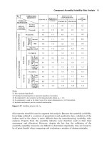
The Occurrence, Severity and Detectability Ratings are assessed on a scale of 1 to 10
and are illustrated in general terms in Figure 1.
Note, a comprehensive list of failure modes and causes of failure for mechanical
components is provided by Dieter (1986). These tables are particularly useful when
assessing the likely stress rupture failure mechanism for reliability work.
The Risk Priority Number (RPN) is the Occurrence (O), Severity (S) and Detect-
ability (D) ratings multiplied together:
RPN O Â S ÂD 1
This number should be used as a guide to the most serious problems, with the highest
numbers (typically greater than 100) requiring the most urgent action, particularly if
they have scored high Severity Ratings.
For more comprehensive FMEA Occurrence, Severity and Detectability Ratings,
see Figure 2. Note that Occurrence can be replaced by ®eld reliability data in the
form of failure rates scaled to the original ratings. This may be useful when assessing
product families or new designs based on existing ones.
Bene®ts
In the case of performing a design FMEA, the RPN score can:
. Highlight the need for design improvement
. Highlight priority areas for focusing limited resources
Figure 1
General ratings for FMEA Occurrence, Severity and Detectability
296 Appendix III
Figure 2
Typical FMEA ratings for Occurrence, Severity and Detectability
Appendix III 297
. Highlight the need for Statistical Process Control (SPC), 100% inspection, no
inspection
. Identify parts which have redundant function
. Prioritize those suppliers to which attention needs to be given
. Provide a basis for measures of performance.
Through its eective use, FMEA has been found to reduce:
. Customer complaints
. Late design changes
. Defects during manufacture and assembly
. Failures in the ®eld
. Failure costs (rework, warranty claims).
Key issues
. Can be used in product design or process development
. Must be management led and have a strategy of use
Figure 3
Design FMEA for a bicycle rear brake lever
298 Appendix III
. Training required to use analysis initially
. Initial resources committed minimal
. Team-based application essential
. Can be subjective
. Performed too late in product development in many cases
. Links well with Fault Tree Analysis (FTA) where possible causes of failure are
identi®ed
. Support design FMEAs with failure data wherever possible
. Input from the customer and suppliers is important
. Should be reviewed at regular stages
. Can help to build up a knowledge base for product families.
Example ± bicycle rear brake lever
The design FMEA process is shown in a case study on Figure 3. It highlights the areas
that need special attention, re¯ected in the highest Risk Priority Numbers, when
designing a bicycle rear brake lever. Using a Pareto chart, the RPN number, relating
to the relative risk of each failure mode, can be displayed as shown in Figure 4. The
analysis shows that design eort should be focused on the ¯exible element in the
assembly, i.e. the brake cable. This perhaps supports the personal experiences of
the reader, but the FMEA has shown this in a structured and rigorous appraisal of
the concept design.
250
200
150
100
50
0
RPN
POTENTIAL CAUSE OF FAILURE
PULL-OUT
FROM
NIPPLE
CABLE
SNAPS
PIVOT PIN
SHEARS
CLAMP
LOOSENS
LEVER
BREAKS
LEVER
BENDS
Figure 4
Pareto chart of RPN values against potential cause of failure for the rear brake lever design
Appendix III 299
Figure 5
Blank FMEA table
300 Appendix III
Figure 5 provides a blank table (complete with design revision section) used to
perform a design FMEA. It forms a traceable record of the design and its failure
modes and associated risks.
B. Quality Function Deployment (QFD)
(ASI, 1987; ASI, 1992; Clausing, 1994)
Description
In QFD customer requirements or `the voice of the customer' are cascaded down
through the product development process in four separate phases keeping the eort
focused on the important issues, linking customer requirements directly with actual
shop-¯oor operations/procedures.
In summary the objectives of QFD are to:
. Prioritize customer requirements and relate them to all stages of product develop-
ment
. Focus resources on the aspects of the product that are important for customer
satisfaction
. Provide a structured, team-driven product development process.
Placement in product development
QFD should be applied at the start of product development to help understand and
quantify customer requirements and support the de®nition of product requirements,
giving an overall picture of the requirements de®nition throughout the product
development process. Other tools and techniques can be used in conjunction with
it, for example Pareto chart, histogram, or data coming out of the FMEA can be
fed back at an early stage.
Application of the technique
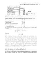
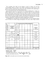
The four phases of QFD are described below and shown in Figure 6:
. Phase 1 ± Product Planning. Customer requirements from market research
information (including competitor analysis) and product speci®cation are
ranked in a matrix against the important design requirements, yielding a numerical
quanti®cation between the important customer requirements and product design
issues. The quanti®cation is performed by assessing whether the matrix elements
have either a weak, medium or strong relationship. Together with the importance
rating from the customer for a particular requirement, a points rating for the
design requirements is then determined. A popular convention for QFD Phase 1,
Appendix III 301
the product planning matrix, is shown in Figure 7. Critical design requirements
that are considered to be either new to a product, important by the customer or
dicult to produce are carried forward to the next phase.
. Phase 2 ± Design Deployment. The critical design requirements from Phase 1 (those
with a high points rating) are ranked with design characteristics where the relation-
ship between them is again quanti®ed, yielding important interface issues between
design and manufacture, for example those characteristics that require close
control during production. The critical design characteristics are then carried
forward to the next phase.
. Phase 3 ± Process Planning. The important design characteristics from Phase 2 are
ranked with key process operations, where quanti®cation yields actions to improve
the understanding of the processes involved and gain the necessary expertise early
on. The critical process operations highlighted are then carried forward to the next
phase.
. Phase 4 ± Production Planning. The critical process operations from Phase 3 are
ranked with production requirement issues, ultimately translating the important
customer requirements to production planning and establishing important actions
to be taken.
Bene®ts
The potential bene®ts of QFD are:
. Increased customer satisfaction
. Improved product quality
. Reduced design changes and associated costs
. Reduced lead times
. Improved documentation and traceability
. Promotes team working
Figure 6
The four phases of QFD (ASI, 1987)
302 Appendix III
Figure 7
QFD phase 1 matrix example for a toilet bleach container (ASI, 1992)
Appendix III 303
. Provides a structured approach to product development
. Improves customer/supplier relationship.
Key issues
. Can be used on products, software or services
. Must be management led and have an overall strategy for implementation and
application.
. Training required to use analysis initially
. Multi-disciplinary team-based application essential
. Can be subjective and tedious
. Organizations do not extend the use of QFD past the ®rst phase usually
. Involvement of customers and suppliers essential
. Review at regular intervals with customers and suppliers
. Identi®cation of customer requirements dicult sometimes
. Support QFD with existing data wherever possible
. Applied too late in many cases
. Can help to build up a knowledge base for product families.
Case study
An illustrative chart is shown in Figure 7, which relates to the design of a toilet bleach
container. It does not include all the customer wants. Figure 7 can be regarded as
Phase 1 product planning covering design requirements. The three remaining
phases are design deployment, process planning and production planning. Similar
charts are constructed for each of these phases (see Figure 6).
C. Design for Assembly/Design for Manufacture (DFA/
DFM)
(Boothroyd et al., 1994; CSC, 1995; Huang, 1996; Shimada et al., 1992)
Description
DFA/DFM is a team-based product design evaluation tool which, through simple
structured analysis, gives the information required by designers to achieve:
. Part count reduction
. Calculation of component manufacturing and assembly costs
. Ease of part handling
. Ease of assembly
. Ability to reproduce identically and without waste products which satisfy customer
requirements.
304 Appendix III
Placement in product development
DFA/DFM should be performed during concept design leading into the detailed
design stage to revise the product structure.
Application of the technique (CSC's DFA/MA methodology)
The analysis is carried out in four main stages (see Figure 8).
1. Functional analysis. The methodology enables each part to be classi®ed as
essential `A' parts or non-essential `B' parts. Given this awareness, redesigns can
be evolved around the essential components, from which reduced part count
normally results.
2. Manufacturing analysis. Component costs are calculated by considering materials,
manufacturing processes and aspects such as complexity, volume and tolerance.
This allows ideas for part count reduction to be tested since combining parts
can lead to more complex components and changes to manufacturing processes.
3. Handling analysis. Components must be correctly orientated before assembly can
take place. The diculty achieving this by either manual or mechanical means can
be assessed using the analysis. Components receiving high ratings should be
modi®ed to give an acceptable rating. Mistake proo®ng (or Poka Yoke) devices
Figure 8
DFA/MA ¯ow chart (CSC, 1995)
Appendix III 305
can be installed in the manufacturing and assembly processes to help ensure zero
defects.
4. Fitting analysis. For this to be possible, an assembly sequence plan must be
constructed and the diculty of assembling each part in the sequence rated using
the design for assembly analysis tables. Dicult assembly tasks and non-value
added processes are revealed as candidates for correction by redesign. Simple con-
cepts such as the ability to assemble in a layer fashion can result in major cost savings.
The assembly analysis stages 3 and 4 have the following measures of performance
which are accepted as an indication of good design:
. Functional analysis gives a Design Eciency Essential Parts/Total Parts !60%
. Handling analysis gives a Handling Ratio Total Ratings/Essential Parts 2.5
. Fitting analysis gives a Fitting Ratio Total Ratings/Essential Parts 2.5.
Bene®ts
The potential bene®ts of DFA/DFM are:
. Reduced part count
. Fewer parts means: improved reliability, fewer stock costs, fewer invoices from
fewer suppliers and possibly fewer quality problems
. Systematic component costing and process selection
. Improved yields
. Lower component and assembly costs
. Standardize components, assembly sequence and methods across product
`families' leading to improved reproducibility
. Faster product development and reduced time to market
. Lower level of engineering changes, modi®cations and concessions.
Typical results achieved by application of the DFA technique to date are approxi-
mately as follows:
. Parts count reduction 50%
. Assembly cost reduction 50%
. Product cost reduction 30%.
Key issues
. Must be management led
. Training required before use
. Resources consumed in product development can be signi®cant
. Team-based application and systematic approach is essential
. Many subjective analysis processes
. Manufacturing and technical feasibility of new component design solutions need
to be validated
. Early life failures are caused by latent defects.
306 Appendix III
Figure 9
DFA/MA trim screw example
Appendix III 307
Case study
A feasibility study aimed at automating the assembly of trim screws on a car headlight
design revealed diculties in handling the components and the assembly processes ±
complex assembly structure, complex access, turnover operation and automation
problems.
The trim screw assembly in its original form is shown in Figure 9(a). A product
improvement team used the DFA/MA methodology to analyse the design. The results
of the analysis are shown in the ®gure against a component list and a sequence of
assembly. Having analysed the existing trim screw design, certain undesirable
elements of the design were highlighted. This information together with original
conceptual changes to suit the proposed automation programme were used to
prompt a better design solution shown in Figure 9(b).
The number of parts in the redesign reduced from 5 to 2. A more simple product
structure and increased assembly design eciency resulted. Overall, component
and assembly costs were signi®cantly reduced. Figure 9(c) summarizes the results
of the analysis.
D. Design of Experiments (DOE)
(Grove and Davis, 1992; Kapur, 1993; Taguchi et al., 1989)
Description
DOE encompasses a range of techniques used to enable a business to understand the
eects of important variables in product and process development. It is normally used
when investigating a situation where there are several variables, one or more of which
may result in a problem either singly or in combination.
In summary the objectives of DOE are to:
. Identify causes of variation in critical product or process parameters
. Limit the eects of the variations identi®ed (where they can be controlled)
. Achieve reproducibility of best system performance in manufacture and use
. Optimize the product or process
. Reduce cost.
Placement in product development
QFD, FMEA and CA are useful in identifying critical characteristics early on in
product development and the results from these can be fed into DOE. DOE is
useful in investigating and validating these critical characteristics with respect to
technical requirements and their in¯uence on product and process quality.
308 Appendix III
Application of the technique
The systematic application of DOE should be based on three distinct phases:
Phase 1 ± Preparation. This is often referred to as the pre-experimental stage.
Experiments can take considerable time and resources, and good preparation is all
important. The results from other techniques are important inputs to this phase of
the methodology, providing focus and priority selection ®ltering. A summary of
the steps that should be considered is given below:
. De®ne the problem to be solved
. Agree the objectives and prepare a project plan
. Examine and understand the situation. Obtain and study all available data related
to the problem
. De®ne what needs to be measured to satisfy the project objectives
. Identify both the noise and factors to be controlled during the experiment and
select the levels to be considered. These should be representative of normal
operating range and suciently spaced to spot changes
. Establish an eective measuring system. Understand its variance and the likely
eects of this apparent variation in output.
Phase 2 ± Experimentation and analysis. Carrying out the planned trials and analytical
work will include the steps below:
. Select the techniques to be used. Decisions on the number of trials is invariably
coloured by cost, but always check they are balanced otherwise it may be false
economy
. Plan the trials. Consecutive trials should not aect each other
. Conduct the trials as planned. Results should be carefully recorded in a table or
machine along with any observations which may be regarded as potential errors
. Analysis and reporting of results, including a conformation run. The analysis of
results should be transparent. Simple approaches should be used where possible
to build con®dence and provide clarity.
Phase 3 ± Implementation. This phase is often called the post-experimental stage. It is
about acting on the results and communicating the lessons learnt. Some points on the
process are given below:
. Apply the ®ndings to resolve the problem
. Adopt a procedure for measuring and monitoring results such as SPC to detect
future changes that could in¯uence quality
. Communicate lessons learnt through the business and included in training
programmes.
Bene®ts
The potential bene®ts of DOE are:
. Improved product quality
Appendix III 309