System Analysis, Design, and Development Concepts, Principles, and Practices phần 8 pdf
Bạn đang xem bản rút gọn của tài liệu. Xem và tải ngay bản đầy đủ của tài liệu tại đây (2.71 MB, 84 trang )
47.3 Attributes of a Technical Decision 575
• Effectiveness Analysis “An analytical approach used to determine how well a system per-
forms in its intended utilization environment.” (Source: Kossiakoff and Sweet, System Engi-
neering, p. 448)
• Sanity Check “An approximate calculation or estimation for comparison with a result
obtained from a more complete and complex process. The differences in value should be rel-
atively small; if not, the results of the original process are suspect and further analysis is
required.” (Source: Kossiakoff and Sweet, System Engineering, p. 453)
• Suboptimization The preferential emphasis on the performance of a lower level entity at
the expense of overall system performance.
• System Optimization The act of adjusting the performance of individual elements of a
system to peak the maximum performance that can be achieved by the integrated set for a
given set of boundary conditions and constraints.
47.2 WHAT IS ANALYTICAL DECISION SUPPORT?
Before we begin our discussions of analytical decision support practices, we need to first under-
stand the context and anatomy of a technical decision. Decision support is a technical services
response to a contract or task commitment to gather, analyze, clarify, investigate, recommend, and
present fact-based, objective evidence. This enables decision makers to SELECT a proper (best)
course of action from a set of viable alternatives bounded by specific constraints—cost, schedule,
technical, technology, and support—and acceptable level of risk.
Analytical Decision Support Objective
The primary objective of analytical decision support is to respond to tasking or the need for tech-
nical analysis, demonstration, and data collection recommendations to support informed SE Process
Model decision making.
Expected Outcome of Analytical Decision Support
Decision support work products are identified by task objectives. Work products and quality records
include analyses, trade study reports (TSRs), and performance data. In support of these work prod-
ucts, decision support develops operational prototypes and proof of concept or technology demon-
strations, models and simulations, and mock-ups to provide data for supporting the analysis.
From a technical decision making perspective, decisions are substantiated by the facts of the
formal work products such as analyses and TSRs provided to the decision maker. The reality is that
the decision may have subconsciously been made by the decision maker long BEFORE the deliv-
ery of the formal work products for approval. This brings us to our next topic, attributes of tech-
nical decisions.
47.3 ATTRIBUTES OF A TECHNICAL DECISION
Every decision has several attributes you need to understand to be able to properly respond to the
task. The attributes you should understand are:
1. WHAT is the central issue or problem to be addressed?
2. WHAT is the scope of the task to be performed?
3. WHAT are the boundary constraints for the solution set?
Simpo PDF Merge and Split Unregistered Version -
576 Chapter 47 Analytical Decision Support
4. What is the degree of flexibility in the constraints?
5. Is the timing of the decision crucial?
6. WHO is the user of the decision?
7. HOW will the decision be used?
8. WHAT criteria are to be used in making the decision?
9. WHAT assumptions must be made to accomplish the decision?
10. WHAT accuracy and precision is required for the decision?
11. HOW is the decision is to be documented and delivered?
Scope the Problem to be Solved
Decisions represent approval of solutions intended to lead to actionable tasks that will resolve a
critical operational or technical or issue (COI/CTI). The analyst begins with understanding what:
1. Problem is to be solved.
2. Question is to be answered.
3. Issue is to be resolved.
Therefore, begin with a CLEAR and SUCCINCT problem statement.
Referral For more information about writing problem statements, refer to Chapter 14 on Under-
standing The Problem, Opportunity, and Solution Spaces concept.
If you are tasked to solve a technical problem and are not provided a documented tasking
statement, discuss it with the decision authority. Active listening enables analysts to verify their
understanding of the tasking. Add corrections based on the discussion and return a courtesy
copy to the decision maker. Then, when briefing the status of the task, ALWAYS include a restate-
ment of the task so ALL reviewers have a clear understanding of the analysis you were tasked to
perform.
Decision Boundary Condition Constraints and Flexibility
Technical decisions are bounded by cost, schedule, technology, and support constraints. In turn, the
constraints must be reconciled with an acceptable level of risk. Constraints sometimes are also
flexible. Talk with the decision maker and assess the amount of flexibility in the constraint. Docu-
ment the constraints and acceptable level of risk as part of the task statement.
Criticality of Timing of the Decision
Timing of decisions is CRUCIAL, not only from the perspective of the decision maker but also
that of the SE supporting the decision making. Be sensitive to the decision authority’s schedule and
the prevailing environment when the recommendations are presented. If the schedule is impracti-
cal, discuss it with the decision maker including level of risk.
Understand How the Decision Will Be Used and by Whom
Decisions often require approvals by multiple levels of organizational and customer stakeholder
decision makers. Avoid wasted effort trying to solve the wrong problem. Tactfully validate the deci-
sion problem statement by consensus of the stakeholders.
Simpo PDF Merge and Split Unregistered Version -
Document the Criteria for Decision Making
Once the problem statement is documented and the boundary constraints for the decision are estab-
lished, identify the threshold criteria that will be used to assess the success of the decision results.
Obtain stakeholder concurrence with the decision criteria. Make corrections as necessary to clarify
the criteria to avoid misinterpretation when the decision is presented for approval. If the decision
criteria are not documented “up front,” you may be subjected to the discretion of the decision maker
to determine when the task is complete.
Identify the Accuracy and Precision of the Analysis
Every technical decision involves data that have a level of accuracy and precision. Determine “up
front” what accuracy and precision will be required to support analytical results, and make sure
these are clearly communicated and understood by everyone participating. One of the worst things
analysts can do is discover after the fact that they need four-digit decimal data precision when they
only measured and recorded two-digit data. Some data collection exercises may not be repeatable
or practical. THINK and PLAN ahead: similar rules should be established for rounding data.
Author’s Note 47.1 As a reminder, two-digit precision data that require multiplication DO NOT
yield four-digit precision results; the best you can have is two-digit result due to the source data
precision.
Identify How the Decision Is to Be Delivered
Decisions need a point of closure or delivery. Identify what form and media the decision is to be
delivered: as a document, presentation, or both. In any case, make sure that your response is doc-
umented for the record via a cover letter or e-mail.
47.4 TYPES OF ENGINEERING ANALYSES
Engineering analyses cover a spectrum of disciplinary and specialty skills. The challenge for SEs
is to understand:
1. WHAT analyses may be required.
2. At WHAT level of detail.
3. WHAT tools are best suited for various analytical applications.
4. WHAT level of formality is required for documenting the results.
To illustrate a few of the many analyses that might be conducted, here’s a sample list.
• Mission operations and task analysis
• Environmental analysis
• Fault tree analysis (FTA)
• Finite element analysis (FEA)
• Mechanical analysis
• Electromagnetic interference (EMI)/electromagnetic countermeasures (EMC) analysis
• Optical analysis
• Reliability, availability, and maintainability (RAM) analysis
• Stress analysis
47.4 Types of Engineering Analyses 577
Simpo PDF Merge and Split Unregistered Version -
578 Chapter 47 Analytical Decision Support
• Survivability analysis
• Vulnerability analysis
• Thermal analysis
• Timing analysis
• System latency analysis
• Life cycle cost analysis
Guidepost 47.1 The application of various types of engineering analyses should focus on pro-
viding objective, fact-based data that support informed technical decision making. These results at
all levels aggregate into overall system performance that forms the basis of our next topic, system
performance evaluation and analysis.
47.5 SYSTEM PERFORMANCE EVALUATION AND ANALYSIS
System performance evaluation and analysis is the investigation, study, and operational analysis of
actual or predicted system performance relative to planned or required performance as documented
in performance or item development specifications. The analysis process requires the planning, con-
figuration, data collection, and post data analysis to thoroughly understand a system’s performance.
System Performance Analysis Tools and Methods
System performance evaluation and analysis employs a number of decision aid tools and methods
to collect data to support the analysis. These include models, simulations, prototypes, interviews,
surveys, and test markets.
Optimizing System Performance
System components at every level of abstraction inherently have statistical variations in physical
characteristics, reliability, and performance. Systems that involve humans involve statistical vari-
ability in knowledge and skill levels, and thus involve an element of uncertainty. The challenge
question for SEs is: WHAT combination of system configurations, conditions, human-machine tasks,
and associated levels of performance optimize system performance?
System optimization is a term relative to the stakeholder. Optimization criteria reflect the appro-
priate balance of cost, schedule, technical, technology, and support performance or combination
thereof.
Author’s Note 47.2 We should note here that optimization is for the total system. Avoid a con-
dition referred to as suboptimization unless there is a compelling reason.
Suboptimization
Suboptimization is a condition that exists when one element of a system—the PRODUCT, SUB-
SYSTEM, ASSEMBLY, SUBASSEMBLY, or PART level—is optimized at the expense of overall
system performance. During System Integration, Test, and Evaluation (SITE), system items at each
level of abstraction may be optimized. Theoretically, if the item is designed correctly, optimal per-
formance occurs at the planned midpoint of any adjustment ranges.
The underlying design philosophy here is that if the system is properly designed and compo-
nent statistical variations are validated, only minor adjustments may be required for an output to
Simpo PDF Merge and Split Unregistered Version -
47.6 Engineering Analysis Reports 579
be centered about some hypothetical mean value. If the variations have not been taken into account
or design modifications have been made, the output may be “off-set” from the mean value but
within its operating range when “optimized.” Thus, at higher levels of integration, this off-nominal
condition may impact overall system performance, especially if further adjustments beyond the
components adjustment range are required.
The Danger of Analysis Paralysis
Analyses serve as a powerful tool for understanding, predicting, and communicating system per-
formance. Analyses, however, cost money and consume valuable resources. The challenge ques-
tion for SEs to consider is, How GOOD is good enough? At what level or point in time does an
analysis meet minimal sufficiency criteria to be considered valid for decision making? Since engi-
neers, by nature, tend to immerse themselves in analytics, we sometimes suffer from a condition
referred to as “analysis paralysis.” So, what is analysis paralysis?
Analysis paralysis is a condition where an analyst becomes preoccupied or immersed in the
details of an analysis while failing to recognize the marginal utility of continual investigation. So,
HOW do SEs deal with this condition?
First, you need to learn to recognize the signs of this condition in yourself as well as others.
Although the condition varies with everyone, some are more prone than others. Second, aside from
personality characteristics, the condition may be a response mechanism to the work environment,
especially from paranoid, control freak managers who suffer from the condition themselves.
47.6 ENGINEERING ANALYSIS REPORTS
As a discipline requiring integrity in analytical, mathematical, and scientific data and computations
to support downstream or lower level decision making, engineering documentation is often sloppy
at best or simply nonexistent. One of the hallmarks of a professional discipline is an expectation
to document recommendations supported by factual, objective evidence derived empirically or by
observation.
Data that contribute to informed SE decisions are characterized by the assumptions, boundary
conditions, and constraints surrounding the data collection. While most engineers competently con-
sider relevant factors affecting a decision, the tendency is to avoid recording the results; they view
paperwork as unnecessary, bureaucratic documentation that does not add value directly to the deliv-
erable product. As a result, a professional, high-value analysis ends in mediocrity due to the analyst
lacking personal initiative to perform the task correctly.
To better appreciate the professional discipline required to document analyses properly, con-
sider a hypothetical visit to a physician:
EXAMPLE 47.1
You visit a medical doctor for a condition that requires several treatment appointments at three-month
intervals for a year. The doctor performs a high-value diagnosis and prescribes the treatments but fails to
record the medication and actions performed at each treatment event. At each subsequent treatment you and
the doctor have to reconstruct to the best of everyone’s knowledge the assumptions, dosages, and actions per-
formed. Aside from the medical and legal implications, can you imagine the frustration, foggy memories, and
“guesstimates” associated with these interactions. Engineering, as a professional discipline, is no different.
Subsequent decision making is highly dependent on the documented assumptions and constraints of previous
decisions.
Simpo PDF Merge and Split Unregistered Version -
The difference between mediocrity and high-quality professional results may be only a few minutes
to simply document critical considerations that yielded the analytical result and recommendations
presented. For SEs, this information should be recorded in an engineering laboratory notebook or
on-line in a network-based journal.
47.7 ENGINEERING REPORT FORMAT
Where practical and appropriate, engineering analyses should be documented in formal technical
reports. Contract or organizational command media sometimes specify the format of these reports.
If you are expected to formally report the results of an analysis and do not have specific format
requirements, consider the example outline below.
EXAMPLE 47.2
The following is an example of an outline that could be used to document a technical report.
1.0. INTRODUCTION
The introduction establishes the context and basis for the analysis. Opening statements identify the document,
its context and usage in the program, as well as the program this analysis is being performed to support.
1.1. Purpose
1.2. Scope
1.3. Objectives
1.4. Analyst/Team Members
1.5. Acronyms and Abbreviations
1.6. Definitions of Key Terms
2.0. REFERENCED DOCUMENTS
This section lists the documents referenced in other sections of the document. Note the operative title “Ref-
erenced Documents” as opposed to “Applicable Documents.”
3.0. EXECUTIVE SUMMARY
Summarize the results of the analysis such as findings, observations, conclusions, and recommendations: tell
them the bottom line “up front.” Then, if the reader desires to read about the details concerning HOW you
arrived at those results, they can do so in subsequent sections.
4.0. CONDUCT OF THE ANALYSIS
Informed decision making is heavily dependent on objective, fact based data. As such, the conditions under
which the analysis is performed must be established as a means of providing credibility for the results. Sub-
sections include:
4.1. Background
4.2. Assumptions
4.3. Methodology
4.4. Data Collection
4.5. Analytical Tools and Methods
4.6. Versions and Configurations
4.7. Statistical Analysis (if applicable)
4.8. Analysis Results
4.9. Observations
580 Chapter 47 Analytical Decision Support
Simpo PDF Merge and Split Unregistered Version -
4.10. Precision and Accuracy
4.11. Graphical Plots
4.12. Sources
5.0. FINDINGS, OBSERVATIONS, AND CONCLUSIONS
As with any scientific study, it is important for the analyst to communicate:
• WHAT they found.
• WHAT they observed.
• WHAT conclusions they derived from the findings and observations. Subsections include:
5.1. Findings
5.2. Observations
5.3. Conclusions
6.0. RECOMMENDATIONS
Based on the analyst’s findings, observations, and conclusions, Section 6.0 provides a set of prioritized rec-
ommendations to decision makers concerning the objectives established by the analysis tasking.
APPENDICES
Appendices provide areas to present supporting documentation collected during the analysis or that illustrates
how the author(s) arrived at their findings, conclusions, and recommendations.
Decision Documentation Formality
There are numerous ways to address the need to balance document decision making with time,
resource, and formality constraints. Approaches to document critical decisions range from a single
page of informal, handwritten notes to highly formal documents. Establish disciplinary standards
for yourself and your organization related to documenting decisions. Then, scale the documenta-
tion formality according to task constraints. Regardless of the approach used, the documentation
should CAPTURE the key attributes of a decision in sufficient detail to enable “downstream” under-
standing of the factors that resulted in the decision.
The credibility and integrity of an analysis often depends on who collected and analyzed the
data. Analysis report appendixes provide a means of organizing and preserving any supporting
vendor, test, simulation, or other data used by the analyst(s) to support the results. This is particu-
larly important if, at a later date, conditions that served as the basis for the initial analysis task
change, thereby creating a need to revisit the original analysis. Because of the changing conditions,
some data may have to be regenerated; some may not. For those data that have not changed, the
appendices minimize work on the new task analysis by avoiding the need to recollect or regener-
ate the data.
47.8 ANALYSIS LESSONS LEARNED
Once the performance analysis tasking and boundary conditions are established, the next step is to
conduct the analysis. Let’s explore some lessons learned you should consider in preparing to
conduct the analysis.
Lesson 1: Establish a Decision Development Methodology
Decision paths tend to veer off-course midway through the decision development process. Estab-
lish a decision making methodology “up front” to serve as a roadmap for keeping the effort on
47.8 Analysis Lessons Learned 581
Simpo PDF Merge and Split Unregistered Version -
track. When you establish the methodology “up front,” you have the visibility of clear, unbiased
THINKING unemcumbered by the adventures along the decision path. If you and your team are
convinced you have a good methodology, that plan will serve as a compass heading. This is not to
say that some conditions may warrant a change in methodology. Avoid changes unless there is a
compelling reason to change.
Lesson 2: Acquire Analysis Resources
As with any task, success is partially driven by simply having the RIGHT resources in place when
they are required. This includes:
1. Subject matter experts (SMEs)
2. Analytical tools
3. Access to personnel who may have relevant information concerning the analysis area
4. Analytical tools
5. Data that describe operating conditions and observations relevant to the analysis, and so
forth.
Lesson 3: Document Assumptions and Caveats
Every decision involves some level of assumptions and/or caveats. Document the assumptions in
a clear, concise manner. Make sure that the CAVEATS are documented on the same page as the
decision (footnotes, etc.) or recommendations. If the decision recommendations are copied or
removed from the document, the caveats will ALWAYS be in place. Otherwise, people may inten-
tionally or unintentionally apply the decision or recommendations out of context.
Lesson 4: Date the Decision Documentation
Every page of a decision document should marked indicating the document title, revision level,
date, page number, and classification level, if applicable. Using this approach, the reader can always
determine if the version they possess is current. Additionally, if a single page is copied, the source
is readily identifiable. Most people fail to perform this simple task. When multiple versions of a
report, especially drafts, are distributed without dates, the de facto version is determined by
WHERE the document is within a stack on someone’s desk.
Lesson 5: State the Facts as Objective Evidence
Technical reports must be based on the latest, factual information from credible and reliable
sources. Conjecture, hearsay, and personal opinions should be avoided. If requested, qualified opin-
ions can be presented informally with the delivery of the report.
Lesson 6: Cite Only Credible and Reliable Sources
Technical decisions often leverage and expand on existing knowledge and research, published or
verbal. If you use this information to support findings and conclusions, explicitly cite the source(s)
in explicit detail. Avoid vague references such as “read the [author’s] report” documented in an
obscure publication published 10 years ago that may be inaccessible or only available to the
author(s). If these sources are unavailable, quote passages with permission of the owner.
582
Chapter 47 Analytical Decision Support
Simpo PDF Merge and Split Unregistered Version -
47.9 Guiding Principles 583
Lesson 7: REFERENCE Documents versus
APPLICABLE Documents
Analyses often reference other documents and employ the terms APPLICABLE DOCUMENTS or
REFERENCED DOCUMENTS. People unknowingly interchange the terms. Using conventional
outline structures, Section 2.0 should be titled REFERENCED DOCUMENTS and list all sources
cited in the text. Other source or related reading material relevant to the subject matter is cited in
an ADDITIONAL READING section provided in the appendix.
Lesson 8: Cite Referenced Documents
When citing referenced documents, include the date and version containing data that serve as inputs
to the decision. People often believe that if they reference a document by title they have satisfied
analysis criteria. Technical decision making is only as good as the credibility and integrity of its
sources of objective, fact-based information. Source documents may be revised over time. Do your-
self and your team a favor: make sure that you clearly and concisely document the critical attrib-
utes of source documentation.
Lesson 9: Conduct SME Peer Reviews
Technical decisions are sometimes dead on arrival (DOA) due to poor assumptions, flawed deci-
sion criteria, and bad research. Plan for success by conducting an informal peer review by trusted
and qualified colleagues—the subject matter experts (SMEs)—of the evolving decision document.
Listen to their challenges and concerns. Are they highlighting critical operational and technical
issues (COIs/CTIs) that remain to be resolved, or overlooked variables and solutions that are
obscured by the analysis or research? We refer to this as “posturing for success” before the
presentation.
Lesson 10: Prepare Findings, Conclusions,
and Recommendations
There are a number of reasons as to WHY an analysis is conducted. In one case the technical deci-
sion maker may not possess current technical expertise or the ability to internalize and assimilate
data for a complex problem. So they seek out those who do posses this capability such as consult-
ants or organizations. In general, the analyst wants to know WHAT the subject matter experts
(SMEs) who are closest to the problems, issues, and technology suggest as recommenda-
tions regarding the decision. Therefore, analyses should include findings, recommendations, and
recommendations.
Based on the results of the analysis, the decision maker can choose to:
1. Ponder the findings and conclusions from their own perspective.
2. Accept or reject the recommendations as a means of arriving at an informed decision.
In any case, they need to know WHAT the subject matter experts (SMEs) have to offer regarding
the decision.
47.9 GUIDING PRINCIPLES
In summary, the preceding discussions provide the basis with which to establish the guiding prin-
ciples that govern analytical decision support practices.
Simpo PDF Merge and Split Unregistered Version -
Principle 47.1 Analysis results are only as VALID as their underlying assumptions, models, and
methodology. Validate and preserve their integrity.
47.10 SUMMARY
Our discussion of analysis decision support provided data and recommendations to support the SE Process
Model at all levels of abstraction. As an introductory discussion, analytical decision support employs various
tools addressed in the sections that follow:
• Statistical influences on SE decision making
• System performance analysis, budgets, and safety margins
• System reliability, availability, and maintainability
• System modeling and simulation
• Trade studies: analysis of alternatives
GENERAL EXERCISES
1. Answer each of the What You Should Learn from This Chapter questions identified in the Introduction.
2. Refer to the list of systems identified in Chapter 2. Based on a selection from the preceding chapter’s
General Exercises or a new system selection, apply your knowledge derived from this chapter’s topical
discussions. If you were the project engineer or Lead SE:
(a) What types of engineering analyses would you recommend?
(b) How would you collect data to support those analyses?
(c) Select one of the analyses. Write a simple analysis task statement based on the attributes of a
technical decision discussed at the beginning of this section.
ORGANIZATIONAL CENTRIC EXERCISES
1. Research your organization’s command media for guidance and direction concerning the implementation
of analytical decision support practices.
(a) What requirements are levied on programs and SEs concerning the conduct of analyses?
(b) Does the organization have a standard methodology for conducting an analysis? If so, report your
findings.
(c) Does the organization have a standard format for documenting analyses? If so, report your findings.
2. Contact small, medium and large contract programs within your organization.
(a) What analyses were performed on the program?
(b) How were the analyses documented?
(c) How was the analysis task communicated? Did the analysis report describe the objectives and scope
of the analysis?
(d) What level of formality—engineering notebook, informal report, or formal report—did technical
decision makers levy on the analysis?
(e) Were the analyses conducted without constraints or were they conducted to justify a predetermined
decision?
(f) What challenges or issues did the analysts encounter during the conduct of the analysis?
(g) Based on the program’s lessons learned, what recommendations do they offer as guidance for
conducting analyses on future programs?
584 Chapter 47 Analytical Decision Support
Simpo PDF Merge and Split Unregistered Version -
Additional Reading 585
3. Select two analysis reports from different contract programs.
(a) What is your assessment of each report?
(b) Did the program apply the right level of formality in documenting the analysis?
REFERENCES
IEEE Std 610.12-1990. 1990. IEEE Standard Glossary of
Modeling and Simulation Terminology. Institute of Elec-
trical and Electronic Engineers (IEEE). New York, NY.
Kossiakoff, Alexander, and Sweet, William N. 2003.
Systems Engineering Principles and Practice, New York:
Wiley-InterScience.
ADDITIONAL READING
ASD-100. 2004. National Airspace System System Engineering Manual, ATO Operations Planning. Washington, DC:
Federal Aviation Administration (FAA).
Simpo PDF Merge and Split Unregistered Version -
Chapter 48
Statistical Influences
on System Design
48.1 INTRODUCTION
For many engineers, system design evolves around abstract phrases such as “bound environmen-
tal data” and “receive data.” The challenge is: HOW do you quantify and bound the conditions for
a specific parameter? Then, how does an SE determine conditions such as:
1. Acceptable signal and noise (S/N) ratios?
2. Computational errors in processing the data?
3. Time variations required to process system data?
The reality is that the hypothetical boundary condition problems engineers studied in college aren’t
so ideal. Additionally, when a system or product is developed, multiple copies may produce varying
degrees of responses to a set of controlled inputs. So, how do SEs deal with the challenges of these
uncertainties?
Systems and products have varying degrees of stability, performance, and uncertainty that are
influenced by their unique form, fit, and function performance characteristics. Depending on the
price the User is willing to pay, we can improve and match material characteristics and processes
used to produce the SE systems and products. If we analyze a system’s or product’s performance
characteristics over a controlled range of inputs and conditions, we can statistically state the vari-
ance in terms of standard deviation.
This chapter provides an introductory overview of how statistical methods can be applied to
system design to improve capability performance. As a prerequisite to this discussion, you should
have basic familiarity with statistical methods and their applications.
What You Should Learn from This Chapter
1. How do you characterize random variations in system inputs sufficiently to bound the range?
2. How do SEs establish criteria for acceptable system inputs and outputs?
3. What is a design range?
4. How are upper and lower tolerance limits established for a design range?
5. How do SEs establish criteria for CAUTION and WARNING indicators?
6. What development methods can be employed to improve our understanding of the vari-
ability of engineering input data?
System Analysis, Design, and Development, by Charles S. Wasson
Copyright © 2006 by John Wiley & Sons, Inc.
586
Simpo PDF Merge and Split Unregistered Version -
48.2 Understanding the Variability of the Engineering Data 587
7. What is circular error probability (CEP)?
8. What is meant by the degree of correlation?
Definitions of Key Terms
• Circular Error Probability (CEP) The Gaussian probability density function (normal dis-
tribution) referenced to a central point with concentric rings representing the standard devi-
ations of data dispersion.
• Cumulative Error A measure of the total cumulative errors inherent within and created by
a system or product when processing statistically variant inputs to produce a standard output
or outcome.
• Logarithmic Distribution (Lognormal) An asymmetrical, graphical plot of the Poisson
probability density function depicting the dispersion and frequency of independent data
occurrences about a mean that is skewed from a median of the data distribution.
• Normal Distribution A graphical plot of the Gaussian probability density function depict-
ing the symmetrical dispersion and frequency of independent data occurrences about a central
mean.
• Variance (Statistical) “A measure of the degree of spread among a set of values; a measure
of the tendency of individual values to vary from the mean value. It is computed by subtract-
ing the mean value from each value, squaring each of these differences, summing these results,
and dividing this sum by the number of values in order to obtain the arithmetic mean of these
squares.” (Source: DSMC T&E Mgt. Guide, DoD Glossary of Test Terminology, p. B-21)
48.2 UNDERSTANDING THE VARIABILITY
OF THE ENGINEERING DATA
In an ideal world, engineering data are precisely linear or identically match predictive values with
zero error margins. In the real world, however, variations in mass properties and characteristics;
attenuation, propagation, and transmission delays; and human responses are among the uncertain-
ties that must be accounted for in engineering calculations. In general, the data are dispersed about
the mean of the frequency distribution.
Normal and Logarithmic Probability Density Functions
Statistically, we characterize the range dispersions about a central mean in terms of normal
(Gaussian) and logarithmic (Poisson) frequency distributions as shown in Figure 48.1.
Normal and logarithmic frequency distributions can be used to mathematically characterize
and bound engineering data related to statistical process control (SPC); queuing or waiting line
theory for customer service and message traffic; production lines; maintenance and repair, pressure
containment; temperature/humidity ranges; and so on.
Applying Statistical Distributions to Systems
In Chapter 3 What Is A System we characterized a system as having desirable and undesirable
inputs and producing desirable outputs. The system can also produce undesirable outputs—be they
electromagnetic, optical, chemical, thermal, or mechanical—that make the system vulnerable to
adversaries or create self-induced feedback that degrades system performance. The challenge for
SEs is bounding:
Simpo PDF Merge and Split Unregistered Version -
588 Chapter 48 Statistical Influences on System Design
1. The range of desirable or acceptable inputs and conditions from undesirable or unaccept-
able inputs.
2. The range of desirable or acceptable outputs and conditions from undesirable or unac-
ceptable outputs.
Recall Figure 3.2 of our discussion of system entity concepts where we illustrate the challenge in
SE Design decision making relative to acceptable and unacceptable inputs and outputs.
Design Input/Output Range Acceptability. Statistically we can bound and characterize the
range of acceptable inputs and outputs using the frequency distributions. As a simple example,
Figure 48.2 illustrates an example of a Normal Distribution that we can employ to characterize
input/output variability.
In this illustration we employ a Normal Distribution with a central mean. Depending on bound-
ing conditions imposed by the system application, SEs determine the acceptable design range that
includes upper and lower limits relative to the mean.
Range of Acceptable System Performance. During normal system operations, system or
product capabilities perform within an acceptable (Normal) Design Range. The challenge for
SEs is determining WHAT the thresholds for alerting system operators and maintainers
WHEN system performance is OFF nominal and begins to pose a risk or threat to the operators,
EQUIPMENT, public, or environment. To better understand this point, let’s examine it using
Figure 48.2.
In the figure we have a Normal Distribution about a central mean and characterized by four
types of operating ranges:
• DESIGN Range The range of engineering parameter values for a specific capability and con-
ditions that bound the ACCEPTABLE upper and lower tolerance limits.
• NORMAL Operating Range The range of acceptable engineering parameter values for a
specific capability within the design range that clearly indicates capability performance under
a given set of conditions is operating as expected and does not pose a risk or threat to the oper-
ators, EQUIPMENT, general public, or environment.
• CAUTIONARY Range The range of engineering parameter values for a specific capabil-
ity that clearly indicates capability performance under a given set of conditions is beyond or
Normal Distribution
(Gaussian)
Logarithmic Distribution
(Poisson)
Mean/Median
Mean
-
•
+
•
-
•
+
•
Median
Figure 48.1 Basic Types of Statistical Frequency Distributions
Simpo PDF Merge and Split Unregistered Version -
48.2 Understanding the Variability of the Engineering Data 589
OUTSIDE the Normal Operating Range and potentially poses a risk or threat to the opera-
tors, EQUIPMENT, general public, or environment.
• WARNING Range The range of engineering parameter values for a specific capability and
conditions that clearly poses a high level of risk or a threat to the operators, EQUIPMENT,
public, or environment with catastrophic consequences.
This presents several decision-making challenges for SEs:
1. What is the acceptable Design Range that includes upper and lower Caution Ranges?
2. WHAT are the UPPER and LOWER limits and conditions of the acceptable Normal
Operating Range?
3. WHAT are the thresholds and conditions for the WARNING Range?
4. WHAT upper and lower Design Safety Margins and conditions must be established for the
system relative to the Normal Operating Range, Caution Range, and Warning Range?
These questions, which are application dependent, are typically difficult to answer. Also keep in
mind that this graphic reflects a single measure of performance (MOP) for one system entity at a
specific level of abstraction. The significance of this decision is exacerbated by the need to allo-
cate the design range to lower level entities, which also have comparable performance distribu-
tions, ranges, and safety margins. Obviously, this poses a number of risks. For large, complex
systems, HOW do we deal with this challenge?
There are several approaches for supporting the design thresholds and conditions.
First, you can model and simulate the system and employ Monte Carlo techniques to assess
the most likely or probable outcomes for a given set of use case scenarios. Second, you can lever-
age modeling and simulation results and develop a prototype of the system for further analysis and
Normal
Operating Range
Design Nominal (Mean)
Design Lower
Limit (LL)
Design Upper
Limit (UL)
Design Range
Cautionary Range
Warning Range
Lower Toleranc e Upper Tolerance
? ?
Lower Design
Safety Margin
(Application
Dependent)
Upper Design
Safety Margin
(Application
Dependent)
Figure 48.2 Application Dependent Normalized Range of Acceptable Operating Condition Limits
Simpo PDF Merge and Split Unregistered Version -
590 Chapter 48 Statistical Influences on System Design
evaluation. Third, you can employ spiral development to evolve a set of requirements over a set of
sequential prototypes.
Now let’s shift our focus to understanding how statistical methods apply to system
development.
48.3 STATISTICAL METHOD APPLICATIONS
TO SYSTEM DEVELOPMENT
Statistical methods are employed throughout the System Development Phase by various disciplines.
For SEs, statistical challenges occur in two key areas:
1. Bounding specification requirements.
2. Verifying specification requirements.
Statistical Challenges in Writing Specification Requirements
During specification requirements development, Acquirer SEs are challenged to specify the accept-
able and unacceptable ranges of inputs and outputs for performance-based specifications. Consider
the following example:
EXAMPLE 48.1
Under specified operating conditions, the Sensor System shall have a probability of detection of 0.XX over a
(magnitude) spectral frequency range.
Once the contract is awarded, System Developer SEs are challenged to determine, allocate, and
flow down system performance budgets and safety margins requirements derived from higher level
requirements such as in the example above. The challenge is analyzing the example above to derive
requirements for PRODUCT, SUBSYSTEM, ASSEMBLY, and other levels. Consider the follow-
ing example.
EXAMPLE 48.2
The (name) output shall have a ±3s worst-case error of 0.XX for Input Parameter A distributions between
0.000 vdc to 10.000 vdc.
Statistical Challenges in Verifying Specification Requirements
Now let’s suppose that an SE’s mission is to verify the requirement stated in Example 48.2. For
simplicity, let’s assume that the sampled end points of Input data are 0.000 vdc and 10.000vdc with
a couple of points in between. We collect data measurements as a function of Input Data and plot
them. Panel A of Figure 48.3 might be representative of thess data.
Applying statistical methods, we determine the trend line and ±3s boundary conditions based
on the requirement. Panels C and D of Figure 48.3 could represent these data. Then we super-
impose the trend line and ±3s boundaries and verify that all system performance data are within
the acceptable range indicating the system passed (Panel D).
Simpo PDF Merge and Split Unregistered Version -
48.5 Cumulative System Performance Effects 591
48.4 UNDERSTANDING TEST DATA DISPERSION
The preceding discussion focuses on design decisions. Let’s explore how system analysts and SEs
statistically deal with test data that may be used as an input into SE design decision making or ver-
ifying that a System Performance Specification (SPS) or item development specification require-
ments has been achieved.
Suppose that we conduct a test to measure system or entity performance over a range of input
data as shown in Panel A of Figure 48.3. As illustrated, we have a number of data points that have
a positive slope. This graphic has two important aspects:
1. Upward sloping trend of data
2. A dispersion of data along the trend line.
In this example, if we performed a Least Squares mathematical fit of the data, we could establish
the slope and intercepts of the trend line using a simple y = mx + b construct.
Using the trend line as a central mean for the data set as a function of Input Data (X-axis), we
find that the corresponding Y data points are dispersed about the mean as illustrated in Panel C.
Based on the standard deviation of the data set, we could say that there is 0.9973 probability that
a given data point lies within the ±3s about the mean. Thus, Panel D depicts the results of pro-
jecting the ±3s lines along the trend line.
48.5 CUMULATIVE SYSTEM PERFORMANCE EFFECTS
Our discussions to this point focus on statistical distributions relative to a specific capability param-
eter. The question is: HOW do these errors propagate throughout the system? There are several
factors that contribute to the error propagation:
3
Data Dispersion
Measured
Performance
Data
Input Data
Data
Dispersion
Data
Dispersion
Measured
P
erformance
Data
Measured
P
erformance
Data
Input Data Input Data
A
B
C D
+3
s
-3
s
+3
s
-3
s
Figure 48.3 Understanding Engineering Data Dispersion
Simpo PDF Merge and Split Unregistered Version -
592 Chapter 48 Statistical Influences on System Design
1. OPERATING ENVIRONMENT influences on system component properties.
2. Timing variations.
3. Computational precision and accuracy.
4. Drift or aliasing errors as a function of time.
From a total system perspective, we refer to this concept as cumulative error. Figure 48.4 provides
an example.
Let’s assume we have a simple system that computes the difference between two parameters
A and B. If we examine the characteristics of parameters A and B, we find that each parameter has
different data dispersions about its predicted mean.
Ultimately, if we intend to compute the difference between parameter A and parameter B, both
parameters have to be scaled relative to some normalized value. Otherwise, we get an “apples and
oranges” comparison. So, we scale each input and make any correctional offset adjustments. This
simply solves the functional aspect of the computation. Now, what about errors originating from
the source values about a nominal mean plus all intervening scaling operations? The answer is:
SEs have to account for the cumulative error distributions related to errors and dispersions. Once
the system is developed, integrated, and tested, SYSTEM Level optimization is used to correct for
any errors and dispersions.
48.6 CIRCULAR ERROR PROBABILITY (CEP)
The preceding discussion focused on analyzing and allocating system performance within the
system. The ultimate test for SE decision making comes from the actual field results. The question
is: How do cumulative error probabilities impact overall operational and system effectiveness?
Perhaps the best way to answer this question is a “bull’s-eye target” analogy using Figure 48.5.
Design
Lower Limit
Design
Upper Limit
Design
Nominal
Parameter
Scaling
Parameter
Scaling
Scaled
Difference
Scaled
Difference
Parameter
Scaling
Parameter
Scaling
Compensation
Adjustments
• Offset
• Amplitude
• Range Filtering
Compensation
Adjustments
• Offset
• Amplitude
• Range Filtering
Compensation
Adjustments
• Offset
• Amplitude
• Range Filtering
Compensation
Adjustments
• Offset
• Amplitude
• Range Filtering
2
1
3
4
5
6 7
8
9
10
Figure 48.4 Understanding Cumulative Error Statistics
Simpo PDF Merge and Split Unregistered Version -
48.6 Circular Error Probability (CEP) 593
Our discussions up to this point have focused on the dispersion of data along linear trend lines
with a central mean. There are system applications whereby data are dispersed about a central point
such as the “bull’s eye” illustrated in Figure 48.5. In these cases the ±1s, ±2s, and ±3s points lie
on concentric circles aligned about a central mean located at the bull’s eye. Applications of this
type are generally target based such as munitions, firearms, and financial plans. Consider the fol-
lowing example:
EXAMPLE 48.3
Suppose that you conduct an evaluation of two competing rifle systems, System A and System B. We will
assume statistical sampling methods are employed to determine a statistically valid sample size. Specification
requirements state that 95% of the shots must be contained within circle with a diameter of X inches centered
at the bull’s eye.
Each system is placed in a test fixture and calibrated. When environmental conditions are accept-
able, expert marksmen “live fire” the required number of rounds from each rifle. Marksmen
are unaware of the manufacturer of each rifle. Miss distance firing results are shown in Panels A
and B.
Using the theoretical crosshair as the origin, you superimpose the concentric lines about the
bull’s eye representing the ±1s, ±2s, and ±3s points as illustrated in the center of the graphic.
Panels C and D depict the results with miss distance as the deciding factor, System B is superior.
In this simple, ideal example we focused exclusively on system effectiveness, not cost effec-
tiveness, which includes system effectiveness. The challenge is: things are not always ideal and
rifles are not identical in cost. What do you do? The solution lies in the Cost as an Independent
Variable (CAIV) and trade study utility function concepts discussed earlier in Figure 6.1. What is
the utility function of the field performance test results relative to cost and other factors?
1
A
System A
B
System B
1s
2s
3s
C
System A
Dispersion
D
System B
Dispersion
-3s -2s -1s +1s +2s +3s
Drawing Not to Scale
Figure 48.5 Circular Error Probability Example
Simpo PDF Merge and Split Unregistered Version -
594 Chapter 48 Statistical Influences on System Design
x
y
Positive Correlation
x
y
Negative Correlation
x
y
Data variance
convergence toward
r=+1
Positive Correlation
Convergence
x
y
Negative Correlation
Convergence
Data variance
convergence toward
r=–1
x
y
Data Variance Correlation
Converging Toward r=0
Positive Correlation
r=+1
Negative Correlation
r=–1
Where:
r = Correlation Coefficient
A B C
No Correlation
D E
Figure 48.6 Understanding Data Correlation
If System A costs one-half as much as System B, does the increased performance of System
B substantiate the cost? You may decide that the ±3s point is the minimum threshold requirement
for system acceptability. Thus, from a CAIV perspective, System A meets the specification thresh-
old requirement and costs one-half as much, yielding the best value.
You can continue this analysis further by evaluating the utility of hitting the target on the first
shot for a given set of time constraints, and so forth.
48.7 DATA CORRELATION
Engineering often requires developing mathematical algorithms that model best-fit approximations
to real world data set characterizations. Data are collected to validate that a system produces high-
quality data within predictable values. We refer to the degree of “fit” of the actual data to the stan-
dard or approximation as data correlation.
Data correlation is a measure of the degree to which actual data regress toward a central mean
of predicted values. When actual values match predicted values, data correlation is 1.0. Thus, as
data set variances diverge away from the mean trend line, the degree of correlation represented by
r, the correlation coefficient, diminishes toward zero. To illustrate the concept of data correlation
and convergence, Figure 48.6 provides examples.
Positive and Negative Correlation
Data correlation is characterized as positive or negative depending on the SLOPE of the line rep-
resenting the mean of the data set over a range of input values. Panel A of Figure 48.6 represents
a positive (slope) correlation; Panel B represents a negative (slope) correlation. This brings us to
our next point, convergence or regression toward the mean.
Simpo PDF Merge and Split Unregistered Version -
Organizational Centric Exercises 595
Regression toward Convergence
Since engineering data are subject to variations in physical characteristics, actual data do not always
perfectly match the predicted values. In an ideal situation we could state that the data correlate
over a bounded range IF all of the values of the data set are perfectly aligned on the mean trend
line as illustrated in Panels A and B of Figure 48.6.
In reality, data are typically dispersed along the trend line representing the mean values. Thus,
we refer to the convergence or data variance toward the mean as the degree of correlation. As data
sets regress toward a central mean, the data variance or correlation increases toward r =+1 or
-1 as illustrated in Panels D and E. Data variances that decrease toward r = 0 indicate decreasing
convergence or low correlation. Therefore, we characterize the relationship between data parame-
ters as positive or negative data variance convergence or correlation.
48.8 SUMMARY
Our discussions of statistical influences on system design practices were predicated on a basic understanding
of statistical methods and provided a high-level overview of key statistical concepts that influence SE design
decisions.
We highlighted the importance of using statistical methods to define acceptable or desirable design ranges
for input and output data. We also addressed the importance of establishing boundary conditions for NORMAL
operating ranges, CAUTIONARY ranges, WARNING ranges, as well as establishing safety margins. Using
the basic concepts as a foundation, we addressed the concept of cumulative errors, circular error probabili-
ties (CEP), and data correlation. We also addressed the need to bound acceptable or desirable system outputs
that include products, by-products, and services.
Statistical data variances have significant influence on SE technical decisions such as system perform-
ance, budgets, and safety margins and operational and system effectiveness. What is important is that SEs:
1. Learn to recognize and appreciate engineering input/output data variances
2. Know WHEN and HOW to apply statistical methods to understand SYSTEM interactions with its
OPERATING ENVIRONMENT.
GENERAL EXERCISES
1. Answer each of the What You Should Learn from This Chapter questions identified in the Introduction.
2. Refer to the list of systems identified in Chapter 2. Based on a selection from the preceding chapter’s
General Exercises or a new system, selection, apply your knowledge derived from this chapter’s topical
discussions. Specifically identify the following:
(a) What inputs of the system can be represented by statistical distributions?
(b) How would you translate those inputs into a set of input requirements?
(c) Based on processing of those inputs, do errors accumulate and, if so, what is the impact?
(d) How would you specify requirements to minimize the impacts of errors?
ORGANIZATIONAL CENTRIC EXERCISES
1. Contact a technical program in your organization. Research how the program SEs accommodated statisti-
cal variability for the following:
(a) Acceptable data input and output ranges for system processing
(b) External data and timing variability
Simpo PDF Merge and Split Unregistered Version -
596 Chapter 48 Statistical Influences on System Design
2. For systems that require performance monitoring equipment such as gages, meters, audible warnings,
and flashing lights, research how SEs determined threshold values for activating the notifications or
indications.
REFERENCE
Defense Systems Management College (DSMC). 1998. DSMC Test and Evaluation Management Guide, 3rd ed. Defense
Acquisition Press. Ft. Belvoir, VA.
ADDITIONAL READING
Blanchard, Benjamin S., and J. Fabrycky, Wolter.
1990. Systems Engineering and Analysis, 2nd ed. Engle-
wood Cliff, NJ: Prentice-Hall.
Langford, John W. 1995. Logistics: Principles and Appli-
cations. New York: McGraw-Hill.
National Aeronautics and Space Administration (NASA).
1994. Systems Engineering “Toolbox” for Design-
Oriented Engineers. NASA Reference Publication 1358.
Washington, DC.
Simpo PDF Merge and Split Unregistered Version -
Chapter 49
System Performance Analysis,
Budgets, and Safety Margins
49.1 INTRODUCTION
System effectiveness manifests itself via the cumulative performance results of the integrated set of
System Elements at a specific instance in time. That performance ultimately determines mission
and system objectives success—in some cases, survival.
When SEs allocate system performance, there is a tendency to think of those requirements as
static parameters—for example, “shall be +12.3 ± 0.10vdc.” Aside from status switch settings or
configuration parameters, seldom are parameters static or steady state.
From an SE perspective, SEs partition and organize requirements via a hierarchical framework.
Take the example of static weight. We have a budget of 100 pounds to allocate equally to three
components. Static parameters make the SE requirements allocation task a lot easier. This is not
the case for many system requirements. How do we establish values for system inputs that are
subject to variations such as environmental conditions, time of day, time of year, signal properties,
human error and other variables?
System requirement parameters are often characterized by statistical value distributions—such
as Normal (Gaussian), Binomial, and LogNormal (Poisson)—with frequencies and tendencies about
a mean value. Using our static requirements example above, we can state that the voltage must be
constrained to a range of +12.20vdc (-3s) to +12.40 vdc (+3s) with a mean of +12.30 vdc for a
prescribed set of operating conditions.
On the surface, this sounds very simple and straightforward. The challenge is: How did SEs
decide:
1. That the mean value needed to be +12.30 vdc?
2. That the variations could not exceed 0.10 vdc?
This simple example illustrates one of the most challenging and perplexing aspects of System Engi-
neering—allocating dynamic parameters.
Many times SEs simply do not have any precedent data. For example, consider human attempts
to build bridges, develop and fly an aircraft, launch rockets and missiles, and land on the Moon
and Mars. Analysis with a lot of trial and error data collection and observation may be all you
have to establish initial estimates of these parameters.
There are a number of ways one can determine these values. Examples include:
System Analysis, Design, and Development, by Charles S. Wasson
Copyright © 2006 by John Wiley & Sons, Inc.
597
Simpo PDF Merge and Split Unregistered Version -
1. Educated guesses based on seasoned experience.
2. Theoretical and empirical trial and error analysis.
3. Modeling and simulation with increasing fidelity.
4. Prototyping demonstrations.
The challenge is being able to identify a reliable, low-risk, level of confidence method of deter-
mining values for statistically variant parameters.
This chapter describes how we allocate System Performance Specification (SPS) requirements
to lower levels. We explore how functional and nonfunctional performance are analyzed and allo-
cated. This requires building on previous practices such as statistical influences on system design
discussed in the preceding chapter. We introduce the concepts of decomposing cycle time based
performances into queue, process, and transport times. Finally, we conclude by illustrating how
performance budgets and safety margins enable us to achieve SPS performance requirements.
What You Should Learn from This Chapter
1. What is system performance analysis?
2. What is a cycle time?
3. What is a queue time?
4. What is a transport time?
5. What is a processing time?
6. What is a performance budget?
7. How do you establish performance budgets?
8. What is a safety margin?
Definitions of Key Terms
• “Design-to” MOP A targeted mean value bounded by minimum and/or maximum thresh-
old values levied on a system capability performance parameter to constrain decision
making.
• Performance Budget Allocation A minimum, maximum, or min-max constraint that repre-
sents the absolute thresholds that bound a capability or performance characteristic.
• Processing Time The statistical mean time and tolerance that statistically characterizes the
time interval between an input stimulus or cue event and the completion of processing of
the input(s).
• Queue Time The statistical mean time and tolerance that characterizes the time interval
between the arrival of an input for processing and the point where processing begins.
• Safety Margin A portion of an assigned capability or physical characteristic measure of
performance (MOP) that is restricted from casual usage to cover instances in which the bud-
geted performance exceeds its allocated MOP.
• System Latency The time differential between a stimulus or cue events and a system
response event. Some people refer to this as the responsivity of the system for a specific
parameter.
• Transport Time The statistical mean time and tolerance that characterizes the time inter-
val between transmission of an output and its receipt at the next processing task.
598
Chapter 49 System Performance Analysis, Budgets, and Safety Margins
Simpo PDF Merge and Split Unregistered Version -
49.2 PERFORMANCE “DESIGN-TO”
BUDGETS AND SAFETY MARGINS
Every functional capability or physical characteristic of a system or item must be bounded by per-
formance constraints. This is very important in top-down/bottom-up/horizontal design whereby
system functional capabilities are decomposed, allocated, and flowed down into multiple levels of
design detail.
Achieving Measures of Performance (MOPs)
The mechanism for decomposing system performance into subsequent levels of detail is referred
to as performance budgets and margins. In general, performance budgets and margins allow SEs
to impose performance constraints on functional capabilities that include a margin of safety. Philo-
sophically, if overall system performance must be controlled, so should the contributing entities at
multiple levels of abstraction.
Performance constraints are further partitioned into: 1) “design-to” measures of performance
(MOPs) and 2) performance safety margins.
Design-to MOPs
Design-to MOPs serve as the key mechanism for allocating, flowing down, and communicating
performance constraints to lower levels system items. The actual allocation process is accom-
plished by a number of methods ranging from equitable shares to specific allocations based on arbi-
trary and discretionary decisions or decisions supported by design support analyses and trade
studies.
Safety Margins
Safety margins accomplish two things. First, they provide a means to accommodate variations in
tolerances, accuracies, and latencies in system responses plus errors in human judgment. Second,
they provide a reserve for decision makers to trade off misappropriated performance inequities as
a means of optimizing overall system performance.
Performance safety margins serve as contingency reserves to compensate for component vari-
ations or to accommodate worst-case scenarios that:
1. Could have been underestimated.
2. Potentially create safety risks and hazards.
3. Result from human errors in computational precision and accuracy.
4. Are due to physical variations in materials properties and components
5. Result from the “unknowns.”
Every engineering discipline employs rules of thumb and guidelines for accommodating safety
margins. Typically, safety margins might vary from 5% to 200% on average, depending on the
application and risk.
There are limitations to the practicality of safety margins in terms of: 1) cost–benefits, 2) prob-
ability or likelihood of occurrence, 3) alternative actions, and 4) reasonable measures, among other
things. In some cases, the implicit cost of increasing safety margin MOPs above a practical level can
be offset by taking appropriate system or product safety precautions, safeguards, markings, and pro-
cedures that reduce the probability of occurrence.
49.2 Performance “Design-to” Budgets and Safety Margins 599
Simpo PDF Merge and Split Unregistered Version -