Engineering Materials 2E VOLUME1 Episode 2 ppsx
Bạn đang xem bản rút gọn của tài liệu. Xem và tải ngay bản đầy đủ của tài liệu tại đây (999.11 KB, 25 trang )
The price and availability
of
materials
17
COPPER
199W
RUBBER
199W
Fig.
2.1.
The
fluctuations in price
of
copper and
of
rubber between September 1993 and May 1994.
diamonds today is partly caused by a flood of both from Russia since the end of the
Cold War.
The long-term changes are of a different kind. They reflect, in part, the real cost (in
capital investment, labour and energy) of extracting and transporting the ore or
feedstock and processing it to give the engineering material. Inflation and increased
energy costs obviously drive the price up;
so,
too, does the necessity to extract
materials, like copper, from increasingly lean ores; the leaner the ore, the more
machinery and energy are required to crush the rock containing it, and to concentrate
it to the level that the metal can be extracted.
In the long term, then, it is important to know which materials are basically plentiful,
and which are likely to become scarce. It is also important to know the extent of our
dependence on materials.
The use-paitern
of
materials
The way in which materials are used in a developed nation is fairly standard. All
consume steel, concrete and wood in construction; steel and aluminium in general
engineering; copper in electrical conductors; polymers in appliances, and so forth; and
roughly in the same proportions. Among metals, steel
is
used in the greatest quantities
by far:
90%
of all the metal produced in the world is steel. But the non-metals wood and
concrete beat steel
-
they are used in even greater volume.
About
20%
of the total import bill of a country like Britain is spent on engineering
materials. Table
2.2
shows how this spend is distributed. Iron and steel, and the raw
materials used to make them, account for about a quarter of it. Next are wood and
lumber
-
still widely used in light construction. More than a quarter is spent on the
metals copper, silver, aluminium and nickel. All polymers taken together, including
rubber, account for little more than
10%.
If
we include the further metals zinc, lead, tin,
tungsten and mercury, the list accounts for
99%
of all the money spent abroad on
materials, and we can safely ignore the contribution of materials which do not appear
on it.
18
Engineering Materials
1
Table
2.2
UK
imports of engineering materials, raw and
semis: Percentage
of
total cost
Iron and steel
Wood
and lumber
Copper
Plastics
Silver and platinum
Aluminium
Rubber
Nickel
Zinc
Lead
Tin
Pulp/paper
Glass
Tungsten
Mercury
Etc.
27
21
13
9.7
6.5
5.4
5.1
2.7
2.4
2.2
1.6
1.1
0.8
0.3
0.2
1
.o
Ubiquitous materials
The
composition
of
the
earth’s
crust
Let
us
now shift attention from what we
use
to what is widely
available.
A
few
engineering materials are synthesised from compounds found in the earths oceans and
atmosphere: magnesium is an example. Most, however, are won by mining their ore
from the earth‘s crust, and concentrating it sufficiently to allow the material to be
extracted or synthesised from it. How plentiful and widespread are these materials on
which we depend
so
heavily? How much copper, silver, tungsten, tin and mercury in
useful concentrations does the crust contain? All five are rare: workable deposits of
them are relatively small, and are
so
highly localised that many governments classify
them as of strategic importance, and stockpile them.
Not all materials are
so
thinly spread. Table
2.3
shows the relative abundance of the
commoner elements in the earth’s crust. The crust is
47%
oxygen by weight or
-
because oxygen is a big atom, it occupies
96%
of the volume (geologists are fond of
saying that the earths crust is solid oxygen containing a few per cent of impurities).
Next in abundance are the elements silicon and aluminium; by far the most plentiful
solid materials available to
us
are silicates and alumino-silicates.
A
few metals appear
on the list, among them iron and aluminium both of which feature also in the list of
widely-used materials. The list extends as far as carbon because it is the backbone of
virtually all polymers, including wood. Overall, then, oxygen and its compounds are
overwhelmingly plentiful
-
on every hand we are surrounded by oxide-ceramics, or the
raw materials to make them. Some materials are widespread, notably iron and
aluminium; but even for these the local concentration is frequently small, usually too
small
to
make it economic to extract them. In fact, the raw materials for making
polymers are more readily available at present than those for most metals. There are
The
price and availability
of
materials
19
Table
2.3
Abundance
of
elements/weight percent
Oceans
Atmosphere
Oxygen
Silicon
Aluminium
Iron
Calcium
Sodium
Potassium
Magnesium
Titanium
Hydrogen
Phosphorus
Manganese
Fluorine
Barium
Strontium
Sulphur
Carbon
47
27
8
5
4
3
3
2
0.4
0.1
0.1
0.1
0.06
0.04
0.04
0.03
0.02
oxygen
85
Nitrogen
79
Chlorine
2
Argon
2
Magnesium
0.1
Sulphur
0.1
Hydrogen
10
oxygen
19
Sodium
1
Carbon dioxide
0.04
Calcium
0.04
Potassium
0.04
Bromine
0.007
Carbon
0.002
The total mass
of
the crust
to
a
depth
of
1
km
is
3
x
IO2’
kg; the mass
of
the Oceans
is
IO2’
kg;
ht
of the
atmosphere
is
5
x
1018
kg.
huge deposits of carbon in the earth: on a world scale, we extract
a
greater tonnage of
carbon every month than we extract iron in a year, but at present we simply burn it.
And the second ingredient of most polymers
-
hydrogen
-
is also one of the most
plentiful of elements. Some materials
-
iron, aluminium,
silicon,
the elements
to
make
glass and cement
-
are plentiful and widely available. But others
-
mercury, silver,
tungsten are examples
-
are scarce and highly localised, and
-
if the current pattern of
use continues
-
may not last very long.
Exponential growth and consumption doubling-time
How do we calculate the lifetime of a resource like mercury? Like almost all materials,
mercury is being consumed at a rate which is growing exponentially with time (Fig.
2.2),
simply because both population and living standards grow exponentially. We
analyse this in the following way. If the current rate of consumption in tonnes per year
is
C
then exponential growth means that
dC
r
dt
100
-c
_-
-
(2.1)
where, for the generally small growth rates we deal with here
(1
to
5%
per year),
r
can
be thought of as the percentage fractional rate of growth per year. Integrating gives
20
Engineering
Materials
1
to
Time
t
(year)
Fig.
2.2.
The exponentially rising consumption
of
materials.
r
-C
100
(2.2)
where
Co
is the consumption rate at time
t
=
to.
The
doubIing-time
tD
of consumption is
given by setting
C/Co
=
2
to give
Steel consumption is growing at less than
2%
per year
-
it doubles about every 35 years.
Polymer consumption is rising at about
5%
per year
-
it doubles every
14
years. During
times of boom
-
the
1%Os
and
1970s
for instance
-
polymer production increased much
faster than this, peaking at
18%
per year (it doubled every
4
years), but it has now fallen
back to a more modest rate.
Resource
availability
The availability of a resource depends on the degree to which it is
locdised
in one or
a
few countries (making it susceptible to production controls or cartel action); on the
size
of the reserves, or, more accurately, the resource base (explained shortly); and on the
energy
required to mine and process it. The influence of the last two (size of reserves
and energy content) can, within limits, be studied and their influence anticipated.
The calculation of resource life involves the important distinction between
reserves
and
resources.
The current reserve is the known deposits which can be extracted
profitably at today’s price using today’s technology; it bears little relationship to the
true magnitude of the resource base; in fact, the two are not even roughly
proportional.
Economic
Minimum
mineable
)
grade
Not
economic
The price and availability
of
materials
21
+
Identified ore -Undiscovered ore
*
Improved mining
technology
Resource base
(includes reserve)
Decreasing
degree of
economic
feasibility
Decreasing degree
of
-
geological certainty
Fig.
2.3.
The distinction between the reserve
and
the resource
base,
illustrated
by
the McElvey
diagram
The resource base includes the current reserve. But it also includes all deposits that
might become available given diligent prospecting and which, by various extrapolation
techniques, can be estimated. And it includes, too, all known and unknown deposits
that cannot be mined profitably now, but which
-
due to higher prices, better
technology or improved transportation
-
might reasonably become available in the
future (Fig.
2.3).
The reserve is like money in the bank
-
you know you have got it. The
resource base is more like your total potential earnings over your lifetime
-
it is much
larger than the reserve, but it is less certain, and you may have to work very hard to get
it. The resource base is the realistic measure of the total available material. Resources
are almost always much larger than reserves, but because the geophysical data and
economic projections are poor, their evaluation is subject to vast uncertainty.
Although the resource base is uncertain, it obviously is important to have some
estimate of how long it can last. Rough estimates do exist for the size of the resource
base, and, using these, our exponential formula gives an estimate of how long it would
take
us
to use up
half
of the resources. The haif-life
is
an important measure: at this
stage prices would begin to rise
so
steeply that supply
would
become a severe problem.
For a number of important materials these half-lives lie within your life-time: for silver,
tin, tungsten, zinc, lead, mercury and oil (the feedstock of polymers) they lie between
40
and
70
years. Others (most notably iron, aluminium, and the raw materials from
which most ceramics and glasses are made) have enormous resource bases, adequate
for hundreds of years, even allowing for continued exponential growth.
The cost
of
energy enters here. The extraction of materials requires energy (Table
2.4).
As
a material becomes scarcer
-
copper is a good example
-
it must be extracted from
leaner and leaner ores. This expends more and more energy, per tonne of copper
metal
produced, in the operations of mining, crushing and concentrating the ore; and these
energy costs rapidly become prohibitive. The rising energy content of copper shown in
Table
2.4
reflects the fact that the richer copper ores are, right now, being worked
out.
22
Engineering Materials
1
Tabla
2.4
Approximate energy content
of
materials
GJ
tonne-'
Ahninium
Plastics
Copper
Zinc
Steel
Glass
Cement
Brick
Timber
Gravel
Oil
Coal
280
140,
rising
to
300
85-1
80
68
55
20
7
4
2.5-7
0.2
44
29
'Energy costs roughly UW3 (US$4.5) per
GJ
in
1994.
The
future
How are we going to cope with the shortages of engineering materials in the future?
One way obviously is by
Material-efficient
design
Many current designs use far more material than is necessary, or use potentially scarce
materials where the more plentiful would serve. Often, for example, it is a surface
property (e.g. low friction, or high corrosion resistance) which is wanted; then a thin
surface film of the rare material bonded to a cheap plentiful substrate can replace the
bulk use of a scarcer material. Another way of coping with shortages is by
Substitution
It is the property, not the material itself, that the designer wants. Sometimes a more
readily available material can replace the scarce one, although this usually involves
considerable outlay (new processing methods, new joining methods, etc.). Examples of
substitution are the replacement of stone and wood by steel and concrete in
construction; the replacement of copper by polyethylene in plumbing; the change from
wood and metals to polymers in household goods; and from copper to aluminium
in
electrical wiring.
There are, however, technical limitations to substitution. Some materials are used in
ways not easily filled by others. Platinum as a catalyst, liquid helium
as
a
refrigerant,
and silver on electrical contact areas cannot be replaced; they perform a unique
function
-
they are,
so
to speak, the vitamins of engineering materials. Others
-
a
replacement for tungsten for lamp filaments, for example
-
would require the
development of a whole new technology, and this can take many years. Finally,
The price and availability
of
materials
23
substitution increases the demand for the replacement material, which may also be in
limited supply. The massive trend to substitute plastics for other materials puts a
heavier burden
on
petrochemicals, at present derived from oil.
A
third approach is that
of
Recycling
Recycling is not new: old building materials have been recycled for millennia; scrap
metal has been recycled for decades; both are major industries. Recycling is labour
intensive, and therein lies the problem in expanding its scope. Over the last
30
years, the
rising cost of labour made most recycling less than economic. But if energy and capital
become relatively scarcer (and thus more costly) or governments impose penalties for
not reusing materials, then recycling will become much more attractive. There will be an
increasing incentive to design manufactured products
so
that they can be taken apart
more easily, identified and re-used.
Conclusion
Overall, the materials-resource problem is not as critical as that of energy. Some
materials have an enormous base or (like wood) are renewable
-
and fortunately these
include the major structural materials.
For
others, the resource base is small, but they
are often used in small quantities
so
that the price could rise a lot without having a
drastic effect on the price of the product in which they are incorporated; and for some,
substitutes are available. But such adjustments can take time
-
up
to
25
years if a new
technology is needed; and they need capital too. Rising energy costs, plus rising
material costs as the Developing World assumes control of its own resources, mean that
the relative costs of materials will change
in
the next
20
years, and a good designer
must be aware of these changes, and continually on the look out for opportunities to
substitute one material for another.
Further reading
P.
E
Chapman
and
E
Roberts,
Metal Resources and Energy,
Butterworths,
London,
1983.
A.
H.
Cottrell,
Environmental Economics,
Edward Arnold,
1977.
T.
Danvent
(ed.),
World Resources
-
Engineering Solutions,
Inst. Civil
Engineers,
London,
1976.
E.
G.
Kovach
(ed.),
Technology
of
Efficient Energy Utilisation,
NATO Science
Committee,
Brussells,
1973.
B.
The
elastic
moduli
Chapter
3
The elastic
moduli
I
n troduction
The next material property that we shall examine is the
elastic
modulus.
The modulus
measures the resistance of a material to elastic (or 'springy') deformation.
If
rods
of
identical cross-section are laid on two widely spaced supports and then identical
weights are hung at their centres, they bend elastically by very different amounts
depending on the material of which they are made: wood or nylon deflect much more
than steel or glass. Low modulus materials are floppy and deflect a lot when they are
loaded. Sometimes this is desirable, of course: springs, cushions, vaulting poles
-
these
structures are designed to deflect, and the right choice of modulus may be a low one.
But in the great majority of mechanical applications, deflection is undersirable, and the
engineer seeks a material with a high modulus. The modulus is reflected, too, in the
natural frequency of vibration
of
a structure.
A
beam of low modulus has a lower
natural frequency than one
of
higher modulus (although the density matters also) and
this, as well as the deflection, is important in design calculations.
Before we look in detail at the modulus, we must first define stress and strain.
Definition of
stress
Imagine a block of material to which we apply a force
F,
as in Fig. 3.l(a). The force is
transmitted through the block and is balanced by the equal, opposite force which the
base exerts on the block (if this were not
so,
the block would move). We can replace the
base by the equal and opposite force,
F,
which acts on all sections through the block
parallel to the original surface; the whole of the block is said to be in a state of stress.
The intensity of the stress,
u,
is measured by the force
F
divided by the area,
A,
of the
block face, giving
F
A
IT
=
(3.1)
This particular stress is caused by a force pulling at right angles to the face; we call it
the
tensile
stress.
Suppose now that the force acted not normal to the face but at an angle to it, as
shown in Fig. 3.l(b). We can resolve the force into
two
components, one,
F,,
normal to
the face and the other,
F,,
parallel to it. The normal component creates a tensile stress
in the block. Its magnitude, as before, is
Ft/A.
28
Engineering Materials
1
F
Tensile stress
(r
=
-
A
Fs
F,
Shear stress
7
=
-
A
Tensile
stress
(r
=
-
A
Balancing shear required for
equilibrium as
shown
Fig.
3.1.
Definitions
of
tensile stress
u
and
shear
stress
T.
The other component,
F,,
also loads the block, but it does
so
in
shear.
The shear stress,
T,
in the block parallel to the direction of
F,,
is given by
FS
7
=
A
(3.2)
The important point is that the magnitude
of
a stress is always equal to the magnitude
of
a
force
divided by the
ureu
of
the face on which it acts. Forces are measured in
newtons,
so
stresses are measured in units
of
newtons per metre squared (N m-’). For
many engineering applications, this is inconveniently small, and the normal unit
of
stress is the mega newton per metre squared or mega(106) pascal
(MN
m-’
or MPa) or
even the giga(109)newtons per metre squared or gigapascal (GNmV2 or GPa).
There are four commonly occurring states of stress, shown in Fig.
3.2.
The simplest
is that
of
simple tension
or
compression
(as in a tension member loaded by pin joints at
its ends or in a pillar supporting a structure in compression). The stress is,
of
course, the
force divided by the section area
of
the member or pillar. The second common state of
stress is that of
biaxial tension.
If
a spherical shell (like a balloon) contains an internal
pressure, then the skin of the shell
is
loaded in two directions, not one, as shown in Fig.
3.2.
This state
of
stress
is called biaxial tension (unequal biaxial tension
is
obviously the
state in which the two tensile stresses are unequal). The third common state of stress is
that of
hydrostatic pressure.
This occurs deep in the earths crust, or deep in the ocean,
when a solid is subjected to equal compression
on
all
sides. There
is
a convention that
stresses are
positive
when they
pull,
as we have drawn them in earlier figures. Pressure,
The
elastic
moduli
29
F
Simple tension,
(r
=
-
A
F
Biaxial tension,
(r
=
-
A
F
Simple compression,
(r
=
-
A
P
F
Hydrostatic pressure, p
=
-
-
A
F,
Pure shear,
T
=
-
A
F,
Pure shear,
T
=
-
A
Fig.
3.2.
Common
states
of
stress: tension, compression,
hydrostatic pressure and shear.
30
Engineering Materials
1
however, is positive when it
pushes,
so
that the magnitude of the pressure differs from
the magnitude of the other stresses in its sign. Otherwise it is defined in exactly the
same way as before: the force divided by the area on which it acts. The final common
state of stress is that
of
pure shear.
If you
try
to twist a thin tube, then elements of it are
subjected to pure shear, as shown. This shear stress
is
simply the shearing force divided
by the area of the face on which it acts.
Remember one final thing; if you know the stress in a body, then the
force
acting
across any face of it is the stress times the area.
Strain
Materials respond to stress by
straining.
Under a given stress, a stiff material (like steel)
strains only slightly; a floppy or compliant material (like polyethylene) strains much
more. The modulus of the material describes this property, but before we can measure
it, or even define it, we must define strain properly.
The kind of stress that we called a tensile stress induces a tensile strain.
If
the stressed
cube of side
I,
shown in Fig. 3.3(a) extends by an amount
u
parallel to the tensile stress,
the
nominal
tensile strain
is
U
E,
=
-
1
(3.3)
When it strains in this way, the cube usually gets thinner. The amount by which it
shrinks inwards is described by Poisson’s ratio,
v,
which is the negative of the ratio of
the inward strain to the original tensile strain:
lateral strain
tensile strain
v=-
A
shear stress induces a shear strain.
If
a cube shears sideways by an amount
w
then
the
shear strain
is defined by
W
y
=
-
=
tan0
1
(3.4)
where
0
is the angle of shear and
1
is the edge-length
of
the cube (Fig. 3.3(b)). Since the
elastic strains are almost always very small, we may write, to a good approximation,
y
=
0.
Finally, hydrostatic pressure induces a volume change called
dilatation
(Fig. 3.3(c)).
If
the volume change is
AV
and the cube volume is
V,
we define the dilatation by
AV
V
A
=
(3.5)
Since strains are the ratios of
two
lengths or of two volumes, they are dimensionless.
The
elastic
moduli
31
(a)
t”
r
1
U
Nominal tensile strain,
C,
=
-
I
v
=
-
-
I
U
Nominal
lateral
strain,
K-jT:
I
I
I
I
L
_-____
J
-
2
t
lateral strain
tensile strain
-
Poisson’s ratio,
y=
-
: IF
t
-4E
2
,,
2
W
P
r-
I
I
I
I
I.
I
I
I
I
I
I
I
I
I
1
v-AV
I
Engineering shear strain,
W
y=-=
tane
=
H
for ma// strains
I
Dilatation
(volume
strain)
Fig.
3.3.
Definitions
of
tensile strain,
e,,
shear
strain,
y
and dilation,
A.
Haoke’s
Law
We can now define the elastic moduli. They are defined through Hooke’s Law, which
is merely a description
of
the experimental observation that, when strains are small, the
strain is very nearly proportional to the stress; that is, they are
linear-elastic.
The
nominal tensile strain, for example, is proportional to the tensile stress;
for
simple
tension
(3.6)
where
E
is called
Young’s modulus.
The same relationship also holds
for
stresses and
strains in simple compression,
of
course.
u
=
EE,
32
Engineering Materials
1
In the same way, the shear strain is proportional to the shear stress, with
T
=
Cy
(3.7)
where
G
is the
shear modulus.
pressure causes a shrinkage of volume)
so
that
Finally, the negative of the dilatation is proportional to the pressure (because positive
p
=
-KA
(3.8)
where
K
is
called the
bulk
modulus.
Because strain is dimensionless, the moduli have the same dimensions as those of
stress: force per unit area
(N
m-?. In those units, the moduli are enormous,
so
they are
usually reported instead in units of GPa.
This linear relationship between stress and strain is a very handy one when
calculating the response of a solid to stress, but it must be remembered that most solids
are elastic only to
very small
strains: up to about
0.001.
Beyond that some break and
some become plastic
-
and this we will discuss in later chapters.
A
few solids like
rubber are elastic up to very much larger strains
of
order
4
or
5,
but they cease to be
linearly
elastic (that is the stress is no longer proportional to the strain) after
a
strain of
about
0.01.
One final point. We earlier defined Poisson’s ratio as the negative of the lateral
shrinkage strain to the tensile strain. This quantity, Poisson’s ratio, is also an elastic
constant,
so
we have four elastic constants:
E,
G,
K
and
v.
In a moment when we give
data for the elastic constants we list data only for
E.
For many materials it is useful to
know that
K
=
E,
G
=
%E
and
v
=
0.33,
(3.9)
although for some the relationship can be more complicated.
Measurement
of
Young’s modulus
How is Young’s modulus measured? One way is to compress the material with
a
known compressive force, and measure the strain. Young’s modulus is then given by
E
=
U/E~,
each defined as described earlier. But this is not generally a good way to
measure the modulus. For one thing, if the modulus is large, the extension
u
may be too
small to measure with precision. And, for another, if anything else contributes to the
strain, like creep (which we will discuss in a later chapter), or deflection of the testing
machine itself, then it will lead to an incorrect value for
E
-
and these spurious strains
can be serious.
A
better way of measuring
E
is
to measure the natural frequency
of
vibration
of
a
round rod of the material, simply supported at its ends (Fig.
3.4)
and heavily loaded by
The
elastic
moduli
33
Fi.
3.4.
A
vibrating
bar
with
a central
mass,
M.
a mass
M
at the middle
(so
that we may neglect the mass of the rod itself). The
frequency of oscillation of the rod,
f
cycles per second (or hertz), is given by
1
IT
Ed4
2.rr
{
413
M
}
f=-
-
(3.10)
where
I
is the distance between the supports and
d
is the diameter
of
the rod. From
this,
167~
~13
f2
E=
3d4
(3.11)
Use of stroboscopic techniques and carefully designed apparatus can make this
sort
of
method very accurate.
The best of all methods of measuring
E
is to measure the velocity of sound in the
material. The velocity of longitudinal waves,
vl,
depends on Young’s modulus and the
density,
p:
=
(5)”.
(3.12)
vl
is measured by ’striking’ one end of a bar of the material (by glueing a piezo-electric
crystal there and applying a charge-difference to the crystal surfaces) and measuring
the time sound takes to reach the other end (by attaching a second piezo-electric crystal
there). Most moduli are measured by one of these last two methods.
Data
for
Young‘s
modulus
Now for some real numbers. Table
3.1
is a ranked list of Young’s modulus of materials
-
we will use it later in solving problems and in selecting materials for particular
applications. Diamond is at the top, with a modulus
of
1OOOGPa;
soft
rubbers and
foamed polymers are at the bottom with moduli as low as 0.001GPa. You can, of
course, make special materials with lower moduli
-
jelly, for instance, has a modulus
of about 104GPa. Practical engineering materials lie in the range
lo”
to 10+3GPa
-
a
34
Engineering Materials
1
Table
3.1
Data for Young’s modulus,
€
Material
E
{GN
m-9 Material
E
IGN
rn-9
Diamond
Tungsten carbide, WC
Osmium
Cobalt/tungsten carbide cermets
Borides
of
Ti,
Zr,
Hf
Silicon carbide,
Sic
Boron
Tungsten and alloys
Alumina, A1203
Beryllia,
Be0
Titanium carbide,
Tic
Tantalum carbide, TaC
Molybdenum and alloys
Niobium carbide,
NM
Silicon nitride, Si3N4
Beryllium and alloys
Chromium
Magnesia, MgO
Cobalt and alloys
Zirconia, Zr02
Nickel
Nickel alloys
CFRP
Iron
Iron-based super-alloys
Ferritic
steels,
low-alloy
steels
Stainless austenitic
steels
Mild
steel
Cast irons
Tantalum and alloys
Platinum
Uranium
Boron/epoxy composites
Copper
Copper alloys
Mullite
Vanadium
Titanium
Titanium alloys
Palladium
Brasses and bronzes
loo0
450-650
55
1
400-530
450-500
430-445
441
380-41
1
385-392
375-385
370-380
360-375
320-365
320-340
280-3 10
290-31
8
285-290
240-275
200-248
1
60-24
1
214
130-234
70-200
196
193-214
196-207
190-200
200
170-1 90
150-1 86
172
172
124
145
1
30
116
1
24
80-1 60
120-1 50
80-1 30
103-1 24
Niobium and alloys
Silicon
Zirconium and alloys
Silica glass,
Si02
(quartz)
Zinc and alloys
Gold
Calcite (marble, limestone)
Aluminium
Aluminium and alloys
Silver
Soda glass
Alkali halides (Nod,
LiF,
etc.)
Granite (Westerly granite)
Tin and alloys
Concrete, cement
Fibreglass (glass-fibre/epoxy)
Magnesium and alloys
GFRP
Calcite (marble, limestone)
Graphite
Shale (oil shale)
Common woads,
11
to grain
Lead and alloys
Alkyds
Ice,
H20
Melamines
Polyi m ides
Polyesters
Acrylics
Nylon
PMMA
Polystyrene
Epoxies
Polycarbonate
Common
woods,
I
to grain
Polypropylene
WC
Polyethylene, high density
Foamed polyurethane
Polyethylene, low density
Rubbers
Foamed polymers
80-1 10
107
96
94
43-96
82
69
76
69
62
70-82
69-79
15-68
41-53
30-50
35-45
41 -45
7-45
31
27
18
9-1 6
16-1 8
14-1 7
9.1
6-7
3-5
1.8-3.5
1.6-3.4
2-4
3.4
3-3.4
2.6-3
2.6
0.9
0.2-0.8
0.7
0.01-0.06
0.2
0.01-0.1
0.001-0.01
0.6-1
.O
The
elastic
moduli
35
1
o3
1
o2
10
N-
E
21
w
io-’
1
0-2
1
o-~
Fig.
3.5.
Bar-chart
of
data
for
Young’s
modulus,
E.
range of
lo6.
This is the range you have to choose from when selecting a material for
a given application.
A
good perspective
of
the spread of moduli is given by the bar-
chart shown in Fig.
3.5.
Ceramics and metals
-
even the floppiest of them, like lead
-
lie near the top of this range. Polymers and elastomers are much more compliant, the
common ones (polyethylene, PVC and polypropylene) lying several decades lower.
Composites span the range between polymers and ceramics.
To understand the origin of the modulus, why it has the values it does, why
polymers are much less stiff than metals, and what we can do about it, we have to
examine the
structure
of materials, and
the nature
of
the
forces
holding the atoms together.
In the next
two
chapters we will examine these, and then return to the modulus, and
to our bar-chart, with new understanding.
Further reading
A.
H.
Cottrell,
The Mechanical Properties of Matter,
Wiley, 1964, Chap.
4.
S.
P.
Timoshenko and
J.
N.
Goodier,
Theory of Elasticity,
McGraw Hill, 1970, Chap.
1.
C.
J.
Smithells’
Metals Reference Book,
7th edition, Butterworth-Heinemann, 1992 and the
ASM
Metals Handbook,
10th edition, ASM International, 1990 (for data).
Chapter
4
Bonding
between
atoms
Introduction
In order to understand the origin of material properties like
Young’s
moduZus,
we need
to focus on materials at the
atomic
level. Two things are especially important in
influencing the modulus:
(1)
The forces which hold atoms together (the
interatomic
bonds)
which act like little
springs, linking one atom to the next in the solid state (Fig.
4.1).
Fig.
4.1.
The
spring-like bond
between
two
atoms.
and
(2)
The ways in which atoms pack together (the
atom packing),
since this determines
how many little springs there are per unit area, and the angle at which they are
pulled (Fig.
4.2).
In this chapter we shall look at the forces which bind atoms together
-
the springs. In
the next we shall examine the arrangements in which they can be packed.
Fig.
4.2.
Atom packing and bond-angle.
Bonding
between
atoms
37
The various ways
in
which atoms can be bound together involve
(I)
Primary
bonds
-
ionic, covalent or
metallic
bonds, which are all relatively strong
(2)
Secondary bonds
-
Van
der
Waals
and hydrogen bonds, which are both relatively
(they generally melt between
1000
and
4000K,
and
weak
(they melt between
100
and
500K).
We should remember, however, when drawing up a list of distinct bond types like this
that many atoms are really bound together by bonds which are a hybrid,
so
to speak,
of
the simpler types (mixed bonds).
Primary
bonds
Ceramics and metals are entirely held together by primary bonds
-
the ionic and
covalent bond in ceramics, and the metallic and covalent bond in metals. These strong,
stiff bonds give high moduli.
The ionic
bond
is the most obvious sort
of
electrostatic attraction between positive and
negative charges. It is typified by cohesion in sodium chloride. Other alkali halides
(such as lithium fluoride), oxides (magnesia, alumina) and components of cement
(hydrated carbonates and oxides) are wholly
or
partly held together by ionic bonds.
Let
us
start with the sodium atom. It has a nucleus of
11
protons, each with a
+
charge
(and
12
neutrons with no charge at all) surrounded by
11
electrons each carrying a
-
charge
(Fig.
4.3).
The electrons are attracted
to
the nucleus by electrostatic forces and therefore have
negative energies. But the energies of the electrons are not all the same. Those furthest
from the nucleus naturally have the highest (least negative) energy. The electron that
we can most easily remove from the sodium atom
is
therefore the outermost one: we
Sodium atom
Chlorine
atom
Fig.
4.3.
The formation
of
an ionic bond
-
in
this
case
between
a
sodium
atom
and
a
chlorine
atom,
making
sodium
chloride.
38
Engineering Materials
1
can remove it by expending 5.14eV* of work. This electron can be most profitably
transferred to a vacant position on a distant chlorine atom, giving
us
back 4.02eV of
energy.
Thus,
we can make isolated Na' and C1- by doing 5.14 eV
-
4.02 eV
=
1.12 eV of
work,
Ui.
So
far, we have had to
do
work to create the ions which will make the ionic bond: it
does not seem to be a very good start. However, the
+
and
-
charges attract each other
and if we now bring them together, the force of attraction does work. This force is
simply that between
two
opposite point charges:
where
q
is the charge on each ion,
eo
is the permittivity of vacuum, and
r
is the
separation of the ions. The work done as the ions are brought to a separation
r
(from
infinity) is:
U
=
1"
F
dr
=
q2/4mOr.
(4.2)
Figure 4.4 shows how the energy of the pair of ions falls as
r
decreases, until, at
r
=
1
nm for a typical ionic bond, we have paid
off
the 1.12eV of work borrowed to form
Na' and Cl- in the first place. For
r
<
1 nm
(1
nm
=
10-9m), it is all gain, and the ionic
bond now becomes more and more stable.
Why does
r
not decrease indefinitely, releasing more and more energy, and ending
in the
fusion
of the
two
ions? Well, when the ions get close enough together, the
electronic charge distributions start to overlap one another, and this causes a very
large repulsion. Figure 4.4 shows the potential energy increase that this causes.
Clearly, the ionic bond is most stable at the minimum in the
U(r)
curve, which is well
approximated by
B
4m0r
r"
+-
q2
U(r)
=
Ui-
-
(4.3)
attractive repulsive
part part
where
n
is a large power
-
typically about 12.
How much can we bend this bond? Well, the electrons of each ion occupy
complicated three-dimensional regions
(or
'orbitals') around the nuclei. But at an
approximate level we can assume the ions to be spherical, and there is then
considerable freedom in the way we pack the ions round each other. The ionic bond
therefore
lacks directionality,
although in packing ions of opposite sign, it is obviously
necessary to make sure that the total charge
(+
and
-)
adds up to zero, and that positive
ions (which repel each other) are always separated by negative ions.
Covalent bonding
appears in its pure form in diamond, silicon and germanium
-
all
materials with large moduli (that
of
diamond is the highest known). It
is
the dominant
*The eV is a convenient unit
for
energy when dealing with atoms because the values generally lie in the range
1
to
10.
1
eV
is
equal to
1.6
X
joules.
Bonding
between
atoms
39
Repulsion curve
I
U
=
Blt"
I
/i
I
Inter-ion distance for
I
most stable
bond.
ro
Fig.
4A.
The formation
of
ionic
bond,
viewed in
terms
of
energy.
bond-type in silicate ceramics and glasses (stone, pottery, brick, all common glasses,
components of cement) and contributes to the bonding
of
the high-melting-point
metals (tungsten, molybdenum, tantalum, etc.). It appears, too, in polymers, linking
carbon atoms to each other along the polymer chain; but because polymers also contain
bonds of other, much weaker,
types
(see
below) their moduli are usually small.
The simplest example
of
covalent bonding
is
the hydrogen molecule. The proximity
of
the
two
nuclei creates a new electron orbital, shared by the
two
atoms, into which the
two
electrons
go
(Fig.
4.5).
This sharing of electrons leads to a reduction in energy, and
a stable bond, as Fig.
4.6
shows. The energy of a covalent bond is well described by the
empirical equation
(4.4)
attractive repulsive
Pa* Pa*
Hydrogen is hardly an engineering material.
A
more relevant example
of
the covalent
bond
is
that
of
diamond, one
of
several solid forms
of
carbon. It is more
of
an
engineering material than you might at first think, finding wide application for rock-
drilling bits, cutting tools, grinding wheels and precision bearings. Here, the shared
H
H2
0
+
0
-
(zz>
(One electron) (One electron) (Molecular electron orbital
containing
two
electrons)
Fig.
4.5.
The formation
of
a
covalent bond
-
in
this
case between
two
hydrogen atoms, making
o
hydrogen
molecule.
40
Engineering
Materials
1
u
=
Bit-
Atoms
Electron
overlap
attraction
Net
U= -A/P,m<n
1
I
Stable
1
c
r
Fig.
4.6.
The formation of a covalent bond, viewed in terms of energy.
Carbon
atoms
Fig.
4.7.
Directional covalent bonding in diamond.
electrons occupy regions that point to the corners of a tetrahedron, as shown in Fig.
4.7(a). The unsymmetrical shape of these orbitals leads to a very
directional
form of
bonding in diamond, as Fig. 4.7(b) shows. All covalent bonds have directionality
which, in turn, influences the ways in which atoms pack together to form crystals
-
more on that topic in the next chapter.
The
metallic bond,
as the name says, is the dominant (though not the only) bond in
metals and their alloys. In a solid (or, for that matter, a liquid) metal, the highest energy
electrons tend to leave the parent atoms (which become ions) and combine to form a
'sea' of freely wandering electrons, not attached to any ion in particular (Fig.
4.8).
This
gives an energy curve that is very similar to that for covalent bonding; it is well
described by eqn. (4.4) and has a shape like that of Fig.
4.6.
The easy movement of the electrons gives the high electrical conductivity of metals.
The metallic bond has no directionality,
so
that metal ions tend to pack to give simple,
high-density structures, like ball-bearings shaken down in a box.
Bonding
between
atoms
41
-
"Gas"
of
-
0
@
-
@
-
"free"
electrons
0-
0-
@
a
0
0-0
-
Fig.
4.8.
Bonding in a metal
-
metallic bonding.
Secondary
bonds
Although much weaker than primary bonds, secondary bonds are still very important.
They provide the links between polymer molecules in polyethylene (and other
polymers) which make them solids. Without them, water would boil at
-8O"C,
and life
as we know it on earth would not exist.
Van der
Waals
bonding
describes a dipolar attraction between
uncharged
atoms. The
electronic charge on an atom is in motion; one can think of the electrons as little charged
blobs whizzing round the nucleus like the moon around the earth. Averaged over time,
the electron charge has spherical symmetry, but at any given instant it is unsymmetric
relative to the nucleus. The effect is a bit like that which causes the tides. The
instantaneous distribution has a dipole moment; this moment induces a like moment on
a nearby atom and the two dipoles attract (Fig.
4.9).
Dipoles attract such that their energy varies as
l/@.
Thus the energy of the Van der
Waals bond has the form
(4.5)
attractive repulsive
Pa* part
A
good example is liquid nitrogen, which liquifies, at atmospheric pressure, at
-198°C
glued by Van der Waals forces between the covalently bonded
N2
molecules. The
-
-
Random dipole on Induced dipole on
first atom second
atom
Fig.
4.9.
Van der Waals bonding; the atoms are held together by the dipole charge distribution.