COMPUTATIONAL MATERIALS ENGINEERING Episode 10 pptx
Bạn đang xem bản rút gọn của tài liệu. Xem và tải ngay bản đầy đủ của tài liệu tại đây (544.55 KB, 25 trang )
Equation (6.62) describes the total free energy of the system in the present (or actual) state,
which is defined by the independent state parameters
ρ
k
and c
ki
. The other (dependent) param-
eters can be determined from the mass conservation law for each component
i
N
i
= N
0i
+
m
k=1
4πρ
3
k
3
c
ki
(6.63)
and the global mass conservation
n
i=1
N
i
= N (6.64)
If the system is not in equilibrium (which is necessarily the case if more than one precipitate
coexist!), driving force exists for variation of some of the independent state parameters
ρ
k
and
c
ki
such that the total free energy of the system can be decreased. In other words: The radius
and/or the chemical composition of the precipitates in the system will evolve. Goal of the next
subsection is to identify the corresponding evolution equations and find the expressions for the
rate of change of these quantities as a function of the system state.
Gibbs Energy Dissipation
If a thermodynamic system evolves toward a more stable thermodynamic state, the difference in
free energy between the initial and the final state is dissipated. The classical dissipation products
in phase transformation reactions are transformation heat (which is transported away) or entropy.
In the SFFK model, three dissipation mechanisms are assumed to be operative. These are
•
Dissipation by interface movement (∼friction)
•
Dissipation by diffusion inside the precipitate
•
Dissipation by diffusion inside the matrix
The first mechanism, that is, the Gibbs energy dissipation due to interface movement is
founded in the fact that a certain driving pressure is necessary to make an interface migrate. The
interface opposes this driving pressure with a force against the pressure, which is comparable
in its character to a friction force. This resistance against the driving pressure dissipates energy
and the total rate of dissipation due to interface migration can be written as
Q
1
=
m
k=1
4πρ
2
k
M
k
˙ρ
2
k
(6.65)
with
M
k
being the interface mobility.
The rate of Gibbs energy dissipation due to diffusion inside the precipitate is given by the
standard expression
Q
2
=
m
k=1
n
i=1
ρ
k
0
RT
c
ki
D
ki
4πr
2
j
2
ki
dr (6.66)
R is the universal gas constant and j
ki
is the flux of component i in the precipitate k.Ifitis
assumed that the atoms are homogeneously deposited in or removed from the precipitate, the
radial flux is given with
j
ki
= −
r ˙c
ki
3
, 0 ≤ r ≤ ρ
(6.67)
Modeling Precipitation as a Sharp-Interface Transformation 211
Substitution of equation (6.66) into (6.67) and integration yields
Q
2
=
m
k=1
n
i=1
4πRTρ
5
k
45c
ki
D
ki
˙c
2
ki
(6.68)
The third contribution is more difficult to obtain and can only be evaluated in an approximate
manner. If it is assumed that the distance between the individual precipitates is sufficiently large
such that the diffusion profiles of the individual precipitates do not overlap, the diffusive flux
outside the precipitate can be expressed as
Q
3
=
m
k=1
n
i=1
Z
ρ
k
RT
c
0i
D
0i
4πr
2
J
2
ki
dr (6.69)
where
Z is a characteristic length given by the mean distance between two precipitates. The flux
J
ki
can be obtained from the mass conservation law across the interface similar to the treatments
presented in Section 6.3. Accordingly, we have
(J
ki
− j
ki
)= ˙ρ
k
(c
0i
− c
ki
) (6.70)
Insertion of equation ( 6.70) into (6.69) under the assumption
Z ρ
k
yields the approximate
solution
Q
3
≈
m
k=1
n
i=1
4πRTρ
3
k
c
0i
D
0i
(˙ρ
k
(c
0i
− c
ki
)+ρ
k
˙c
ki
/3)
2
(6.71)
The total rate of dissipation is finally given as the sum of the individual contributions with
Q = Q
1
+ Q
2
+ Q
3
.
So far, we have formulated the total Gibbs free energy of a thermodynamic system with
spherical precipitates and expressions for the dissipation of the free energy when evolving the
system. In order to connect the rate of total free energy change with the free energy dissipa-
tion rate, the thermodynamic extremal principle can be used as a handy tool. This principle is
introduced in the following section.
The Principle of Maximum Entropy Production
In 1929 and, in extended form, in 1931, Lars Onsager (1903–1976), a Norwegian chemical
engineer, published his famous reciprocal relations [Ons31], which define basic symmetries
between generalized thermodynamic forces and generalized fluxes. For development of these
fundamental relations, Onsager received the Nobel Prize for Chemistry in 1968. In the same
paper (and, ironically, in a rather short paragraph), Onsager suggested that a thermodynamic
system will evolve toward equilibrium along the one path, which produces maximum entropy.
This suggestion is nowadays commonly known as Onsager’s thermodynamic extremal principle.
The thermodynamic extremal principle or the principle of maximum entropy production is
not a fundamental law of nature; instead, it is much more of a law of experience. Or it could
be a consequence of open-minded physical reasoning. Scientists have experienced that systems,
such as the ones that are treated in this context, always (or at least in the vast majority of
all experienced cases) behave according to this principle. Therefore, it can be considered as a
useful rule and, in a formalistic context, also as a useful and handy mathematical tool. In fact,
the thermodynamic extremal principle has been successfully applied to a variety of physical
problems, such as cavity nucleation and growth, sintering, creep in superalloy single crystals,
grain growth, Ostwald ripening, diffusion, and diffusional phase transformation. In all these
212 COMPUTATIONAL MATERIALS ENGINEERING
cases, application of the principle offered either new results or results being consistent with
existing knowledge, but derived in a most convenient and consistent way.
Let
q
i
(i =1, ,K) be the suitable independent state parameters of a closed system
under constant temperature and external pressure. Then, under reasonable assumptions on
the geometry of the system and/or coupling of processes, etc., the total Gibbs energy of the
system
G can be expressed by means of the state parameters q
i
(G = G(q
1
,q
2
, ,q
K
)),
and the rate of the total Gibbs energy dissipation
Q can be expressed by means of q
i
and ˙q
i
(Q = Q(q
1
,q
2
, ,q
K
, ˙q
1
, ˙q
2
, , ˙q
K
)). In the case that Q is a positive definite quadratic
form of the rates
˙q
i
[the kinetic parameters, compare equations (6.65),(6.66),(6.69)], the evolu-
tion of the system is given by the set of linear equations with respect to
˙q
i
as
∂G
∂q
i
= −
1
2
∂Q
∂ ˙q
i
(i =1, ,K) (6.72)
For a detailed discussion of the theory behind the thermodynamic extremal principle and
application to problems in materials science modeling, the interested reader is referred to
ref. [STF05].
Evolution Equations
When applying the thermodynamic extremal principle to the precipitation system defined pre-
viously in equations (6.62), (6.65), (6.68), and (6.71), the following set of equations has to be
evaluated:
∂G
∂ρ
k
= −
1
2
∂Q
∂ ˙ρ
k
(k =1, ,m) (6.73)
∂G
∂c
ki
= −
1
2
∂Q
∂ ˙c
ki
(k =1, ,m; i =1, ,n) (6.74)
The matrix of the set of linear equations is, fortunately, not dense, and it can be decomposed for
individual values of
k into m sets of linear equations of dimension n +1.
Let us denote for a fixed
k: y
i
≡ ˙c
ki
,i =1, ,n,y
n+1
≡ ˙ρ
k
. Then the set of linear
equations can be written as
n+1
j=1
A
ij
y
j
= B
i
(j =1, ,n+1) (6.75)
It is important to recognize that application of the thermodynamic extremal principle leads
to linear sets of evolution equations for each individual precipitate, which provide the growth
rate
˙ρ
k
and the rate of change of chemical composition ˙c
ki
on basis of the independent state
variables of the precipitation system. For a single sublattice, the coefficients in equation (6.75)
are given with
A
n+1n+1
=
1
M
k
+ RT ρ
k
n
i=1
(c
ki
− c
0i
)
2
c
0i
D
0i
(6.76)
A
1i
= A
i1
=
RT ρ
2
k
3
c
ki
− c
0i
c
0i
D
0i
, (i =1, ,n) (6.77)
A
ij
=
RT ρ
3
k
45
c
ki
− c
0i
c
0i
D
0i
δ
ij
(i =1, ,n,j =1, ,n) (6.78)
Modeling Precipitation as a Sharp-Interface Transformation 213
The symbol δ
ij
is the Kronecker delta, which is zero if i = j and one if i = j. The right-hand
side of equation (6.75) is given by
B
i
= −
ρ
k
3
(µ
ki
− µ
0i
)(i =1, ,n) (6.79)
B
n+1
= −
2γ
ρ
k
− λ
k
−
n
i=1
c
ki
(µ
ki
− µ
0i
) (6.80)
Detailed expressions for the coefficients of the matrix
A
ij
and the vector B
i
for the case of
interstitial–substitutional alloys is described in ref. [SFFK04]. A full treatment in the framework
of the multiple sublattice model (see Section 2.2.8) is demonstrated in ref. [KSF05a].
Growth Rate for a Stoichiometric Precipitate
For a comparison of the SFFK growth kinetics with the growth equations of Section 6.3, we
derive the growth equation for a single stoichiometric precipitate in a binary system. In this
case, the precipitate radius
ρ
k
remains as the only independent state parameter because the
precipitate composition is constant. The system of equations (6.75) then reduces to a single
equation with the coefficients
A ˙ρ = B (6.81)
For infinite interfacial mobility
M
k
and neglecting the effect of interface curvature, the coeffi-
cients are given as
A = RTρ
n
i=1
(c
β
i
− c
0
i
)
2
c
0
i
D
0
i
(6.82)
and
B =
n
i=1
c
β
i
(µ
β
i
− µ
0
i
) (6.83)
This term
B is equivalent to the chemical driving force for precipitation and we can substitute
the expression
B =
F
Ω
= −
1
Ω
n
i=1
eq
X
0
i
eq
µ
0
i
− X
0
i
µ
0
i
(6.84)
If component B occurs in dilute solution, the chemical potential terms belonging to the majority
component A in equation (6.84) can be neglected, since, in dilute solution, we have
eq
µ
0
A
≈ µ
0
A
(6.85)
With the well-known relation for the chemical potential of an ideal solution
µ = µ
0
+ RT ln(X) (6.86)
and insertion into equation (6.84), we obtain
B = −
RT
Ω
X
β
B
ln
eq
X
0
B
X
0
B
= −RTc
β
B
ln
eq
c
0
B
c
0
B
(6.87)
214 COMPUTATIONAL MATERIALS ENGINEERING
The last step is done in order to make the growth rates comparable with the previous
analytical models, which are all expressed in terms of the concentrations
c. The substript “B”
is dropped in the following equations and the variable nomenclature of Section 6.3 is used. For
the growth rate, we obtain
˙ρ =
B
A
=
−RT c
β
ln
c
αβ
c
0
RT ρ
(c
β
−c
0
)
2
c
0
D
0
(6.88)
and
ρ ˙ρ =
−Dc
0
ln
c
αβ
c
0
(c
β
− c
0
)
(6.89)
On integration, we finally have
ρ =
ρ
2
0
− 2Dt ·
−c
0
ln
c
αβ
c
0
(c
β
− c
0
)
(6.90)
6.5 Comparing the Growth Kinetics of Different Models
Based on the different analytical models, which have been derived previously, the growth kinet-
ics for the precipitates can be evaluated as a function of the dimensionless supersaturation
S,
which has been defined as
S =
c
0
− c
αβ
c
β
− c
αβ
(6.91)
Figure 6-17 shows the relation between the supersaturation
S as defined in equation (6.39)
and the relative supersaturation
c
αβ
/c
0
, which is a characteristic quantity for the SFFK model.
Figure 6-18 compares the different growth rates as a function of the supersaturation
S. The
10
-4
10
-3
10
-2
10
-1
1
Dimensionless Supersaturation S
X
n
/X
eq
10
0
10
1
10
2
10
3
10
4
FIGURE 6-17 Relation between the supersaturation S and the relative supersaturation c
αβ
/c
0
.
Modeling Precipitation as a Sharp-Interface Transformation 215
Dimensionless Supersaturation S
Growth Parameter K
Zener (Planar Interface)
10
2
10
0
10
-2
10
-4
10
-6
10
-8
10
-4
10
-3
10
-2
10
-1
1
Moving Boundary Solution
MatCalc
Quasistatic
Approximation
FIGURE 6-18 Comparison of the growth equations for the growth of precipitates. Note that the
Zener solution has been derived for planar interface and therefore compares only indirectly to the
other two solutions.
curve for the Zener planar interface movement is only drawn for comparison, and it must be
held in mind that this solution is valid for planar interfaces, whereas the other three solutions
are valid for spherical symmetry.
For low supersaturation, all models for spherical symmetry are in good accordance. Par-
ticularly the quasi-statical approach exhibits good agreement with the exact moving boundary
solution as long as
S is not too high. Substantial differences only occur if S becomes larger.
In view of the fact that the SFFK model is a mean-field model with considerable degree of
abstraction, that is, no detailed concentration profiles, the agreement is reasonable.
Bibliography
[Aar99] H. I. Aaronson. Lectures on the Theory of Phase Transformations. TMS, PA, 2 Ed., 1999.
[Avr39] M. Avrami. Kinetics of phase change. i: General theory. J. Chem. Phys., pp. 1103–1112, 1939.
[Avr40] M. Avrami. Kinetics of phase change. ii: Transformation-time relations for random distribution of nuclei.
J. Chem. Phys., 8:212–224, 1940.
[Avr41] M. Avrami. Kinetics of phase change. iii: Granulation, phase change, and microstructure kinetics of phase
change. J. Chem. Phys., 9:177–184, 1941.
[Bec32] R. Becker. Die Keimbildung bei der Ausscheidung in metallischen Mischkristallen. Ann. Phys.,
32:128–140, 1932.
[BW34] W. L. Bragg and E. J. Williams. The effect of thermal agitation on atomic arrangement in alloys. Proc.
R. Soc. London, 145:699–730, 1934.
[Chr02] J. W. Christian. The Theory of Transformations in Metals and Alloys, Part I and II. Pergamon, Oxford,
3
rd
Ed., 2002.
[dVD96] A. Van der Ven and L. Delaey. Models for precipitate growth during the
γ → α+ γ transformation in Fe–C
and Fe–C–M alloys. Prog. Mater. Sci., 40:181–264, 1996.
[Gli00] M. E. Glicksman. Diffusion in Solids. Wiley, New York, 2000.
216 COMPUTATIONAL MATERIALS ENGINEERING
[Hil98] M. Hillert. Phase Equilibria, Phase Diagrams and Phase Transformations—Their Thermodynamic Basis.
Cambridge University Press, Cambridge, 1998.
[JAA90] B. J
¨
onsson J. O. Andersson, L. H
¨
oglund, and J. Agren. Computer Simulation of Multicomponent Diffusional
Transformations in Steel, pp. 153–163, 1990.
[JM39] W. A. Johnson and R. F. Mehl. Reaction kinetics in processes of nucleation and growth. Transactions of
American Institute of Mining and Metallurgical Engineers (Trans. AIME), 135:416–458, 1939.
[KB01] E. Kozeschnik and B. Buchmayr. MatCalc A Simulation Tool for Multicomponent Thermodynamics,
Diffusion and Phase Transformations, Volume 5, pp. 349–361. Institute of Materials, London, Book
734, 2001.
[Kha00] D. Khashchiev. Nucleation—Basic Theory with Applications. Butterworth–Heinemann, Oxford, 2000.
[Kol37] A. N. Kolmogorov. Statistical theory of crystallization of metals. (in Russian). Izvestia Akademia Nauk
SSSR Ser. Mathematica (Izv. Akad. Nauk SSSR, Ser. Mat; Bull. Acad. Sci. USSR. Ser. Math), 1:355–359,
1937.
[Kos01] G. Kostorz, ed. Phase Transformations in Materials. Wiley-VCH Verlag GmbH, Weinheim, 2001.
[KSF05a] E. Kozeschnik, J. Svoboda, and F. D. Fischer. Modified evolution equations for the precipitation kinetics
of complex phases in multicomponent systems. CALPHAD, 28( 4):379–382, 2005.
[KSF05b] E. Kozeschnik, J. Svoboda, and F. D. Fischer. On the role of chemical composition in multicomponent
nucleation. In Proc. Int. Conference Solid-Solid Phase Transformations in Inorganic Materials, PTM
2005, Pointe Hilton Squaw Peak Resort, Phoenix, AZ, U.S.A, 29.5.–3.6.2005, pp. 301–310, 2005.
[KSFF04] E. Kozeschnik, J. Svoboda, P. Fratzl, and F. D. Fischer. Modelling of kinetics in multi-component multi-
phase systems with spherical precipitates II.—numerical solution and application. Mater. Sci. Eng. A,
385(1–2):157–165, 2004.
[KW84] R. Kampmann and R. Wagner. Kinetics of precipitation in metastable binary alloys—theory and applica-
tions to Cu-1.9 at % Ti and Ni-14 at % AC. Acta Scripta Metall., pp. 91–103, 1984. Series, Decompo-
sition of alloys: the early stages.
[Ons31] L. Onsager. Reciprocal Relations in Irreversible Processes, Vol. 37, pp. 405–426. (1938); Vol. 38,
pp. 2265–2279 (1931).
[PE04] D. A. Porter and K. E. Easterling. Phase Transformations in Metals and Alloys. CRC Press, Boca Raton,
FL, 2 Ed., 2004.
[Rus80] K. Russell. Nucleation in solids: The induction and steady state effects. Adv. Colloid Interf. Sci.,
13:205–318, 1980.
[SFFK04] J. Svoboda, F. D. Fischer, P. Fratzl, and E. Kozeschnik. Modelling of kinetics in multicomponent multi-
phase systems with spherical precipitates I.—theory. Mater. Sci. Eng. A, 385(1-2):166–174, 2004.
[STF05] J. Svoboda, I. Turek, and F. D. Fischer. Application of the thermodynamic extremal principle to modeling
of thermodynamic processes in material sciences. Phil. Mag., 85(31):3699–3707, 2005.
[Tur55] D. Turnbull. Impurities and imperfections. American Society of Metals, pp. 121–144, 1955.
[Zen49] C. Zener. Theory of growth of spherical precipitates from solid solution. J. Appl. Phys., 20:950–953, 1949.
Modeling Precipitation as a Sharp-Interface Transformation 217
This page intentionally left blank
7 Phase-Field Modeling
—Britta Nestler
The following sections are devoted to introducing the phase-field modeling technique, numerical
methods, and simulation applications to microstructure evolution and pattern formation in
materialsscience.Modelformulationsandcomputationsofpuresubstancesandofmulticomponent
alloys are discussed. A thermodynamically consistent class of nonisothermal phase-field models
for crystal growth and solidification in complex alloy systems is presented. Expressions
for the different energy density contributions are proposed and explicit examples are given.
Multicomponent diffusion in the bulk phases including interdiffusion coefficients as well as
diffusion in the interfacial regions are formulated. Anisotropy of both, the surface energies and
the kinetic coefficients, is incorporated in the model formulation. The relation of the diffuse
interface models to classical sharp interface models by formally matched asymptotic expansions
is summarized.
In Section 7.1, a motivation to develop phase-field models and a short historical background
serve as an introduction to the topic, followed by a derivation of a first phase-field model for pure
substances, that is, for solid–liquid phase systems in Section 7.2. On the basis of this model, we
perform an extensive numerical case study to evaluate the individual terms in the phase-field
equation in Section 7.3. The finite difference discretization methods, an implementation of the
numerical algorithm, and an example of a concrete C++ program together with a visualiza-
tion in MatLab is given. In Section 7.4, the extension of the fundamental phase-field model
to describe phase transitions in multicomponent systems with multiple phases and grains is
described. A 3D parallel simulator based on a finite difference discretization is introduced illus-
trating the capability of the model to simultaneously describe the diffusion processes of multiple
components, the phase transitions between multiple phases, and the development of the temper-
ature field. The numerical solving method contains adaptive strategies and multigrid methods
for optimization of memory usage and computing time. As an alternative numerical method, we
also comment on an adaptive finite element solver for the set of evolution equations. Applying
the computational methods, we exemplarily show various simulated microstructure formations
in complex multicomponent alloy systems occurring on different time and length scales. In
particular, we present 2D and 3D simulation results of dendritic, eutectic, and peritectic solidi-
fication in binary and ternary alloys. Another field of application is the modeling of competing
polycrystalline grain structure formation, grain growth, and coarsening.
219
7.1 A Short Overview
Materials science plays a tremendous role in modern engineering and technology, since it is
the basis of the entire microelectronics and foundry industry, as well as many other industries.
The manufacture of almost every man-made object and material involves phase transformations
and solidification at some stage. Metallic alloys are the most widely used group of materials
in industrial applications. During the manufacture of castings, solidification of metallic melts
occurs involving many different phases and, hence, various kinds of phase transitions [KF92].
The solidification is accompanied by a variety of different pattern formations and complex
microstructure evolutions. Depending on the process conditions and on the material param-
eters, different growth morphologies can be observed, significantly determining the material
properties and the quality of the castings. For improving the properties of materials in industrial
production, the detailed understanding of the dynamical evolution of grain and phase bound-
aries is of great importance. Since numerical simulations provide valuable information of the
microstructure formation and give access for predicting characteristics of the morphologies, it
is a key to understanding and controlling the processes and to sustaining continuous progress in
the field of optimizing and developing materials.
The solidification process involves growth phenomena on di fferent length and time scales.
For theoretical investigations of microstructure formation it is essential to take these multi-
scale effects as well as their interaction into consideration. The experimental photographs in
Figure 7-1 give an illustration of the complex network of different length scales that exist in
solidification microstructures of alloys.
The first image [Figure 7-1(a)] shows a polycrystalline Al–Si grain structure after an elec-
trolytical etching preparation. The grain structure contains grain boundary triple junctions which
themselves have their own physical behavior. The coarsening by grain boundary motion takes
place on a long timescale. If the magnification is enlarged, a dendritic substructure in the inte-
rior of each grain can be resolved. Each orientational variant of the polycrystalline structure
consists of a dendritic array in which all dendrites of a specific grain have the same crystallo-
graphic orientation. The second image in Figure 7-1(b) displays fragments of dendritic arms as
a 2D cross section of a 3D experimental structure with an interdendritic eutectic structure at a
higher resolution, where eutectic lamellae have grown between the primary dendritic phase. In
such a eutectic phase transformation, two distinct solid phases
S
1
and S
2
grow into an under-
cooled melt if the temperature is below the critical eutectic temperature. Within the interden-
dritic eutectic lamellae, a phase boundary triple junction of the two solid phases and the liquid
(a)
(b)
FIGURE 7-1 Experimental micrographs of Al–Si alloy samples, (a) Grain structure with differ-
ent crystal orientations and (b) network of primary Al dendrites with an interdendritic eutectic
microstructure of two distinguished solid phases in the regions between the primary phase dendrites.
220 COMPUTATIONAL MATERIALS ENGINEERING
occurs. The dendrites and the eutectic lamellae grow into the melt on a micrometer scale and
during a short time period. Once the dendrites and the eutectic lamellae impinge one another,
grain boundaries are formed.
Traditionally, grain boundary motion as well as phase transitions have been described math-
ematically by moving free boundary problems in which the interface is represented by an evolv-
ing surface of zero thickness on which boundary conditions are imposed to describe the physical
mechanisms occurring there (see, e.g., Luckhaus and Visintin [LV83], Luckhaus [Luc91], and
for an overview we refer to the book of Visintin [Vis96]). In the bulk phases, partial differential
equations, for example, describing mass and heat diffusion, are solved. These equations are cou-
pled by boundary conditions on the interface, such as the Stefan condition demanding energy
balance and the Gibbs–Thomson equation. Across the sharp interface, certain quantities such
as the heat flux, the concentration, or the energy may suffer jump discontinuities. Within the
classical mathematical setting of free boundary problems, only results with simple geometries
or for small times have been rigorously derived mathematically. In practical computations, this
formulation leads to difficulties when the interface develops a complicated geometry or when
topology changes occur (compare the computations of Schmidt [Sch96]). Such situations are
commonly encountered in growth structures of metallic alloys as can be seen in Figure 7-1.
Since the 1990s, phase-field models have attracted considerable interest as a means of
describing phase transitions for a wide range of different systems and for a variety of different
influences such as fluid flow, stress, and strain. In particular, they offer a formulation suitable
for numerical simulations of the temporal evolution of complex interfacial shapes associated
with realistic features of solidification processes. In a phase-field model, a continuous order
parameter describes the state of the system in space and time. The transition between regions
of different states is smooth and the boundaries between two distinct states are represented by
diffuse interfaces. With this diffuse interface formulation, a phase-field model requires much
less restrictions on the topology of the grain and phase boundaries.
The phase-field methodology is based on the construction of a Cahn–Hilliard or Ginzburg–
Landau energy or entropy functional. By variational derivatives, a set of partial differential
equations for the appropriate thermodynamic quantities (e.g., temperature, concentrations) with
an additional reaction–diffusion equation for the phase-field variable, often called the phase-
field equation, can be derived from the functional. The derivation of the governing equations,
although originally ad hoc [Lan86], was subsequently placed in the more rigorous framework
of irreversible thermodynamics [PF90, WSW
+
93].
The relationship of the phase-field formulation and the corresponding free boundary prob-
lem (or sharp interface description) may be established by taking the sharp interface limit of
the phase-field model, whereby the interface thickness tends to zero and is replaced by inter-
facial boundary conditions. This was first achieved by Caginalp [Cag89], who showed with
the help of formally matched asymptotic expansions that the limiting free boundary problem
is dependent on the particular distinguished limit that is employed. Later rigorous proofs have
been given by Stoth [Sto96] and Soner [Son95]. The sharp interface limit in the presence of
surface energy anisotropy has been established by Wheeler and McFadden [WM96]. In fur-
ther progress, Karma and Rappel [KR96, KR98] ( see also [Kar01, MWA00]) have developed
a new framework, the so-called thin interface asymptotics, which is more appropriate to the
simulation of dendritic growth at small undercoolings by the phase-field model. This analy-
sis has been extended by Almgren [Alm99]. There, the Gibbs–Thomson equation is approxi-
mated to a higher order, and the temperature profile in the interfacial region is recovered with
a higher accuracy when compared to the classical asymptotics. Further numerical simulations
(see refs. [PGD99, PK00, KLP00]) confirm the superiority of this approach in the case of small
undercoolings.
Phase-Field Modeling 221
Phase-field models have been developed to describe both the solidification of pure
materials [Lan86, CF] and binary alloys [LBT92, WBM92, WBM93, CX93, WB94]. In the
case of pure materials, phase-field models have been used extensively to simulate numerically
dendritic growth into an undercooled liquid [Kob91, Kob93, Kob94, WMS93, WS96, PGD98a].
These computations exhibit a wide range of realistic phenomena associated with dendritic
growth, including side arm production and coarsening. The simulations have also been used
as a means of assessing theories of dendritic growth. Successively more extensive and accu-
rate computations have been conducted at lower undercoolings closer to those encountered in
experiments of dendritic growth [KR96, WS96, PGD98a]. Essential to these computations is the
inclusion of surface energy anisotropy, which may be done in a variety of ways [CF, Kob93].
Wheeler and McFadden [WM96, WM97] showed that these anisotropic formulations may be
cast in the setting of a generalized stress tensor formulation, first introduced by Hoffman and
Cahn [HC72, CH74] for the description of sharp interfaces with anisotropic surface energy.
Furthermore, effort has been made to include fluid motion in the liquid phase by coupling a
momentum equation to the phase-field and temperature equations [TA98, STSS97]. Anderson
et al. [AMW98] have used the framework of irreversible thermodynamics to derive a phase-
field model in which the solid is modeled as a very viscous liquid. Systems with three phases
as well as grain structures with an ensemble of grains of different crystallographic orienta-
tions have also been modeled by the phase-field method using a vector valued phase field
[CY94, Che95, SPN
+
96, NW, KWC98, GNS98, GNS99a, GNS99b, GN00]. In a system of
multiple grains, each component of the vector-valued order parameter characterizes the orienta-
tion of a specific crystal. The influence of anisotropy shows the formation of facets in preferred
crystallographic directions.
7.2 Phase-Field Model for Pure Substances
For modeling crystal growth from an undercooled pure substance, the system of variables con-
sists of one pure and constant component (
c =1), of the inner energy e, and of an order param-
eter
φ(x, t), called the phase-field variable. The value of φ(x, t) characterizes the phase state
of the system and its volume fraction in space
x of the considered domain Ω and at time t.
In contrast to classical sharp interface models, the interfaces are represented by thin diffuse
regions in which
φ(x, t) smoothly varies between the values of φ associated with the adjoin-
ing bulk phases. For a solid–liquid phase system, a phase-field model may be scaled such that
φ(x, t)=1characterizes the region Ω
S
of the solid phase and φ(x, t)=0the region Ω
L
of
the liquid phase. The diffuse boundary layer, where
0 <φ(x, t) < 1, and the profile across the
interface are schematically drawn in Figure 7-2.
To ensure consistency with classical irreversible thermodynamics, the model formulation is
based on an entropy functional
S(e, φ)=
Ω
s(e, φ) −
a(∇φ)+
1
w(φ)
dx
(7.1)
Equation (7.1) is an integral over different entropy density contributions. The bulk entropy den-
sity
s depends on the phase-field variable φ and on the inner energy density e. The contributions
a(∇φ) and w(φ) of the entropy functional reflect the thermodynamics of the interfaces and is
a small length scale parameter related to the thickness of the diffuse interface.
The set of governing equations for the energy conservation and for the non-conserved
phase-field variable can be derived from equation (7.1) by taking the functional derivatives
δS/δe and δS/δφ in the following form:
222 COMPUTATIONAL MATERIALS ENGINEERING
Domain Ω
Diffuse Boundary Layer
0 < φ(x,t) < 1
Ω
s
Ω
L
φ(x,t) = 1
φ(x,t) = 0
Solid
Liquid
1
0.5
0
f(x,t)
Diffuse Interface
FIGURE 7-2 (Left image): Schematic drawing of a solid–liquid phase system with a bulk solid region
Ω
S
in dark gray with φ(x, t)=1surrounded by a bulk liquid Ω
L
in white with φ(x, t)=0and a
diffuse interface layer with
0 <φ(x, t) < 1 in light gray. (right image): Diffuse interface profile of the
phase-field variable varying smoothly from zero to one.
∂e
∂t
= −∇ ·
L
00
(T,φ)∇
δS
δe
energy conservation (7.2)
τ
∂φ
∂t
=
δS
δφ
phase-field equation (7.3)
where
τ is a kinetic mobility and T is the temperature. In the case of anisotropic kinetics, τ is a
function of
∇φ and, hence, depends on the orientation of the phase boundary.
∇·{L
00
(T,φ)∇(δS/δe)} denotes a divergence operator of a flux with the mobility coefficient
L
00
(T,φ) related to the heat conductivity κ(φ).
For simplicity, we assume
κ to be constant κ(φ)=κ and write L
00
= κT
2
.Wemakethe
ansatz
e = −Lh(φ)+c
v
T with a latent heat L, a constant specific heat c
v
, and a superposition
function
h(φ) connecting the two different phase states. h(φ) can be chosen as a polynomial
function fulfilling
h(1)=1and h(0)=0, for example,
h(φ)=φ, or (7.4)
h(φ)=φ
2
(3 − 2φ) or (7.5)
h(φ)=φ
3
(6φ
2
− 15φ + 10) (7.6)
The preceding three choices for the function
h(φ) are displayed in Figure 7-3.
Applying thermodynamical relations, we obtain
δS
δe
=
1
T
for pure substances and, from equation (7.2), we derive the governing equation for the temper-
ature field
T (x, t):
∂T
∂t
= k∇
2
T + T
Q
∂h(φ)
∂t
(7.7)
where
k = κ/c
v
is the thermal diffusivity and T
Q
= L/c
v
is the adiabatic temperature.
According to the classical Lagrangian formalism, the variational derivative
δS/δφ is
given by
δS(e, φ)
δφ
=
∂S
∂φ
−∇·
∂S
∂(∇φ)
Phase-Field Modeling 223
1
0.8
0.6
0.4
0.2
0
0 0.2 0.4 0.6 0.8 1
FIGURE 7-3 Plot of the three choices for the function h(φ) according to equation (7.4) (solid line),
equation (7.5) (open circles), and equation (7.6) (crosses).
Together with the thermodynamic relation e = f + Tsand its derivative ∂s/∂φ = −1/T ∂f/∂φ,
the phase-field equation can completely be expressed in terms of the bulk free energy density
f(T,φ) instead of the bulk entropy density s(e, φ). Equation (7.3) for the phase-field variable
reads
τε
∂φ
∂t
= ε∇·a
,∇φ
(∇φ) −
1
ε
w
,φ
(φ) −
f
,φ
(T,φ)
T
(7.8)
where
a
,∇φ
,w
,φ
, and f
,φ
denote the partial derivative with respect to ∇φ and φ, respectively.
Examples of the functions
f(T,φ), w(φ), and a(∇φ) are
f(T,φ)=L
T − T
M
T
M
φ
2
(3 − 2φ) bulk free energy density
w(φ)=γφ
2
(1 − φ)
2
double well potential
a(∇φ)=γa
2
c
(∇φ)|∇φ|
2
gradient entropy density
where
T
M
is the melting temperature and γ defines the surface entropy density of the solid–
liquid interface. Figure 7-4 illustrates the sum of the functions
w(φ) and f(T,φ) for the system
at two situations: at melting temperature
T = T
M
and for an undercooling T<T
M
. The double
well function
w(φ) is a potential with two minima corresponding to the two bulk phases solid
and liquid. At equilibrium
T = T
M
, both minima are at the same height. Under this condition,
a solid–liquid interface without curvature would be stable. If the system temperature is below
the melting temperature
T<T
M
, the minimum of the solid phase is lowered driving a phase
transition from liquid to solid.
7.2.1 Anisotropy Formulation
The anisotropy of the surface entropy is realized by the factor a
c
(∇φ). In two dimensions, an
example for the function
a
c
(∇φ) reads
a
c
(∇φ)=1+δ
c
sin(M θ) (7.9)
224 COMPUTATIONAL MATERIALS ENGINEERING
0
01
FIGURE 7-4 Plot of (w(φ)+f(T,φ)) for T = T
M
(dash-dotted line) and for T<T
M
(solid line).
Points of High
Surface Energy
−1 −0.5 0.5 1
0
−
1
−
0.5
0.5
1
Points of Low
Surface Energy
θ
FIGURE 7-5 Two-dimensional contour plot of the smooth anisotropy function a
c
(∇φ)=1+
0.3 sin(5θ)
with points of high and points of low surface energy. The corresponding crystal forms
its facets into the directions of the five minima of the curve.
where δ
c
is the magnitude of the capillary anisotropy and M defines the number of preferred
growth directions of the crystal.
θ = arccos(∇φ/|∇φ|·e
1
) is the angle between the direction
of the interface given by the normal
∇φ/|∇φ| and a reference direction, for example, the
x-axis e
1
. A plot of the anisotropy function a
c
(∇φ) for δ =0.3 and M =5is shown in Figure
7-5. The shape of the corresponding crystal can be determined by a Wulff construction. For
this, a sequence of straight lines is drawn from the origin to the contour line of the entropy
function. At each intersection, the perpendicular lines are constructed intersecting with one
another. The shape of the crystal results as the interior region of all intersection points. In the
case of the five-fold anisotropy function
a
c
(∇φ)=1+0.3 sin(5θ), the five preferred growth
directions occur into the directions of the five minima of the surface energy plot.
In the following 3D expression, consistency with an underlying cubic symmetry of the
material is assumed:
a
c
(∇φ)=1− δ
c
3 − 4
1
|∇φ|
4
i
∂φ
∂x
i
4
(7.10)
Phase-Field Modeling 225
where ∂/∂x
i
is the partial derivative with respect to the Cartesian coordinate axis x
i
,
i =1, 2, 3
.
7.2.2 Material and Model Parameters
As a first application, we show the simulation of dendritic growth in a pure Ni substance. To
perform the simulations in a real system, a number of experimentally measured material and
model data are needed as input quantities for the phase-field model. Thermophysical properties
for pure nickel have been obtained by Barth et al. [BJWH93] using calorimetric methods in the
metastable regime of an undercooled melt. The results have been tested by Eckler and Schwarz
[Eck92] in a number of verifications of the sharp interface models in comparison with the exper-
imental data. The values of surface energy, atomic attachment kinetics, and their anisotropies
are taken from data of atomistic simulations by Hoyt et al. [HSAF99, HAK01], which have
been linked with the phase-field simulations for analysis of dendritic growth in a wide range
of undercoolings [HAK03]. It is remarkable to note that the values for the atomic kinetics
given by atomistic simulations are approximately four to five times lower than those predicted
by the collision-limited theory of interface advancing [CT82], which can be rather well com-
pared with the values found from previous molecular dynamic simulation data of Broughton
et al. [BGJ82]. The material parameters used for the simulations of pure nickel solidification
are given in Table 7-1.
From these data, a set of parameters for the phase-field model can be computed such
as the adiabatic temperature
T
Q
=∆H/c
v
= 418 K, the microscopic capillary length d
0
= σ
0
T
M
/(∆HT
Q
)=1.659 × 10
−10
m, the averaged kinetic coefficient β
0
=(µ
−1
100
+ µ
−1
110
)/
2T
Q
5.3 × 10
−3
s/m, and the strength of the kinetic anisotropy
k
=(µ
100
− µ
110
)/(µ
100
−
µ
110
)=0.13.
7.2.3 Application to Dendritic Growth
The solidification of pure nickel dendrites and morphology transformations can be simulated by
numerically solving the system of governing equations for the evolution of the temperature and of
the phase field [equations (7.7) and (7.8)]. The numerical methods are described in Section 7.4.
The formation of dendritic structures in materials depends sensitively on the effect of both surface
energy and kinetic anisotropy of the solid–liquid interface. Phase-field simulations of 2D and 3D
structures crystallized from an undercooled nickel melt are shown in Figures 7-6 and 7-7.
TABLE 7-1 Material Parameters Used for the Phase-Field Simulations of Dendritic Growth from
a Pure Nickel Melt
Parameter Symbol Dimension Ni data Ref.
Melting temperature T
M
K 1728
Latent heat L J/m
3
8.113 × 10
9
[BJWH93]
Specific heat
c
v
J/(m
3
K) 1.939 × 10
7
[BJWH93]
Thermal diffusivity
k m
2
/s 1.2 × 10
−5
[Eck92, Sch98]
Interfacial free energy
σ
0
J/m
2
0.326 [HAK01]
Strength of interfacial energy
δ
c
0.018 [HAK01]
Growth kinetics in
< 100 >µ
100
m/(sK) 0.52 [HSAF99]
—crystallographic direction
Growth kinetics in
< 110 >µ
110
m/(sK) 0.40 [HSAF99]
—crystallographic direction
226 COMPUTATIONAL MATERIALS ENGINEERING
FIGURE 7-6 Contour lines of the interfacial position at φ =0.5 for two neighboring Ni-Cu dendrites
at different time steps.
(a)
(b)
FIGURE 7-7 Three time steps of a Ni-Cu dendritic array formation, (a) 3D view, (b) top view.
The steady state growth dynamics (tip velocity) of pure nickel dendrites in two dimensions
and three dimensions is compared with analytical predictions [Bre90] and with recent experi-
mental measurements [FPG
+
04] for different undercoolings in Figure 7-8. For undercoolings
∆=(T − T
M
)/T
Q
in the range 0.4 ≤ ∆ ≤ 0.6, the simulated tip velocities v match well
with the Brener theory in 2D and 3D. The leveling off at higher undercoolings,
∆ > 0.6, can
Phase-Field Modeling 227
0.2 0.4 0.6 0.8
1
10
100
Dendrite Tip Velocity, v (m/s)
PFM sim. (2D)
Brener theory (2D)
PFM sim. (3D)
Brener theory (3D)
Experimental data
Dimensionless Undercooling, D
FIGURE 7-8 Tip velocity of nickel dendrites plotted against the dimensionless undercooling ∆ for
the material parameters given in Table 7-1. The data of 2D and 3D phase-field simulations (circles and
triangles) are shown in comparison with the theoretical predictions by Brener [Bre90] (dashed line
and solid line). The more recently measured experimental data of pure nickel solidification (crosses)
[FPG
+
04]) confirm the simulation results in the undercooling range 0.4 ≤ ∆ ≤ 0.6.
be explained by the divergence of the Brener’s theory as ∆ tends to one. For 3D dendrites, the
experimentally measured data also agree well with the phase-field simulations over the consid-
ered undercooling interval
0.4 ≤ ∆ ≤ 0.6. For small undercoolings 0.15 ≤ ∆ < 0.40, the
disagreement between the experimental data and the phase-field model predictions is attributed
to the influence of the forced convective flow in the droplets [FPG
+
04] and to tiny amounts of
impurities in the “nominally pure” nickel samples during the experimental procedure of mea-
surements. The convective flow in the droplets enhances the growth velocity in the range of
small undercoolings, so that the tip velocity of the dendrites is comparable to the velocity of the
liquid flow. The method of numerical simulations can be used to systematically investigate the
fundamental influence of the anisotropy, of the undercooling, and of the process conditions on
the crystal morphologies.
7.3 Case Study
The set of partial differential equations [equations (7.7) and ( 7.8)] can be solved using differ-
ent numerical methods such as, for example, finite differences or finite elements. The efficiency
of these algorithms can be optimized applying modern techniques of high performance com-
puting such as adaptive grid methods, multigrid concepts, and parallelization. In the following
sections, the system of equations is reduced to a pure solid–liquid phase-field model with a con-
stant temperature (isothermal situation) consisting of only one phase-field equation. The most
straightforward discretization of finite differences with an explicit time marching scheme is
introduced by writing the phase-field equation in discrete form and by defining suitable bound-
ary conditions. Applying the finite difference method, a case study is presented analyzing the
effect of the different terms in the phase-field equation.
228 COMPUTATIONAL MATERIALS ENGINEERING
7.3.1 Phase-Field Equation
To describe the phase transition in a pure solid–liquid system, the model consists of one phase-
field variable
φ, defining the solid phase with φ(x, t)=1and the liquid phase with φ(x, t)=0.
For further simplification, we consider a system of constant temperature
T = T
const
and we can
hence neglect the dependence of the functional on the variable
T . In this case, the Ginzburg–
Landau entropy functional is of the form
S(φ)=
Ω
s(φ) −
a(∇φ)+
1
w(φ)
dx
depending only on the order parameter φ. For the system of two phases, the gradient entropy
density reads
a(∇φ)=γ|∇φ|
2
(7.11)
where
γ is an isotropic surface entropy density. For the potential entropy density, we consider a
double well potential
w(φ)=γφ
2
(1 − φ)
2
(7.12)
As described in Section 7.2 by the equations (7.7) and (7.8), the bulk entropy density
s(φ) can
be expressed in terms of the free energy density
f(φ). We choose the third-order polynomial
form
f(φ)=mφ
2
(3 − 2φ) (7.13)
where
m is a constant bulk energy density related to the driving force of the process, for exam-
ple, to the isothermal undercooling
∆T , for example, m = m(∆T ).
The governing equation for the phase state can be derived by taking the variational derivative
of the entropy functional with respect to
φ,
τ
∂φ
∂t
=
δS(φ)
δφ
=
∂S
∂φ
−∇·
∂S
∂(∇φ)
(7.14)
Computing the derivatives
a
,∇φ
(∇φ), w
,φ
(φ), and f
,φ
(φ) for the expressions in equations
(7.11)–(7.13), gives the phase-field equation
τ∂
t
φ = (2γ) φ −
1
18γ(2φ
3
− 3φ
2
+ φ) − 6mφ(1 − φ) (7.15)
The equation is completed by a boundary condition at the domain boundary
δΩ, for example,
the natural (or Neumann) boundary condition
∇φ · n
∂Ω
=0 (7.16)
Other possible boundary conditions will be discussed later.
7.3.2 Finite Difference Discretization
In the following paragraphs, we formulate the finite difference discretization to numerically
solve the equations (7.15) and ( 7.16) on a regular rectangular 2D computational domain and
apply it to some fundamental simulation studies. In numerical analysis, “discretization” refers
to passing from a continuous problem to one considered at only a finite number of points. In
particular, discretization is used in the numerical solution of a differential equation by reducing
Phase-Field Modeling 229
the differential equation to a system of algebraic equations. These determine the values of the
solution at only a finite number of grid points of the domain.
In two dimensions, we initially restrict ourselves to a rectangular region of size
Ω=[0,a] × [0,b] ⊂ IR
2
In this region, a numerical grid is introduced, on which the phase-field equation is solved. The
grid is divided into
Nx cells of equal size in the x-direction and Ny cells in the y-direction
resulting in grid lines spaced at a distance:
δx =
a
Nx
and δy =
b
Ny
The differential equation to be solved is now only considered at the intersection points of the
grid lines
x
i,j
=(iδx, jδy),i=0, Nx, j =0, ,Ny
The Laplace operator
φ =
∂
2
φ
∂x
2
+
∂
2
φ
∂y
2
is discretized at the grid point x
i,j
by:
(φ)
i,j
=
φ(x
i+1,j
) − 2φ(x
i,j
)+φ(x
i−1,j
)
δx
2
+
φ(x
i,j+1
) − 2φ(x
i,j
)+φ(x
i,j−1
)
δy
2
In the following, we will use a short notation
(φ)
i,j
=
φ
i+1,j
− 2φ
i,j
+ φ
i−1,j
δx
2
+
φ
i,j+1
− 2φ
i,j
+ φ
i,j−1
δy
2
(7.17)
To discretize the time derivative
∂φ
∂t
, the time interval [0,t
end
] is subdivided into discrete
times
t
n
= nδt with n =0, ,N
t
and δt = t
end
/N
t
. The value of φ is considered only at
times
t
n
. We use the Euler method to compute the time derivative at time t
n+1
which employs
first-order difference quotients:
∂φ
∂t
n
=
φ
n+1
− φ
n
δt
(7.18)
The superscript
n denotes the time level.
If all remaining terms in the differential equation, in particular on the right-hand side, are
evaluated at time
t
n
, the method is called “explicit.” In this case, the solution values at time t
n+1
are computed solely from those at time t
n
. “Implicit methods” evaluate the spatial derivatives
at time
t
n+1
and permit the use of much larger time steps while still maintaining stability.
However, the implicit methods require the solution of a linear or even nonlinear system of
equations in each time step.
Building together the space and time discretizations in equations (7.17) and (7.18), the
following discrete, explicit finite difference algorithm of the phase-field equation is obtained:
230 COMPUTATIONAL MATERIALS ENGINEERING
φ
n+1
i,j
= φ
n
i,j
+
δt
τ
2γ
φ
n
i+1,j
− 2φ
n
i,j
+ φ
n
i−1,j
δx
2
+
φ
n
i,j+1
− 2φ
n
i,j
+ φ
n
i,j−1
δy
2
−A
1
2
18γ
2(φ
n
i,j
)
3
− 3(φ
n
i,j
)
2
+ φ
n
i,j
− B
1
6m
φ
n
i,j
(1 − φ
n
i,j
)
(7.19)
Here, we introduced the factors
A, B ∈{0, 1} in order to switch on or off the corresponding
terms or the phase-field equation in our later case study.
According to equation (7.19) , a simulation is started at
t =0with given initial values for
the phase-field variable
φ
0
i,j
at each grid point (i, j). The time evolution is incremented by δt in
each step of an outer loop until the final time
t
end
is reached. At time step n, the values of the
phase field
φ
i,j
, i =0, ,Nx, and j =0, ,Ny are stored and those at time step n +1are
computed.
We remark that for more general cases of anisotropic gradient entropy densities of the form
a(∇φ)=γa
c
(∇φ)|∇φ|
2
it is more convenient to discretize the divergence of the variational derivative
∇·
∂S
∂(∇φ)
= ∇·
a
,∇φ
(∇φ)
by using one-sided (forward and backward) differences, for example,
∇
l
·
a
,∇φ
(∇
r
φ)
The discrete expressions are
(∇
r
φ)
i,j
=
φ
i+1,j
− φ
i,j
∆x
,
φ
i,j+1
− φ
i,j
∆y
and
∇
l
· (a
,∇φ
(∇
r
φ)
i,j
=
(a
,∇φ
(∇
r
φ))
i,j
− (a
,∇φ
(∇
r
φ))
i−1,j
∆x
+
(a
,∇φ
(∇
r
φ))
i,j
− (a
,∇φ
(∇
r
φ))
i,j−1
∆y
It is easy to show that in the case of isotropic surface entropy densities with a
c
(∇φ)=1and
a(∇φ)=γ|∇φ|
2
, we recover the discretization of the Laplace operator of equation (7.17)
(φ)
i,j
=(∇
l
·
∇
r
φ
)
i,j
7.3.3 Boundary Values
We will state three examples of possible domain boundary treatments: 1. Neumann; 2. periodic;
and 3. Dirichlet boundary conditions. The discretization [equation (7.19)] of the phase-field
equation for
φ involves the values of φ at the boundary grid points:
φ
0,j
,φ
Nx,j
with j =0, ,Ny
φ
i,0
,φ
i,Ny
with i =0, ,Nx
Phase-Field Modeling 231
These values are obtained from a discretization of the boundary conditions of the continuous
problem.
1. Neumann Condition: The component of
∇φ normal to the domain boundary should
vanish as in Eq. (7.16). In our rectangular domain, this can be realized by copying the
φ
value of the neighboring (interior) cell to the boundary cell:
φ
0,j
= φ
1,j
,φ
Nx,j
= φ
Nx−1,j
with j =0, ,Ny
φ
i,0
= φ
i,1
,φ
i,Ny
= φ
i,Ny−1
with i =0, ,Nx
2. Periodic Condition: A periodic boundary condition mimics an infinite domain size with
a periodicity in the structure. The values of the boundary are set to the value of the neigh-
boring cell from the opposite side of the domain:
φ
0,j
= φ
Nx−1,j
,φ
Nx,j
= φ
1,j
with j =0, ,Ny
φ
i,0
= φ
i,Ny−1
,φ
i,Ny
= φ
i,1
with i =0, ,Nx
3. Dirichlet Condition: The values of φ at the domain boundary are set to a fixed initial value:
φ
0,j
= φ
W
,φ
Nx,j
= φ
E
with j =0, ,Ny
φ
i,0
= φ
S
,φ
i,Ny
= φ
N
with i =0, ,Nx
where φ
W
,φ
E
,φ
S
,φ
N
are constant data defined in an initialization file.
At the end of each time step, the Neumann as well as the periodic boundary conditions have
to be set using the just computed values of the interior of the domain. The preceding type of
Dirichlet condition only needs to be initialized, since the value stays constant throughout the
complete computation. Figure 7-9 illustrates the boundary conditions, the grid, and the compu-
tational domain.
7.3.4 Stability Condition
To ensure the stability of the explicit numerical method and to avoid generating oscillations, the
following condition for the time step
δt depending on the spatial discretizations δx and δy must
be fulfilled:
δt <
1
4γ
1
δx
2
+
1
δy
2
−1
(7.20)
7.3.5 Structure of the Code
An implementation concept to solve the discrete form of the phase-field equation
[equation (7.19)] could be structured as shown in Figure 7-10 in two parts: A C++ program
code with the solving routine and a MatLab application for visualization of the simulation
results. Starting with a parameter file “params.cfg,” the program reads the configuration file, sets
the internal variables, and parses the parameters to the initialization. In this part of the program,
the memory is allocated in accordance with the domain size, the MatLab output file is opened, and
the intial data are filled. The main process follows where the computation of each grid point and
the time iteration takes place. To illustrate the evolution of the phase field in time and space, the
C++ program produces a MatLab script file, for example, “data
file.m” as output file. This file
contains a number of successive
φ matrices at preselected time steps. Applying further self-written
232 COMPUTATIONAL MATERIALS ENGINEERING
Boundary
1
0
0
0.5
0.5
0.25
0.25
Dirichlet
φ
0,0
φ
1,1
φ
0, Ny
φ
Nx, 0
φ
Nx, Ny
φ
Nx−1, Ny−1
Periodic
Computational Domain
Neumann
FIGURE 7-9 Schematic drawing of the Neumann, periodic, and Dirichlet boundary conditions
within the numerical grid.
MatLab scripts “show
ij.m,” “show xy.m,” or “show 3d.m” for visualization of the φ matrices
shows images of the phase field as 1D curves, 2D colored pictures, or as a 3D surface plot.
For visualization, MatLab needs to be started and the “Current Directory” should be set to
the folder where the MatLab files are in. Typing of the three commands show
ij, show xy,
and show3d will start the execution of the views.
7.3.6 Main Computation
The main iteration takes place in the method void computation() which contains one
loop of the time iteration and two loops over the interior of the 2D domain (without boundary).
In this routine the gradient of the phase-field variable
∇φ is determined with forward differ-
ences. Example code lines are given in the Listing 7-1.
The structure of a C++ program is shown in Figure 7-11.
LISTING 7-1
Example Code of the Main Time and Spatial Loops
1
2/*Computation of the domain matrix and storing of frames */
3
4 void computation(){
5
6 for(n=0; n<max_n; n++) { // Loop over max_n time steps
7 BoundaryCondition(oldMatrix);
Phase-Field Modeling 233
8
9//Computation of grad phi with forward differences
10 // Loop over the 2D domain
11 for (j=0; j<max_j-1; j++) {
12 for (i=0; i<max_i-1; i++) {
13 dphi[0][i][j] = oldMatrix [i+1][j] - oldMatrix [i][j];
14 dphi[0][i][j] = dphi[0][i][j] / delta_x;
15 dphi[1][i][j] = oldMatrix [i][j+1] - oldMatrix [i][j];
16 dphi[1][i][j] = dphi[1][i][j] / delta_y;
17 }
18 }
19
20 // Computation of the divergence and of the rhs of the
21 // phase-field equation
22 for (j=1; j<max_j-1; j++) {
23 for (i=1; i<max_i-1; i++) {
24 newMatrix[i][j] = rhsPhasefield(oldMatrix, i, j);
25 }
26 }
27
28 // A temporary pointer is needed to exchange
29 // the old matrix with the newMatrix
30 tempMatrix = oldMatrix;
31 oldMatrix = newMatrix;
32 newMatrix = tempMatrix;
33 }
34 }
FIGURE 7-10 A possible program structure of a phase-field simulation code.
234 COMPUTATIONAL MATERIALS ENGINEERING
:parseParamFiles()
:main()
:Init()
:computation()
:Matlab_file_open
:Matlab_file_close
Setting of global variables(from pfm.h).
Parsing of the parameter file and
setting of global variables.
Opening of the output file for MatLab.
Initialization of the domain matrix.
Loop over rows
Loop over columns
newMatrix[i][j] = phiPlusOne(initialMatrix,i,j)
fram Output() - Writing Matrix (optional)
FIGURE 7-11 Possible structure of a phase-field program.
The function rhsPhasefield(initialMatrix, i, j) uses the old values of the
phase-field variable at time step
n to compute the right-hand side of the discretized phase-
field equation (equation (7.19) and to determine new values of the phase-field variable at time
step
n +1, because of the time marching scheme is explicit. The first argument of the method
double rhsPhasefield(double** argPhi, int i, int j) contains the val-
ues of the phase field at each grid point at time step
n. Here, the pointer of the complete matrix
φ
n
i,j
is passed. The integers i and j correspond to the indices of the spatial loops. The imple-
mentation of the function contains the calculation of the divergence with backward differences
and the summation of all terms on the right-hand side of equation (7.19). The code lines are
displayed in the Listing 7-2.
LISTING 7-2
Function to Compute the Divergence and the Right-hand Side of the
Phase-Field Equation
1
2/*Function computing the new phi matrix */
3
4 double rhsPhasefield(double** argPhi, int i, int j) {
5
6 double newPhasefield;
7 double divergence;
8 double potentialEnergy;
9 double drivingForce;
10
11 // Computation of the divergence with backward differences
12 divergence = (dphi[0][i][j] - dphi[0][i-1][j])/delta_x
Phase-Field Modeling 235