The boundary element method with programming for engineers and scientists - phần 8 pps
Bạn đang xem bản rút gọn của tài liệu. Xem và tải ngay bản đầy đủ của tài liệu tại đây (489.11 KB, 50 trang )
344 The Boundary Element Method with Programming
5,0
1
,
0
E=1,0E6
Q
=0,0 t
y
= 10
Figure 12.4 Cantilever beam
The expected error for the discontinuous displacement at common nodes of adjacent
elements nodes is less then 0.1%.
-0.06
-0.05
-0.04
-0.03
-0.02
-0.01
0
0 1 2 3 4 5
Discont 5 Elem
Cont 5 Elem
Discont 3 Elem
Cont 3 Elem
Analytical
Figure 12.5 Vertical displacements
12.2.5 Test Example – Multiple Regions
This example is a cube with a distributed boundary load of
2
10 KN/m
on the top of the
cube. The geometry is shown in Figure 12.6 and the material parameters for all regions
are E=1000kN/m
2
, Q=0. For the purpose of demonstrating the corner problem the cube is
subdivided into four regions. Region 1 and 2 is discretised with 8 linear elements.
Region 3 and 4 consists of 6 linear elements. The points
B and D of regions 3 and 4 are
corner nodes. These points are located at the interface between regions and therefore
need special attention. The calculation is done two times, first with the program prog111
which uses continuous elements and then with the program prog111_discont, the
discontinuous version of the multi-region program. If we compare the tractions at
interface elements in Figures 12.7, 12.8 with 12.9 at the interface between regions we
CORNERS AND CHANGING GEOMETRY 345
see that the value, that should be constant, fluctuates widely if continuous elements are
used.
1,0 m 1,0 m 1,0 m
1
,
0
m
1
,
0
m
1
,
0
m
A
B
C
Region 2
Region 1
Region 3
Region 4
10 KN/m
2
D
Figure 12.6 Vertical Displacements
-0.2
-0.15
-0.1
-0.05
0
0.05
0.1
0.15
0.2
0.25
0 1 2 3
tractions t
x
distance x [m]
AB C
t
x
continuous
t
x
discontinuous
Figure 12.7 Tractions
x
t at the boundary of regions 3 and 4 along the line
A
BC
If discontinuous elements are used the tractions, which are now evaluated at points
slightly inside, show no fluctuation and only a small jump which is due to coarseness of
the mesh. Indeed the diagram in Figure 12.7 indicates a gross violation of equilibrium
346 The Boundary Element Method with Programming
conditions if continuous elements are used because for 0
Q
the tractions should be
equal to zero, everywhere.
0
2
4
6
8
10
12
0 1 2 3
tractions t
y
distance x [m]
AB C
t
y
continuous
t
y
discontinuous
Figure 12.8 Tractions
y
t at the regions 3 and 4 along the line
A
BC
-12
-10
-8
-6
-4
-2
0
0 1 2 3
tractions t
y
distance x [m]
AB
C
t
y
continuous
t
y
discontinuous
Figure 12.9 Tractions
y
t
at the regions 1 along the line
A
BC
12.3 DEALING WITH CHANGING GEOMETRY
In this chapter we turn our attention to problems where the geometry is changing
throughout the analysis process. Due to the change of the geometry, boundary conditions
CORNERS AND CHANGING GEOMETRY 347
may also change. An example is the modelling of a tunnel excavation process
6
. Here the
domain is assumed to be of infinite or semi infinite extent and only the boundary of the
tunnel has to be meshed by elements.
Figure 12.10 Example for a staged excavation process in 3D (only half of the mesh shown)
As shown in Figure 12.10 the multiple region BEM
7
is used to model the excavation.
In tunnelling with the New Austrian Tunnelling Method, excavation advances in steps of
several meters, either by excavating the full cross section or parts of it. In the example
shown in Figure 12.10 a two stage excavation (top heading and bench) is shown. Figure
12.11 illustrates how excavation is modelled with a multi-region BEM.
Figure 12.11 The steps in modelling excavation
The volumes of material to be excavated are discretised by boundary elements and
represent boundary element regions in a multi-region analysis. According to the multi-
region algorithm explained in the previous chapter, stiffness matrices are calculated for
each region separately. Each excavation step is simulated by the deactivation of a region.
348 The Boundary Element Method with Programming
When a region is deactivated then the tractions at the interfaces of the removed region
have to be applied to the mesh in order to restore equilibrium conditions. We can
observe that boundary conditions for the boundary elements of the region representing
the fully excavated tunnel change from
Interface to Neumann condition.
The implementation of the activation and deactivation process in a computer code is
not a trivial task and the detailed discussion related to the architectural design of
software is outside the scope of this book. However, we will point out the drastic effects
that corners and edges can have on the results for problems of changing boundary
conditions if not properly addressed. In the following we restrict ourselves to two-
dimensional problems.
12.3.1 Example
In Figure 12.12 a staged excavation of 10 steps is shown. We assume an excavation in
2D under plane strain conditions and this means excavation with infinite extend out of
plane. This of course is not a real tunnel excavation, but serves well to explain the
method. The mesh consists of 10 regions for top heading and bench. All these finite
regions are embedded in an infinite region, which represent the infinite extent of the
continuum.
LC 2 LC 3 LC 4 LC 5
LC 10LC 9LC 8LC 7LC 6
LC 1
A B
Figure 12.12 Example for a staged excavation process in 2D
The excavation process is modelled by the de-activation of regions that represent
excavated material. First 5 top heading regions are excavated successively and then 5
regions at bench. The sequence of excavation is shown in Figure 12.12. The material
parameters are
E= 5000 MN/m2 and
Q
=0. The virgin stress field is given as follows:
222
000
5, 0 / 5, 0 / 0, 0 /
xyxy
MN m MN m MN m
VVW
.
When regions are removed some elements will change boundary conditions from
Interface to Neumann. The loading for Neumann elements is calculated from the stresses
calculated at previous load cases. For the first stage the virgin stresses are applied.
CORNERS AND CHANGING GEOMETRY 349
Figure 12.13 Discretisation of regions (only corner nodes shown)
The discretisation of the regions is shown in Figure 12.13. For a finite region 3
quadratic elements are used on all sides. The discretisation of the infinite region matches
the mesh of the finite regions.
-0.03
-0.025
-0.02
-0.015
-0.01
-0.005
0
0 3 6 9 12 15
displacements u
y
[m]
chainage [m]
LC1
LC2
LC3
LC4
LC5 - LC9
LC10
LC1
LC2
LC3
LC4
LC5
LC6
LC7
LC8
LC9
LC10
Figure 12.14 Vertical displacements for LC1 to LC10
In Figure 12.14 the vertical displacements at the top of the excavation (crown) is
shown for all load cases for the sequential calculation using discontinuous elements. To
verify these results an analysis was also performed for the case of the excavation made
in one step (single region problem) for the selected load cases 4 and 7. Because this is a
linear problem the sequential excavation and the one step excavation results should be
the same.
The geometry of these single region meshes is shown in Figure 12.15. Only the
boundary of the excavated part is discretised and the excavation is done in one single
step. As the boundary conditions for all elements are of
Neumann type there is no corner
5m
3m
350 The Boundary Element Method with Programming
problem involved for both geometries. Thus, these calculations are performed with
continuous elements.
LC 4
LC 7
Figure 12.15 Single region meshes for LC4 and LC7
The vertical displacements at the crown are shown in Figure 12.16 for the multi
region calculation with discontinuous elements and the single region calculation with
continuous elements. As can be seen the results are in excellent agreement.
-0.03
-0.025
-0.02
-0.015
-0.01
-0.005
0
0 3 6 9 12 15
displacements u
y
[m]
chainage [m]
LC4
LC7
LC4 Discont
LC7 Discont
LC4 SR
LC7 SR
Figure 12.16 Vertical displacements for LC4 and LC7
In the following the effect of the corner problem is pointed out. For the load cases
LC1 to LC5 the calculations are done twice, first with continuous elements and second
with discontinuous elements, both with the sequential multi-region algorithm. In Figure
12.17 the vertical displacements at the line
A
B (indicated in Figure 12.12) for the LC1
to LC5 are compared. As can be seen the results for continuous elements contain a large
error and the errors accumulate from each load case to the other.
CORNERS AND CHANGING GEOMETRY 351
0
0.005
0.01
0.015
0.02
0.025
0.03
0 3 6 9 12 15
displacements u
y
[m]
chainage [m]
LC1
LC2
LC3
LC4
LC5
LC1 Discont
LC2 Discont
LC3 Discont
LC4 Discont
LC5 Discont
LC1 Cont
LC2 Cont
LC3 Cont
LC4 Cont
LC5 Cont
Figure 12.17 Vertical displacements for LC1 to LC5 for the calculation with continuous and
discontinuous elements
The reason for these errors is the erroneous calculation of tractions at corner nodes
for continuous elements. In the sequential algorithm the tractions computed at a previous
step is applied as loading of the following calculation step. Because of this fact the
results are getting worse from step to step.
12.4 ALTERNATIVE STRATEGY
The strategy for modelling excavation problems is expensive, especially for 3-D
problems, since the total number of interface degrees of freedom can become quite large
if many excavation stages are considered. An alternative strategy, involving only one
region, is explained for the same example as before and for load cases 1-5. The idea is to
calculate (by the post-processing procedure explained in Chapter 9) after an analysis the
stress distribution along a line that represents the boundary of the next excavation step
(Figure 12.18). However, at the sharp corners A and B the stress is theoretically infinite
and can not be determined by post-processing. To overcome this problem it is suggested
to evaluate the stress very close to the edge. We propose that the location is specified by
an intrinsic coordinate of value
0,90[ of the element that will model the new
excavation surface. The final stress distribution for this step is obtained by extrapolation
using a similar procedure as for the discontinuous elements (Figure 12.18 right). Note
that this distance is chosen quite arbitrary and the choice will affect the final results.
After the computation we compute the tractions that will be applied at the next
excavation step as
tn
V
(12.9)
352 The Boundary Element Method with Programming
Note that the resulting traction to be applied at the new excavation surface for load
case 4 is the sum of tractions obtained by internal stress evaluation for load cases 1 to 3
plus the tractions due to the virgin stress field. For the analysis of the next load case, the
mesh of the single infinite region representing the excavated tunnel surface is changed
by removing the face elements and adding a row of elements representing the next stage
of excavation.
l o a d c a s e L C 3
A
B
l o a d c a s e L C 4
N = - 0 , 9 0
a s s u m e d s t r e s s
d i s t r i b u t i o n
t h e o r e t i c a l s t r e s s
d i s t r i b u t i o n
D e t a i l A
J
J
J
Figure 12.18 Vertical displacements at tunnel crown
-0.03
-0.025
-0.02
-0.015
-0.01
-0.005
0
0 3 6 9 12 15
displacements u
y
[m]
chainage [m]
LC1
LC2
LC3
LC4
LC5
LC1 NEW
LC2 NEW
LC3 NEW
LC4 NEW
LC5 NEW
LC1 REF
LC2 REF
LC3 REF
LC4 REF
LC5 REF
Figure 12.19 Vertical displacements at tunnel crown
The results of vertical displacements along the crown of the tunnel are shown in Figure
12.19 for load cases 1 to 5. These results are compared with the reference solution.
There is some difference and this can be attributed to approximation made for the stress
distribution near the corners. It seems that the resultant excavation force is not
CORNERS AND CHANGING GEOMETRY 353
accurately computed and this error accumulates load case after load case. Obviously
some improvements are possible by adjusting the stress distribution so the resultant
excavation force is closer to the actual one.
12.5 CONCLUSIONS
The correct treatment of corners and edges is of great importance for some applications,
in particular for applications where the boundary conditions as well as the geometry are
changing during the calculation process. It was found out, that from all possibilities to
improve the results at corner nodes discontinuous elements give the best results. Of
course additional degrees of freedom are introduced by this method. For simplicity all
elements have been treated as discontinuous here. This increases the size of the equation
system drastically, especially in 3D. It is much more efficient to use discontinuous nodes
only where they are needed, i.e. only at corner and edge nodes where the traction is
discontinuous. The manner in which the interpolation functions are presented in chapter
3 makes possible a mixture of discontinuous and continuous functions in one element.
When dealing with changing geometries as in sequential excavation problems the multi-
region analysis with discontinuous elements gives good results. However, the effort can
be quite considerable especially for 3-D applications because with each excavation stage
modelled the number of regions and hence the interface degrees of freedom increase. An
alternative method that involves only one region seems attractive but the accuracy still
has to be improved.
12.6 REFERENCES
1. Beer G. and Watson J.O. (1995) Introduction to Finite and Boundary Element
Methods for Engineers. J. Wiley.
2. Gao X.W. and Davies T. (2001) Boundary element programming in mechanics.
Cambridge University Press, London.
3. Sladek V. and Sladek J. (1991) Why use double nodes in BEM?
Engineering
Analysis with Boundary Elements
8: 109-112.
4
. Aliabadi M. H. (2002) The Boundary Element Method (Volume 2). J. Wiley.
5. Stroud, A.H. and Secrest, D. (1966) Gaussian Quadrature Formulas. Prentice-Hall,
Englewood Cliffs, New Jersey.
6. Duenser C. (2007) Simulation of sequential tunnel excavation with the Boundary
Element Method. Monographic Series TU Graz,Austria.
7. Duenser C., Beer G. (2001) Boundary element analysis of sequential tunnel advance.
Proceedings of the ISRM regional symposium, Eurock: 475-480.
13
Body Forces
Gravitation is not responsible
for people falling in love
J. Keppler
13.1 INTRODUCTION
The advantages of the boundary element method over the FEM that no elements are
required inside the domain, also has some disadvantages: loading may only be applied at
the boundary, but not inside the domain. A number of problems exist where applying
loading inside the domain is necessary, for example
x where sources (of heat or water) or forces have to be considered inside the domain
x where self weight or centrifugal forces have to be considered
x where initial strains are applied inside the domain, for example when material is
subjected to swelling.
In addition, as we will see later, for the analysis of domains exhibiting nonlinear
material behaviour, for which we cannot find fundamental solutions, the problem can be
considered as one where initial stresses are generated inside the domain.
In this chapter we will discuss methods which allow us to consider such loads
commonly known as body forces. Here we will distinguish between those which are
constant, such as for example, self weight and those which vary inside the domain. We
will find that we can deal with constant body forces in a fairly straightforward way since
the volume integrals which occur can be transformed into surface integrals. In the case
where they are not constant, however, the only way to deal with volume integration is by
providing additional volume discretisation.
We will start this chapter by revisiting Betti’s theorem as derived for integral
equations but now we will consider the additional effect of body forces.
356 The Boundary Element Method with Programming
13.2 GRAVITY
First we deal with gravity forces, for example those generated by self weight. If the
material is homogeneous then these forces per unit volume are constant inside the
domain. We expand Betti`s theorem used in Chapter 5, to derive the integral equations
taking into account the effect of body forces.
Figure 13.1 Application of Betti´s theorem including the effect of body forces
As shown in Figure 13.1 for 2-D problems, the forces of load case 1 consist of
boundary tractions t (components t
x
and t
y
) and of body forces b
(components b
x
,b
y
)
defined as forces per unit volume.
The work done by the loads of load case 1 times the displacements of load case 2,
W
12
is computed by
(13.1)
The work done by the displacements of load case 1 times the forces of load case 2,
W
21
is the same as explained in Chapter 5
(13.2)
12
(, ,)()
(() (,) () (,)
xxx yxy
S
xxx y xy
V
WtQUPQtQUPQdSQ
bQU PQ bQU PQdV
³
³
>@
PudSQ,PTQuQ,PTQuW
x
S
xyyxxx
1
21
³
Load case 2
Load case 1
S
dS
P
Q
()
x
tQ
()
y
tQ
P1
x
(, )
xx
UPQ
(, )
xy
UPQ
dS
Q
x
b
y
b
dV
P
Q
(, )
xx
UPQ
(, )
xy
UPQ
Q
BODY FORCES 357
The integral equations, including the body force effect can be written as:
(13.3)
where the last integral in equation (13.3) is a volume integral. It can be shown
1
that for
body forces which are constant over volume V, this integral can be transformed into a
surface integral
(13.4)
where for 2-D and 3-D problems
(13.5)
For 3-D problems the coefficients of G may be computed from
1
(13.6)
where x,y,z may be substituted for i, G is the shear modulus,
cos
T
has been defined
previously in Chapter 4 and
(13.7)
Vectors n and r are the normal vector and the position vector, as defined in Chapter 4.
For plane strain problems we have
1
:
(13.8)
The discretised form of equation (13.3) can be written as
(13.9)
,, ,
SSV
PPQQdSPQQdSPQQdV
³³³
uUt ȉ uUb
dSdVQQP
SV
³³
GbU ,
»
»
»
»
¼
º
«
«
«
«
¬
ª
»
»
¼
º
«
«
¬
ª
z
y
x
y
x
G
G
G
G
G
GG ;
11
cos cos
8G 2(1 )
ii i
Gb n
T\
SQ
§·
¨¸
©¹
1
cos
r
\
xbr
11 1
2ln 1 cos cos
82(1)
iii
Gbn
Gr
T\
SQ
§·
§·
¨¸
¨¸
©¹
©¹
11 11 1
nn
NN
EEE
ee ee e
ini nii
en en e
P
' ''
¦¦ ¦¦ ¦
cu T u U t G
358 The Boundary Element Method with Programming
where
(13.10)
For the three-dimensional case, no singularity occurs as P approaches Q and,
therefore, the minimum integration order with which we are able to accurately compute
the surface area of the element can be used. The analysis of problems with constant body
forces proceeds the same way as before, except that an additional right hand side term is
assembled. The final system of equations will be.
(13.11)
where the components of F
b
for the i-th collocation point are
(13.12)
13.2.1 Post-processing
When computing internal results the effect of body forces has to be included. For
calculation of displacements
(13.13)
and for computation of stresses
(13.14)
where
(13.15)
Matrix S is obtained by differentiating (13.6) or (13.8) and multiplying with the
constitutive matrix D.
(,) ()
e
e
ii
S
PQdSQ'
³
GG
11 11 1
NN
EEE
ee ee e
anannana
en en e
P
'''
¦¦ ¦¦ ¦
uUtTuG
11 11 1
ˆ
NN
EE E
ee e e e
anannana
en en e
P
'''
¦¦ ¦¦ ¦
St Ru S
V
ˆˆ
(,) ()
e
e
aa
S
PQdSQ'
³
SS
>
@
^
`
^
`
^
`
b
Tu F F
1
E
e
ib i
e
'
¦
FG
BODY FORCES 359
(13.16)
For 3-D problems we have
1
(13.17)
where cos
T
and cos
\
have been defined previously,
ij
G
is the Kronecker delta defined
in Chapter 4 and
(13.18)
For plane strain problems we have
1
(13.19)
Two subroutines Grav_dis and Grav_stress, which compute matrices G and
S
ˆ
needed for the gravity load case are added to the library Elasticity.lib . The subroutines
can be used to compute the element contributions for assembly of the right hand side.
,,
,,
1
cos ( ) cos cos cos
1
1
ˆ
1
8
cos ( ) (1 2 )( )
2
ij ji ij
ij
ij ji ij ji
br b r
S
r
nr n r bn b n
TQGT\I
Q
S
\Q
½
°°
°°
®¾
°°
ªº
¬¼
°°
¯¿
nb x
I
cos
,,
,,
,,
2cos ( )
2cos cos cos
11
ˆ
cos ( )
1
81
(1 2 ln ) cos
1
cos ( ) (1 2 )( )
2
ij ji
ij ij i j j i
ij ji ij ji
br b r
Snrnr
r
nr n r bn b n
T
T\ I
QG \
SQ
I
\Q
½
°°
°°
ªº
°°
§·
°°
«»
¨¸
®¾
«»
¨¸
¨¸
°°
«»
©¹
¬¼
°°
°°
ªº
°°
¬¼
¯¿
D3forandD2for
°
°
°
°
°
¿
°
°
°
°
°
¾
½
°
°
°
°
°
¯
°
°
°
°
°
®
°
°
¿
°
°
¾
½
°
°
¯
°
°
®
xz
yz
xy
zz
yy
xx
xy
yy
xx
S
S
S
S
S
S
S
S
S
S
ˆ
S
ˆ
360 The Boundary Element Method with Programming
SUBROUTINE Grav_dis(GK,dxr,r,Vnor,b,G,ny)
!
! FUNDAMENTAL SOLUTION FOR Displacements
! Gravity Loads(Kelvin solution)
!
IMPLICIT NONE
REAL :: GK(:) ! Fundamental solution
REAL,INTENT(IN) :: dxr(:) ! rx/r etc.
REAL,INTENT(IN) :: r !
REAL,INTENT(IN) :: Vnor(:) ! normal vector
REAL,INTENT(IN) :: b (:) ! gravity force vector
REAL,INTENT(IN) :: G ! Shear modulus
REAL,INTENT(IN) :: ny ! Poisson's ratio
INTEGER :: Cdim ! Cartesian dimension
REAL :: c1,c2,costh,Cospsi ! Temps
C1= 1.0/(8*Pi*G)
C2=1.0/(2.0*(1.0-ny))
Costh= DOT_PRODUCT(Vnor ,DXR)Cospsi= DOT_PRODUCT(b,DXR)
IF(Cdim == 2) THEN
C1= C1*(2.0*LOG(1.0/r)-1.0)
GK= C1*(b*costh – C2*Vnor*cospsi)
ELSE
GK= C1*(b*costh – C2*Vnor*cospsi)
END IF
RETURN
END
SUBROUTINE Grav_stress(SK,dxr,r,Vnor,b,G,ny)
!
! FUNDAMENTAL SOLUTION FOR Stresses
! Gravity Loads(Kelvin solution)
!
IMPLICIT NONE
REAL :: SK(:) ! Kernel
REAL,INTENT(IN) :: dxr(:) ! rx/r etc.
REAL,INTENT(IN) :: r !
REAL,INTENT(IN) :: Vnor(:) ! normal vector
REAL,INTENT(IN) :: b (:) ! body force vector
REAL,INTENT(IN) :: G ! Shear modulus
REAL,INTENT(IN) :: ny ! Poisson's ratio
INTEGER :: Cdim ! Cartesian dimension
INTEGER :: II(6),JJ(6) ! Order of stress components
REAL :: c,c1,c2,c3,c4,costh,Cospsi,Cosphi ! Temps
C2=1.0/(1.0-ny)
C3= 1-2.0*ny
Costh= DOT_PRODUCT(Vnor ,DXR)
Cospsi= DOT_PRODUCT(b,DXR)
Cosphi= DOT_PRODUCT(b,Vnor)
IF(Cdim == 2) THEN ! Two-dimensional solution
C1= 1.0/(8*Pi)
BODY FORCES 361
C4= 1.0 - 2.0*LOG(1.0/r)
II(1:3)= (/1,2,1)
JJ(1:3)= (/1,2,2)
Stress_components: &
DO N=1,3
I= II(N) ; J= JJ(N)
IF(I == J) THEN
C= ny*(2.0*costh*cospsi-cosphi)+(1.0-2.0*LOG(1/r))cosphi
ELSE
C= 0.0
END IF
SK(N)= C2*(C – cospsi*(Vnor(I)*dxr(J)+ Vnor(J)*dxr(I)) &
- 0.5 *(cospsi*(Vnor(I)*dxr(J)+ Vnor(J)*dxr(I)) &
+ C3*(b(I)*Vnor(J) + b(J)*Vnor(I)))
END DO
Stress_components
SK= C1*SK
ELSE ! Three-dimensional solution
II= (/1,2,3,1,2,3)
JJ= (/1,2,3,2,3,1)
C1= 1.0/(8*Pi*r)
Stress_components1: &
DO N=1,6
I= II(N) ; J= JJ(N)
C=0.
IF(I == J) THEN
C= c2*ny*(costh*cospsi-cosphi)
ELSE
C= 0.0
END IF
SK(N)= 2.0*costh*(b(I)dxr(J)+ b(J)dxr(I))+ C &
-0.5 *(cospsi*(Vnor(I)*dxr(J)+ Vnor(J)*dxr(I))&
+ C3*(b(I)*Vnor(J) + b(J)*Vnor(I)))
END DO &
Stress_components1
SK= C1*SK
END IF
RETURN
END
13.3 INTERNAL CONCENTRATED FORCES
It is sometimes necessary to apply concentrated forces inside the domain. An example of
this is the simulation of a pre-stressed rock bolt in tunnelling, where a concentrated force
is generated inside the domain. According to figure 13.2, additional work is done by a
concentrated force F acting at point
Q
.
362 The Boundary Element Method with Programming
Figure 13.2 Application of Betti´s theorem including the effect of internal concentrated forces
The work done by the loads of load case 1, times the displacements of load case 2,
W
12
is computed by
(13.20)
The work done by the displacements of load case 1 times the forces of load case 2,
W
21
is the same as explained in Chapter 5. Using Betti’s theorem the following integral
equation is obtained, which includes the effect of the concentrated laod:
(13.21)
where
(13.22)
The discretised form can be written as
(13.23)
Load case 2
Load case 1
S
dS
P
Q
()
x
tQ
()
y
tQ
P1
x
(, )
xx
UPQ
(, )
xy
UPQ
dS
Q
x
F
y
F
P
Q
(, )
xx
UPQ
(, )
xy
UPQ
Q
12
(, ,)()
(, ) () (, )
xxx yxy
S
xxx y xy
WtQUPQtQUPQdSQ
FU PQ F QU P Q
³
,,,
SS
PPQQdSPQQdSPQQ
³³
uUt ȉ uUF
()
()
x
y
F
Q
F
Q
§·
¨¸
¨¸
©¹
F
11 11
(,)
nn
NN
EE
ee ee
ini nii
en en
PPQ
' '
¦¦ ¦¦
cu T u U t FU
BODY FORCES 363
The final system of equations will be.
(13.24)
where the components of F
P
for the i-th collocation point are
(13.25)
13.3.1 Post-processing
When computing internal results, the effect of the internal force has to be included. For
calculation of displacements
(13.26)
whereas for computation of stresses we have
(13.27)
13.4 INTERNAL DISTRIBUTED LINE FORCES
We now consider the effect of distributed line forces that may be shear forces acting in
the rock mass due to a rock bolt. According to figure 13.3, additional work is done by a
distributed force f acting along a line.
The work done by the loads of load case 1 times the displacements of load case 2,
W
12
is computed by
(13.28)
where the last integral is over the line on which the distributed force acts. The work done
by the displacements of load case 1 times the forces of load case 2, W
21
is the same as
explained in Chapter 5.
The integral equations including the body force effect can be written as:
(13.29)
11 11
(,)
NN
EE
ee ee
anannana
en en
PPQ
''
¦¦ ¦¦
uUtTuFU
11 11
(,)
NN
EE
ee e e
anannana
en en
PPQ
''
¦¦ ¦¦
St Ru FS
V
12
(, ,)()
(, ) () (,
xxx yxy
S
xxx y xy
S
WtQUPQtQUPQdSQ
fU PQ f QU PQdS
³
³
,,,
SSS
PPQQdSPQQdSPQQ
³³³
uUt ȉ uUf
(,)
iP i
PQ FFU
>
@
^` ^` ^`
P
Tu F F
364 The Boundary Element Method with Programming
where
(13.30)
The discretised form can be written as
(13.31)
Figure 13.3 Application of Betti´s theorem including the effect of internal distributed forces
To evaluate the last line integral we propose to use internal cells. The cells are
actually exactly like the 1-D boundary elements introduced in Chapter 3 but are used for
the integration only. If the variation of
f along the line is linear or quadratic then only
one linear or quadratic cell element is required for the integration. Using the
interpolation as discussed in Chapter 3
(13.32)
where
n
f are the nodal values of f, we obtain
(13.33)
()
()
x
y
f
Q
f
Q
§·
¨¸
¨¸
©¹
f
11 11
(,) ()
nn
NN
EE
ee ee
ini nii
en en
S
PPQdSQ
' '
¦¦ ¦¦
³
cu T u U t fU
2(3)
1
()
nn
n
N
[
¦
ff
2(3)
1
(,) ()
e
inni
n
S
PQdSQ
'
¦
³
fU f U
Load case 2
Load case 1
S
dS
P
Q
()
x
tQ
()
y
tQ
P1
x
(, )
xx
UPQ
(, )
xy
UPQ
dS
Q
x
f
y
f
P
(, )
xx
UPQ
(, )
xy
UPQ
Q
dS
Q
BODY FORCES 365
where
(13.34)
These integrals may be evaluated using Gauss integration. The final system of
equations will be
(13.35)
where the components of
F
p
for the i-th collocation point are
(13.36)
13.4.1 Post-processing
When computing internal results the effect of the internal force has to be included. For
calculation of displacements at point
a
P
(13.37)
whereas for computation of stresses we have
(13.38)
where
(13.39)
13.5 INITIAL STRAINS
There are problems where strains are generated inside domains that are not associated
with loading by forces. Examples are thermal strains generated by a temperature increase
and strains due to swelling of soil. Invariably these strains will not be constant over the
whole domain. Therefore, it will no longer be possible to transform the volume integrals
2(3)
11 11 1
NN
EE
ee e e e
annnnnna
en en n
P
'''
¦¦ ¦¦ ¦
St Ru f S
V
(,)
e
ni n i
S
NPQdS'
³
UU
2(3)
11 11 1
nn
NN
EE
ee ee e
ana nanna
en en n
P
'''
¦¦ ¦¦ ¦
uUtTufU
(,)
e
na n a
S
NPQdS'
³
SS
2(3)
1
e
ip n ni
n
'
¦
FfU
>
@
^
`
^
`
^
`
p
Tu F F
366 The Boundary Element Method with Programming
into surface integrals. If we assume that the solid is subjected to a non-uniform
volumetric strain (caused for example by a temperature increase) given by
(13.40)
additional work will be done.
Figure 13.4 Application of the Betti theorem including the effect of initial strains
Referring to figure 13.4, the work done by the displacements/strains of load case 1 times
the forces/stresses of load case 2 is given by:
(13.41)
where
QP,QP,
yxxx
66 and are the stresses at Q due to a unit force in x direction at
P. Here we assume that only volumetric initial strains are present, even though it is
obvious that shear strains could easily be included. The work done by the displacements
of load case 2 times the forces/stresses of load case 1 is the same as for the case where
no initial strains are applied.
12
00
(, ,)()
,,
xxx yxy
S
xxx yyx
WuQTPQuQTPQdSQ
dx P Q dy dy P Q dx
HH
6 6
³
³³
0
0
0
x
y
H
H
§·
¨¸
¨¸
©¹
İ
Load case 2
Load case 1
S
dS
P
Q
()
x
uQ
()
y
uQ
P1
x
(, )
xx
TPQ
(, )
xy
TPQ
Q
P
(, )
xy
PQ¦
Q
Q
dx
0x
dx
H
dy
0y
dy
H
(, )
xy
PQ¦
BODY FORCES 367
Applying Betti’s theorem we obtain
(13.42)
where
(13.43)
For 3-D problems where strain
0z
H
is also present, matrix
6
is expanded to
(13.44)
The fundamental solution is given by
2
(13.45)
where x,y,z may be substituted for i,k as usual. The values for the constants are given in
Table 12.1
Table 12.1 Constants for fundamental solution for initial strains
Plane strain Plane stress 3-D
n 1 1 2
C
2
1/4SQ (1+QS 1/8SQ
C
3
1-2Q (1-QQ 1-2Q
C
4
2
3
A FUNCTION for computing Matrix
6
is written and added to the Elasticity_lib.
FUNCTION SigmaK returns an array of dimension 2x2 or 3x3 with fundamental
solutions for normal stresses.
³³³
VSS
dVQQPdSQQPdSQQPP
0
,,,
H6
uȉtUu
»
»
»
»
¼
º
«
«
«
«
¬
ª
666
666
666
zzzyzx
yzyyyx
xzxyxx
6
2
2
3,,4,,
(2 )
ik ik i k i k
n
C
CrrCrr
r
G
6
x
xxy
yx yy
66
ªº
«»
66
«»
¬¼
6
368 The Boundary Element Method with Programming
FUNCTION SigmaK(dxr,r,E,ny,Cdim)
!
! FUNDAMENTAL SOLUTION FOR Normal Stresses
! isotropic material (Kelvin solution)
!
REAL,INTENT(IN) :: dxr(:) ! rx/r etc.
REAL,INTENT(IN) :: r ! r
REAL,INTENT(IN) :: E ! Young's modulus
REAL,INTENT(IN) :: ny ! Poisson's ratio
INTEGER,INTENT(IN) :: Cdim ! Cartesian dimension
REAL :: SigmaK(Cdim,Cdim) ! Returns array CdimxCdim
INTEGER :: n,i,j
REAL :: G,c,c2,c3,c4 ! Temps
G= E/(2.0*(1+ny))
SELECT CASE (Cdim)
CASE (2) ! Plane strain solution
n= 1
c2= 1.0/(4.0*Pi*(1.0-ny))
c3= 1.0-2.0*ny
c4= 2.0
CASE(3) ! Three-dimensional solution
n= 2
c2= 1.0/(8.0*Pi*(1.0-ny))
c3= 1.0-2.0*ny
c4= 3.0
CASE DEFAULT
END SELECT
Direction_Pi: &
DO i=1,Cdim
Direction_Sigma: &
DO j=1,Cdim
IF(i == j) THEN
SigmaK(i,i)= -c2/r**n*(c3*dxr(i)+c4*dxr(i)**3)
ELSE
SigmaK(i,j)= -c2/r**n*(-c3*dxr(i) + c4*dxr(i)**2*dxr(j))
END IF
END DO &
Direction_Sigma
END DO &
Direction_Pi
RETURN
END FUNCTION SigmaK
The discretised form can be written as
(13.46)
0
11 11
,
nn
NN
EE
ee ee
ini nii
en en
V
PPQQdV
' '
¦¦ ¦¦
³
cu T u U t
6 H
BODY FORCES 369
We propose to evaluate the volume integral numerically with the Gauss Quadrature
method. To apply this method, however, the volume where initial strains are specified
needs to be discretised, i.e., subdivided into cells. We use two-dimensional cells for the
discretisation of 2-D problems and three-dimensional cells for 3-D problems. The cells
have already been introduced in Chapter 3. For the interpolation of the strains inside an
element we have for plane problems with either linear (N=4) or quadratic (N=8) shape
functions
n
N
(13.47)
The last integral in Eq. (13.46) is replaced by a sum of integrals over cells
(13.48)
where
(13.49)
The final system of equations will be.
(13.50)
This means that the presence of initial strains will result in an additional right hand
side
{}
H
F where the components of
H
F for the i-th collocation point are
(13.51)
13.5.1 Post-processing
In post-processing the effect of the initial strains has to be included. For calculation of
displacements at point
a
P we use Eq. (13.42)
(13.52)
For obtaining strains and stresses we have to take the derivative of the displacement
(13.53)
>@
^` ^` ^`
H
FFuT
00
1
(,) (, )
N
e
nn
n
N
[K [K
¦
H
H
c
0ni0
11
,
c
N
N
in
cn
V
PQ Q dV
'
¦¦
³
6
H 6 H
c
ni
,)
c
ni
V
NPQdV'
³
6 6
c
ni 0
11
c
N
N
in
cn
H
¦¦
F
6
H
0
,, ,
aa a a
SSV
P P Q Q dS P Q Q dS P Q Q dV
³³³
uUt ȉ u
6 H
,, ,
,0
,,
,
ja ja ja
SS
ja
V
PPQQdSPQQdS
PQ QdV
³³
³
uUt ȉ u
6 H