Gas Turbine Engineering Handbook 2 Episode 7 docx
Bạn đang xem bản rút gọn của tài liệu. Xem và tải ngay bản đầy đủ của tài liệu tại đây (948.58 KB, 50 trang )
//INTEGRA/B&H/GTE/FINAL (26-10-01)/CHAPTER 7.3D ± 285 ± [275±318/44] 29.10.2001 4:00PM
where:
medium density
V velocity
D impeller diameter
viscosity
N speed
Using this assumption, one can apply this flow visualization method to
any working medium.
One designed apparatus consists of two large tanks on two different levels.
The lower tank is constructed entirely out of plexiglass and receives a con-
stant flow from the upper tank. The flow entering the lower tank comes
through a large, rectangular opening, which houses a number of screens so
that no turbulence is created by water entering the lower tank. The center of
the lower tank can be fitted with various boxes for the various flow visual-
ization problems to be studied. This modular design enables a rapid inter-
changing of models and work on more than one concept at a time.
To study the effect of laminar flow, the blades were slotted as shown in
Figure 7-9. For the blade treatment cascade rig experiment, a plexiglass
cascade was designed and built. Figure 7-10 shows the cascade. This cascade
Figure 7-9. Perspective of compressor blade with treatment.
Axial-Flow Compressors 285
//INTEGRA/B&H/GTE/FINAL (26-10-01)/CHAPTER 7.3D ± 286 ± [275±318/44] 29.10.2001 4:00PM
was then placed in the bottom tank and maintained at a constant head.
Figure 7-11 shows the entire setup, and Figure 7-12 shows the cascade flow.
Note the large extent of the laminar-flow regions on the treated center blades
as compared to the untreated blades.
The same water tunnel was used for tests to study the effect of casing treat-
ment in axial-flow compressors. In this study, the same Reynolds number
and specific speeds were maintained as those experienced in an actual axial-
flow compressor.
In an actual compressor the blade and the passage are rotating with
respect to the stationary shroud. It would be difficult for a stationary
observer to obtain data on the rotating blade passage. However, if that
observer were rotating with the blade passage, data would be easier to
acquire. This was accomplished by holding the blade passage stationary
with respect to the observer and rotating the shroud. Furthermore, since
casing treatment affects the region around the blade tip, it was sufficient to
study only the upper portion of the blade passage. These were the criteria
in the design of the apparatus.
The modeling of the blade passage required provisions for controlling the
flow in and out of the passage. This control was accomplished by placing the
blades, which partially form the blade passage, within a plexiglass tube.
The tube had to be of sufficient diameter to accommodate the required flow
through the passage without tube wall effect distorting the flow as it entered
Figure 7-10. Cascade model in axial-flow test tank.
FPO
286 Gas Turbine Engineering Handbook
//INTEGRA/B&H/GTE/FINAL (26-10-01)/CHAPTER 7.3D ± 287 ± [275±318/44] 29.10.2001 4:00PM
or left the blade passage. This allowance was accomplished by using a tube
three times the diameter of the blade pitch. The entrance to the blades was
designed so that the flow entering the blades was a fully developed turbulent
flow. The flow in the passage between the blade tip and the rotating shroud
was laminar. This laminar flow was expected in the narrow passage.
A number of blade shapes could have been chosen; therefore, it was
necessary to pick one shape for this study which would be the most repre-
sentative for casing treatment considerations. Since casing treatment is most
effective from an acoustic standpoint in the initial stages of compression,
the maximum point of camber was chosen toward the rear of the blade
(Z :6 chord). This type of blade profile is most commonly used for
transonic flow and is usually in the initial stages of compression.
The rotating shroud must be in close proximity to the blade tips within the
tube. To get this proximity, a shaft-mounted plexiglass disc was suspended
from above the blades. The plexiglass disc was machined as shown in Figure
7-13. The plexiglass tube was slotted so that the disc could be centered on the
center line of the tube and its stepped section lowered through the two slots
in the tube. Clearances between the slot edges and the disc were minimized.
Figure 7-11. Apparatus for testing axial-flow cascade model.
FPO
Axial-Flow Compressors 287
//INTEGRA/B&H/GTE/FINAL (26-10-01)/CHAPTER 7.3D ± 288 ± [275±318/44] 29.10.2001 4:00PM
One slot was cut directly above the blade passage emplacement. The other
slot was sealed off to prevent leakage. As the disc was lowered into close
proximity to the blade tips, the blade passage was completed. The clearance
between disc and blade was kept at 0.035 of an inch. The disc, when spun
from above, acted as the rotating shroud.
There are only two basic casing treatment designs other than a blank
designÐwhich corresponds to no casing treatment at all. The first type
of casing treatment consists of radial grooves. A radial groove is a casing
treatment design in which the groove is essentially parallel to the chordline
of the blade. The second basic type is the circumferential groove. This type
of casing treatment has its grooves perpendicular to the blade chordline.
Figure 7-14 is a photograph of two discs showing the two types of casing
Figure 7-12. Treatments on center cascade blade.
FPO
288 Gas Turbine Engineering Handbook
//INTEGRA/B&H/GTE/FINAL (26-10-01)/CHAPTER 7.3D ± 289 ± [275±318/44] 29.10.2001 4:00PM
treatment used. The third disc used is a blank, representing the present type
of casing. The results indicate that the radial casing treatment is most
effective in reducing leakage and also in increasing the surge-to-stall margin.
Figure 7-15 shows the leakage at the tips for the various casing treatments.
Figure 7-16 shows the velocity patterns observed by the use of various casing
treatments. Note that for the treatment along the chord (radial), the flow is
maximum at the tip. This flow maximum at the tip indicates that the chance
of rotor tip stall is greatly reduced.
Energy Increases
In an axial flow compressor air passes from one stage to the next with each
stage raising the pressure and temperature slightly. By producing low-
pressure increases on the order of 1.1:1
Â
±1.4:1, very high efficiencies can be
obtained. The use of multiple stages permits overall pressure increases up to
Figure 7-13. Details of the various casing treatments. Each treatment was on a
separate disc.
Axial-Flow Compressors 289
//INTEGRA/B&H/GTE/FINAL (26-10-01)/CHAPTER 7.3D ± 290 ± [275±318/44] 29.10.2001 4:00PM
Figure 7-14. Two discs with casing treatment.
Figure 7-15. Mass flow leakage at tips for various casing treatments.
FPO
290 Gas Turbine Engineering Handbook
//INTEGRA/B&H/GTE/FINAL (26-10-01)/CHAPTER 7.3D ± 291 ± [275±318/44] 29.10.2001 4:00PM
40:1. Figure 7-3 shows the pressure, velocity, and total enthalpy variation for
flow through several stages of an axial flow compressor. It is important to
note here that the changes in the total conditions for pressure, temperature,
and enthalpy occur only in the rotating component where energy is inputted
into the system. As seen also in Figure 7-3, the length of the blades, and the
annulus area, which is the area between the shaft and shroud, decreases
through the length of the compressor. This reduction in flow area compen-
sates for the increase in fluid density as it is compressed, permitting a
constant axial velocity. In most preliminary calculations used in the design
of a compressor, the average blade height is used as the blade height for the
stage.
The rule of thumb for a multiple stage gas turbine compressor would be
that the energy rise per stage would be constant, rather than the commonly
Figure 7-16. Velocity patterns observed in the side view of the blade passage for
various casing treatments.
Axial-Flow Compressors 291
//INTEGRA/B&H/GTE/FINAL (26-10-01)/CHAPTER 7.3D ± 292 ± [275±318/44] 29.10.2001 4:00PM
held perception that the pressure rise per stage is constant. The energy rise
per stage can be written as:
ÁH
H
2
À H
1
N
S
7-6
where: H
1
, H
2
Inlet and Exit Enthalpy Btu=lb
m
(kJ=kg)
N
s
number of stages
Assuming that the gas is thermally and calorically perfect (c
p
, and are
constant) equation 7-1 can be rewritten as:
ÁT
stage
T
in
P
2
P
1
hi
À1
À1
45
N
s
7-7
where: T
in
Inlet Temperature (
F,
C)
P
1
, P
2
Inlet and Exit Pressure (psia; bar)
Velocity Triangles
As stated earlier, an axial-flow compressor operates on the principle of
putting work into the incoming air by acceleration and diffusion. Air enters
the rotor as shown in Figure 7-17 with an absolute velocity (V ) and an angle
1
, which combines vectorially with the tangential velocity of the blade (U )
to produce the resultant relative velocity W
1
at an angle
2
. Air flowing
through the passages formed by the rotor blades is given a relative velocity
W
2
at an angle
4
, which is less than
2
because of the camber of the blades.
Note that W
2
is less than W
1
, resulting from an increase in the passage width
as the blades become thinner toward the trailing edges. Therefore, some
diffusion will take place in the rotor section of the stage. The combination of
the relative exit velocity and blade velocity produce an absolute velocity V
2
at the exit of the rotor. The air then passes through the stator, where it is
turned through an angle so that the air is directed into the rotor of the next
stage with a minimum incidence angle. The air entering the rotor has an axial
component at an absolute velocity V
z1
and a tangential component V
1
.
292 Gas Turbine Engineering Handbook
//INTEGRA/B&H/GTE/FINAL (26-10-01)/CHAPTER 7.3D ± 293 ± [275±318/44] 29.10.2001 4:00PM
Applying the Euler turbine equation
H
1
g
c
U
1
V
1
À U
2
V
2
7-8
and assuming that the blade speeds at the inlet and exit of the compressor
are the same and noting the relationships,
V
1
V
z1
tan
1
7-9
V
2
V
z2
tan
3
7-10
Equation (7-1) can be written
H
U
1
g
c
V
z1
tan
2
À V
z2
tan
3
7-11
Figure 7-17. Typical velocity triangles for an axial-flow compressor.
Axial-Flow Compressors 293
//INTEGRA/B&H/GTE/FINAL (26-10-01)/CHAPTER 7.3D ± 294 ± [275±318/44] 29.10.2001 4:00PM
Assuming that the axial component (V
z
) remains unchanged,
H
UV
z
g
c
tan
1
À tan
3
7-12
The previous relationship is in terms of the absolute inlet and outlet vel-
ocities. By rewriting the previous equation in terms of the blade angles or the
relative air angles, the following relationship is obtained:
U
1
U
2
V
z1
tan
1
V
z1
tan
2
V
z2
tan
3
V
z2
tan
4
Therefore,
H
UV
z
g
c
tan
2
À tan
4
7-13
The previous relationship can be written to calculate the pressure rise in
the stage
c
p
T
in
P
2
P
1
À1
À1
45
UV
2
g
c
tan
2
À tan
4
7-14
which can be rewritten
P
2
P
1
UV
z
g
c
c
p
T
in
tan
2
À tan
4
1
&'
1
7-15
The velocity triangles can be joined together in several different ways to
help visualize the changes in velocity. One of the methods is to simply join
these triangles into a connected series. The two triangles can also be joined
and superimposed using the sides formed by either the axial velocity, which
is assumed to remain constant as shown in Figure 7-18a, or the blade speed
as a common side, assuming that the inlet and exit blade speed are the same
as shown in Figure 7-18b.
Degree of Reaction
The degree of reaction in an axial-flow compressor is defined as the ratio
of the change of static head in the rotor to the head generated in the stage
294 Gas Turbine Engineering Handbook
//INTEGRA/B&H/GTE/FINAL (26-10-01)/CHAPTER 7.3D ± 295 ± [275±318/44] 29.10.2001 4:00PM
R
H
rotor
H
stage
7-16
The change in static head in the rotor is equal to the change in relative
kinetic energy:
H
r
1
2g
c
W
1
2
À W
1
2
7-17
Figure 7-18. Velocity triangles.
Axial-Flow Compressors 295
//INTEGRA/B&H/GTE/FINAL (26-10-01)/CHAPTER 7.3D ± 296 ± [275±318/44] 29.10.2001 4:00PM
and
W
1
2
V
z1
2
V
z1
tan
2
2
7-18
W
2
2
V
z2
2
V
z2
tan
4
2
7-19
Therefore,
H
r
V
z
2
2g
c
tan
2
2
À tan
2
4
Thus, the reaction of the stage can be written
R
V
z
2U
tan
2
2
À tan
2
4
tan
2
À tan
4
7-20
Simplifying the previous equation,
R
V
z
2U
tan
2
tan
4
7-21
In the symmetrical axial-flow stage, the blades and their orientation in the
rotor and stator are reflected images of each other. Thus, a symmetrical
axial-flow stage where V
1
W
2
and V
2
W
1
as seen in Figure 7-19, the
Figure 7-19. Symmetrical velocity triangle for 50% reaction stage.
296 Gas Turbine Engineering Handbook
//INTEGRA/B&H/GTE/FINAL (26-10-01)/CHAPTER 7.3D ± 297 ± [275±318/44] 29.10.2001 4:00PM
head delivered in velocity as given by the Euler turbine equation can be
expressed
H
1
2g
c
U
2
1
À U
2
2
V
2
1
À V
2
2
W
2
2
À W
2
1
7-22
H
1
2g
c
W
2
2
À W
2
1
7-23
The reaction for a symmetrical stage is 50%.
The 50% reaction stage is widely used, since an adverse pressure rise
on either the rotor or stator blade surfaces is minimized for a given stage
pressure rise. When designing a compressor with this type of blading, the
first stage must be preceded by inlet guide vanes to provide prewhirl, and the
correct velocity entrance angle to the first-stage rotor. With a high tangential
velocity component maintained by each succeeding stationary row, the
magnitude of W
1
is decreased. Thus, higher blade speeds and axial-velocity
components are possible without exceeding the limiting value of .70
Â
±.75 for
the inlet Mach number. Higher blade speeds result in compressors of smaller
diameter and less weight.
Another advantage of the symmetrical stage comes from the equality of
static pressure rises in the stationary and moving blades, resulting in a maxi-
mum static pressure rise for the stage. Therefore, a given pressure ratio can
be achieved with a minimum number of stages, a factor in the lightness of
this type of compressor. The serious disadvantage of the symmetrical stage is
the high exit loss resulting from the high axial velocity component. However,
the advantages are of such importance in aircraft applications that the
symmetrical compressor is normally used. In stationary applications, where
weight and frontal area are of lesser importance, one of the other stage types
is used.
The term ``asymmetrical stage'' is applied to stages with reaction other
than 50%. The axial-inflow stage is a special case of an asymmetrical stage
where the entering absolute velocity is in the axial direction. The moving
blades impart whirl to the velocity of the leaving flow which is removed by
the following stator. From this whirl and the velocity diagram as seen in
Figure 7-20, the major part of the stage pressure rise occurs in the moving
row of blades with the degree of reaction varying from 60±90%. The stage
is designed for constant energy transfer and axial velocity at all radii so that
the vortex flow condition is maintained in the space between blade rows.
The advantage of a stage with greater than 50% reaction is the low exit
loss resulting from lower axial velocity and blade speeds. Because of the
Axial-Flow Compressors 297
//INTEGRA/B&H/GTE/FINAL (26-10-01)/CHAPTER 7.3D ± 298 ± [275±318/44] 29.10.2001 4:00PM
small static pressure rise in the stationary blades, certain simplifications can
be introduced such as constant-section stationary blades and the elimination
of interstage seals. Higher actual efficiencies have been achieved in this stage
type than with the symmetrical stageÐprimarily because of the reduced exit
loss. The disadvantages result from a low static pressure rise in the station-
ary blades that necessitates a greater number of stages to achieve a given
pressure ratio and creating a heavy compressor. The lower axial velocities
and blade speed, necessary to keep within inlet Mach number limitations,
result in large diameters. In stationary applications where the increased
weight and frontal area are not of great importance, this type is frequently
used to take advantage of the higher efficiency.
The axial-outflow stage diagram in Figure 7-21 shows another special case
of the asymmetrical stage with reaction greater than 50%. With this type of
Figure 7-20. Axial-entry stage velocity diagram.
Figure 7-21. Axial-outflow stage velocity diagram.
298 Gas Turbine Engineering Handbook
//INTEGRA/B&H/GTE/FINAL (26-10-01)/CHAPTER 7.3D ± 299 ± [275±318/44] 29.10.2001 4:00PM
design, the absolute exit velocity is in an axial direction, and all the static
pressure rise occurs in the rotor. A static pressure decrease occurs in the
stator so that the degree of reaction is in excess of 100%. The advantages of
this stage type are low axial velocity and blade speeds, resulting in the lowest
possible exit loss. This design produces a heavy machine of many stages and
of large diameter. To keep within the allowable limit of the inlet Mach
number, extremely low values must be accepted for the blade velocity and
axial velocity. The axial-outflow stage is capable of the highest actual
efficiency because of the extremely low exit loss and the beneficial effects
of designing for free vortex flow. This compressor type is particularly well-
suited for closed-cycle plants where smaller quantities of air are introduced
to the compressor at an elevated static pressure.
While a reaction of less than 50% is possible, such a design results in high
inlet Mach numbers to the stator row, causing high losses. The maximum
total divergence of the stators should be limited to approximately 20
to
avoid excessive turbulence. Combining the high inlet for the limiting diver-
gence angles produces a long stator, thereby producing a longer compressor.
Radial Equilibrium
The flow in an axial-flow compressor is defined by the continuity, momen-
tum, and energy equations. A complete solution to these equations is not
possible because of the complexity of the flow in an axial-flow compressor.
Considerable work has been done on the effects of radial flow in an axial-
flow compressor. The first simplification used considers the flow axisym-
metric. This simplification implies that the flow at each radial and axial
station within the blade row can be represented by an average circumferen-
tial condition. Another simplification considers the radial component of the
velocity as much smaller than the axial component velocity, so it can be
neglected.
For the low-pressure compressor with a low-aspect ratio, and where the
effect of streamline curvature is not significant, the simple radial equilibrium
solution can be used. The simple radial equilibrium solution assumes that
the change of the radial velocity component along the axial direction is zero
(@V
rad
=@z 0) and the change of entropy in the radial direction is negligible
(@s=@r 0). The meridional velocity (V
m
) is equal to the axial velocity (V
z
),
since the effect of streamline curvature is not significant. The radial gradient
of the static pressure can be given
@P
@r
V
2
r
7-24
Axial-Flow Compressors 299
//INTEGRA/B&H/GTE/FINAL (26-10-01)/CHAPTER 7.3D ± 300 ± [275±318/44] 29.10.2001 4:00PM
Using the simple radial equilibrium equation, the computation of the axial
velocity distribution can be calculated. The accuracy of the techniques
depends on how linear V
2
=r is with the radius.
This assumption is valid for low-performance compressors, but it does not
hold well for the high-aspect ratio, highly loaded stages where the effects of
streamline curvature become significant. The radial acceleration of the
meridional velocity and the pressure gradient in the radial direction must
be considered. The radial gradient of static pressure for the highly curved
streamline can be written
@P
@r
V
2
r
Æ
V
2
m
cos
r
c
7-25
where is the angle of the streamline curvature with respect to the axial
direction and r
c
is the radius of curvature.
To determine the radius of curvature and the streamline slope accurately,
the configuration of the streamline through the blade row must be known.
The streamline configuration is a function of the annular passage area, the
camber and thickness distribution of the blade, and the flow angles at
the inlet and outlet of the blade. Since there is no simple way to calculate
the effects of all the parameters, the techniques used to evaluate these radial
accelerations are empirical. By using iterative solutions, a relationship can be
obtained. The effect of high radial acceleration with high-aspect ratios can
be negated by tapering the tip of the compressor inward so that the hub
curvature is reduced.
Diffusion Factor
The diffusion factor first defined by Lieblien is a blade-loading criterion
D 1 À
W
2
W
1
V
1
À V
2
2W
1
7-26
The diffusion factor should be less than .4 for the rotor tip and less than .6
for the rotor hub and the stator. The distribution of the diffusion factor
throughout the compressor is not properly defined. However, the efficiency
is less in the later stages due to distortions of the radial velocity distributions
in the blade rows. Experimental results indicate that even though efficiency
is less in the later stages, as long as the diffusion loading limits are not
exceeded, the stage efficiencies remain relatively high.
300 Gas Turbine Engineering Handbook
//INTEGRA/B&H/GTE/FINAL (26-10-01)/CHAPTER 7.3D ± 301 ± [275±318/44] 29.10.2001 4:00PM
The Incidence Rule
For low-speed airfoil design, the region of low-loss operation is generally
flat, and it is difficult to establish the precise value of the incidence angle that
corresponds to the minimum loss as seen in Figure 7-22. Since the curves
are generally symmetrical, the minimum loss location was established at the
middle of the low-loss range. The range is defined as the change in incidence
angle corresponding to a rise in the loss coefficient equal to the minimum
value.
The following method for calculation of the incidence angle is applicable
to cambered airfoils. Work by NASA on the various cascades is the basis for
the technique. The incidence angle is a function of the blade camber, which is
an indirect function of the air-turning angle
i ki
0
m
m
7-27
where i
0
is the incidence angle for zero camber, and m is the slope of the
incidence angle variation with the air-turning angle (). The zero-camber
incidence angle is defined as a function of inlet air angle and solidity as seen
in Figure 7-23 and the value of m is given as a function of the inlet air angle
and the solidity as seen in Figure 7-24.
Figure 7-22. Loss as a function of incidence angle.
Axial-Flow Compressors 301
//INTEGRA/B&H/GTE/FINAL (26-10-01)/CHAPTER 7.3D ± 302 ± [275±318/44] 29.10.2001 4:00PM
Figure 7-23. Incidence angle for zero-camber airfoil.
Figure 7-24. Slope of incidence angle variation with air angle.
302 Gas Turbine Engineering Handbook
//INTEGRA/B&H/GTE/FINAL (26-10-01)/CHAPTER 7.3D ± 303 ± [275±318/44] 29.10.2001 4:00PM
The incidence angle i
0
is for a 10% blade thickness. For blades of other
than 10% thickness, a correction factor K is used, which is obtained from
Figure 7-25.
The incidence angle now must be corrected for the Mach number effect
(
m
). The effect of the Mach number on incidence angle is shown in Figure
7-26. The incidence angle is not affected until a Mach number of .7 is
reached.
The incidence angle is now fully defined. Thus, when the inlet and outlet
air angles and the inlet Mach number are known, the inlet blade angle can be
computed in this manner.
The Deviation Rule
Carter's rule, which shows that the deviation angle is directly a function of
the camber angle and is inversely proportional to the solidity ( m
1=
p
)
has been modified to take into account the effect of stagger, solidity, Mach
number, and blade shape as shown in the following relationship:
f
m
f
1=
p
12:15 t=c1 À =8:03:33M
1
À 0:757-28
Figure 7-25. Correction factor for blade thickness and incidence angle calculation.
Axial-Flow Compressors 303
//INTEGRA/B&H/GTE/FINAL (26-10-01)/CHAPTER 7.3D ± 304 ± [275±318/44] 29.10.2001 4:00PM
where m
f
is a function of the stagger angle, maximum thickness, and the
position of maximum thickness as seen in Figure 7-27. The second term of
the equation should only be used for camber angles 0 <>8. The third
term must be used only when the mach number is between 0:75 < M > 1:3.
The use of NACA cascade data for calculating the exit air angle is also
widely used. Mellor has replotted some of the low-speed NACA 65 series
cascade data in convenient graphs of inlet air angle against exit air angle for
blade sections of given lift and solidity set at various staggers. Figure 7-28
shows the NACA 65 series of airfoils.
The 65 series blades are specified by an airfoil notation similar to 65-(18)
10. This specification means that an airfoil has the profile shape 65 with
a camber line corresponding to a lift coefficient (C
L
) 1:8 and approximate
thickness of 10% of the chord length. The relationship between the camber
angle and the lift coefficient for the 65 series blades is shown in Figure 7-29.
The low-speed cascade data have been replotted by Mellor in the form of
graphs of
2
against
1
for blade sections of given camber and space-chord
ratio but set at varying stagger , and tested at varying incidence
(i
1
À
1
) or angle of attack (
1
À ) as seen in Figure 7-30. The range
on each block of results is indicated with heavy black lines, which show the
attack angle at which the drag coefficient increases by 50% over the mean
unstalled drag coefficient.
NACA has given ``design points'' for each cascade tested. Each design
point is chosen on the basis of the smoothest pressure distribution observed
on the blade surfaces: if the pressure distribution is smooth at one particular
incidence at low speed, it is probable that the section will operate efficiently
Figure 7-26. Mach-number correction for incidence angle.
304 Gas Turbine Engineering Handbook
//INTEGRA/B&H/GTE/FINAL (26-10-01)/CHAPTER 7.3D ± 305 ± [275±318/44] 29.10.2001 4:00PM
at a higher Mach number at the same incidence, and that this same incidence
should be selected as a design point.
Although such a definition appears somewhat arbitrary at first, the plots
of such design points against solidity and camber give consistent curves.
These design points are replotted in Figure 7-31, showing the angle of attack
(
1
À ) plotted against space-chord ratio for different cambers. The design
attack angle of a cascade of given space-chord ratio and camber is independ-
ent of stagger.
If the designer has complete freedom to choose space-chord ratio, camber,
and stagger, then a ``design point'' choice may be made by trial and error
from the plots of Figure 7-30 and 7-31. For example, if an outlet angle (
2
)
of 15 is required from an inlet angle of 35, a reference to the curves of the
figures will show that a space-chord ratio of 1.0, camber 1.2, and stagger 23
will give a cascade operating at its design point. There are a limited variety of
cascades of different space-chord ratios, but one cascade that will operate at
Figure 7-27. Position of maximum thickness effect on deviation.
Axial-Flow Compressors 305
//INTEGRA/B&H/GTE/FINAL (26-10-01)/CHAPTER 7.3D ± 306 ± [275±318/44] 29.10.2001 4:00PM
Figure 7-28. The NACA 65 series of cascade airfoils.
Figure 7-29. Approximate relation between camber () and C
LO
of NACA
65 series.
306 Gas Turbine Engineering Handbook
//INTEGRA/B&H/GTE/FINAL (26-10-01)/CHAPTER 7.3D ± 307 ± [275±318/44] 29.10.2001 4:00PM
Figure 7-30. The NACA 65 series cascade data. (Courtesy of G. Mellor, Massa-
chusetts Institute of Technology, Gas Turbine Laboratory Publication.)
Axial-Flow Compressors 307
//INTEGRA/B&H/GTE/FINAL (26-10-01)/CHAPTER 7.3D ± 308 ± [275±318/44] 29.10.2001 4:00PM
``design point'' at the specified air angles. For example, if the space-chord
ratio were required to be 1.0 in the previous example, then the only cascade
that will produce design point operation is that of camber 1.2, stagger 23.
Such a design procedure may not always be followed, for the designer may
choose to design the stage to operate closer to the positive stalling limit or
closer to the negative stalling (choking) limit at design operating conditions
to obtain more flexibility at off-design conditions.
Compressor Stall
There are three distinct stall phenomena. Rotating stall and individual blade
stall are aerodynamic phenomena. Stall flutter is an aeroelastic phenomenon.
Rotating Stall
Rotating stall (propagating stall) consists of large stall zones covering several
blade passages and propagates in the direction of the rotor and at some fraction
of rotor speed. The number of stall zones and the propagating rates vary
considerably. Rotating stall is the most prevalent type of stall phenomenon.
Figure 7-31. Design angles of attack (
1
À ) for NACA 65 series.
308 Gas Turbine Engineering Handbook
//INTEGRA/B&H/GTE/FINAL (26-10-01)/CHAPTER 7.3D ± 309 ± [275±318/44] 29.10.2001 4:00PM
The propagation mechanism can be described by considering the blade
row to be a cascade of blades as shown in Figure 7-32. A flow perturbation
causes blade 2 to reach a stalled condition before the other blades. This
stalled blade does not produce a sufficient pressure rise to maintain the flow
around it, and an effective flow blockage or a zone of reduced flow develops.
This retarded flow diverts the flow around it so that the angle of attack
increases on blade 3 and decreases on blade 1. The stall propagates down-
ward relative to the blade row at a rate about half the block speed; the
diverted flow stalls the blades below the retarded-flow zone and unstalls the
blades above it. The retarded flow or stall zone moves from the pressure side
to the suction side of each blade in the opposite direction of rotor rotation.
The stall zone may cover several blade passages. The relative speed of
propagation has been observed from compressor tests to be less than the
rotor speed. Observed from an absolute frame of reference, the stall zones
appear to be moving in the direction of rotor rotation. The radial extent of
the stall zone may vary from just the tip to the whole blade length. Table 7-1
shows the characteristics of rotating stall for single and multistage axial-flow
compressors.
Figure 7-32. Propagating stall in a cascade.
Axial-Flow Compressors 309