Plastics Engineering 3E Episode 8 ppsx
Bạn đang xem bản rút gọn của tài liệu. Xem và tải ngay bản đầy đủ của tài liệu tại đây (1.47 MB, 35 trang )
Mechanical Behaviour of Composites
229
Now, for equilibrium of forces
F1
=
F2
+
F3
(rd2/4)
+
(md)dx
(d/4)dof
=
-r,dx
Integrating this equation gives
4ry
(:t
-
x)
d
of
=
(3.45)
This is the general equation for the stress in the fibres but there are 3 cases
to
consider, as shown in Fig. 3.30
Stress
I
strest
-
Fig;.
3.30
Stress
variations
in
short
fibres
230
Mechanical Behaviour
of
Composites
(a) Fibre lengths
less
than
Ct
In this case the
peak
value of stress
occurs
at
x
=
0,
so
from equation
(3.45)
2Tyf
Of
=
-
The average fibre stress,
Ff,
is obtained
d
stresdfibre length graph by the fibre length.
-
;e(?)
e
Uf
=
Now
from
(3.6)
by dividing the area under the
.I
a,
=
(2)
Vf
+
ak(1
-
Vf)
(b)
Fibre length equal
to
Ct
In this case the
peak
stress
is
equal to the maximum fibre stress.
So
at
x
=
0
2ryft
Uf
=
(af
)-
=
-
d
Average fibre stress
=
Ff
=
4
So
from
(3.6)
.~
a,
=
(F)
Vf
+ak(l-
Vf)
(c)
Fibre length greater than
Ct
(i) For
>
x
>
-
et)
CT~
=
constant
=
(af),,,=
af
=
-
2ryet
d
(3.46)
(3.47)
(3.48)
Mechanical Behaviour of Composites
Also, as before, the average fibre stress may
be
obtained from
23
1
-
fff
=
[(af)max~(~
-
e,)
+
[(af>max~+e,
=
[(af>max~
(1
-
i)
e
So
from (3.6)
(3.49)
Note that in order to get the average fibre stress as close as possible to the
maximum fibre stress, the fibres need to be considerably longer than the critical
length. At the critical length the average fibre stress is only half of the value
achieved in continuous fibres.
Experiments show that equations such as (3.49) give satisfactory agreement
with the measured values of strength and modulus for polyester sheets re-
inforced with chopped strands
of
glass fibre. Of course these strengths and
modulus values are only about
20-25%
of those achieved with continuous
fibre reinforcement. This is because with randomly oriented short fibres only
a small percentage of the fibres are aligned along the line of action of the
applied stress. Also the packing efficiency is low and the generally accepted
maximum value for
Vf
of
about
0.4
is only half of that which can be achieved
with continuous filaments.
In order to get the best out of fibre reinforcement it is not uncommon to
try
to control within close limits the fibre content which will provide maximum
stiffness for a fixed weight of matrix and fibres. In flexure it has been found
that optimum stiffness is achieved when the volume fraction is
0.2
for
chopped
strand mat (CSM) and 0.37 for continuous fibre reinforcement.
Example
3.18
Calculate the maximum and average fibre stresses for glass
fibres which have a diameter of
15
pm and a length of 2.5 mm. The interfacial
shear strength is
4
MN/m2 and
L,/L
=
0.3.
Solution
Since
L
>
L,
then
2tyC,
-
2tyL
e,
2
x
4
x
2.5
x x
0.3
-
(gf
)max
=
-
d
-A)=
15
x
(af),,,
=
400 MN/m2
Also
-
fff
=
(af)max
(1
-
2)
=
400
(1
-
y)
5f
=
340
MN/m2
In practice it should
be
remembered that short fibres are more likely to be
randomly oriented rather than aligned as illustrated in Fig. 2.35. The problem
of analysing and predicting the performance of randomly oriented short fibres
232
Mechanical Behaviour of Composites
is complex. However, the stiffness of such systems may be predicted quite
accurately using the following simple empirical relationship.
Emdom
=
3E1/8
+
5E2/8
(3.50)
Hull also proposed that the shear modulus and Poisson’s Ratio for a random
Gmdm
=
gEi
I
4-
$E2 (3.51)
short fibre composite could be approximated by
Vmdom
=
-
-
1
(3.52)
2Gr
El
and
E2
refer to the longitudinal and transverse moduli for aligned fibre
composites of the type shown in (Fig.
3.29).
These values can be determined
experimentally or using specifically formulated empirical equations. However,
if the fibres
are
relatively long then equation
(3.5)
and
(3.13)
may be used.
These give results which are sufficiently accurate for most practical purposes.
3.15
Creep
Behaviour of Fibre Reinforced
Plastics
The viscoelastic nature of the matrix in many fibre reinforced plastics causes
their properties to
be
time and temperature dependent. Under a constant stress
they exhibit creep which will be more pronounced
as
the temperature increases.
However, since fibres exhibit negligible creep, the time dependence of the prop-
erties of fibre reinforced plastics is very much less than that for the unreinforced
matrix.
3.16
Strength
of
Fibre Composites
Up to
this
stage we have considered the deformation behaviour of fibre compos-
ites. An equally important topic for the designer is avoidance of failure.
If
the
definition of ‘failure’ is the attainment of a specified deformation then the
earlier analysis may
be
used. However, if the Occurrence of yield or fracture
is to be predicted
as
an extra safeguard then it is necessary to use another
approach.
In an isotropic material subjected to a uniaxial stress, failure of the latter
type
is
straightforward to predict. The tensile strength of the material
6~
will
be known from materials data sheets and it is simply a question of ensuring
that the applied uniaxial stress does not exceed
this.
If
an isotropic material is subjected to multi-axial stresses then the situation is
slightly more complex but there are well established procedures for predicting
failure.
If
a,
and
ay
are applied it is not simply a question of ensuring that
neither of these exceed
8~.
At values of
a,
and
ay
below
3~
there can be
a plane within the material where
the
stress reaches
6~
and this will initiate
failure.
Mechanical Behaviour of Composites
233
A
variety of methods have been suggested to deal with the prediction of
failure under multi-axial stresses and some of these have been applied to
composites. The main methods are
(i)
Maximum Stress Criterion:
This criterion suggests that failure of the
composite will occur if
any
one
of
five events happens
oI
2
CTT
or
01
5
&c
or
02
2
62T
or
a2
5
&
or
t12
2
312
That
is,
if
the local tensile, compressive
or
shear stresses exceed the materials
tensile, compressive or shear strength then failure will occur. Some typical
values for the strengths of uni-directional composites are given in Table
3.5.
Table
3.5
Typical strength properties of unidirectional fibre reinforced plastics
Fibre
volume
fraction,
3117
32r
62
&IC
32c
Material
Vf
(GN/m2) (GN/m2) (GN/m*) (GN/m2) (GN/m*)
GFRP
0.6
1.4
0.05
0.04
0.22
0.1
(E
glasdepoxy)
GFRP
0.42
0.52
0.034
-
(E
glasdpolyester)
KFRP
0.6
1.5
0.027
0.047
0.24
0.09
(Kevlar 49/epoxy)
CFRP 0.6
1.8
0.08
0.1
1.57
0.17
(Carbodepoxy)
CFRP
0.62
1.24
0.02
0.04
0.29
0.03
(Carbon
HWepoxy)
-
-
GFRP
-
Glass
fibre reinforced plastic
KFRP
-
Kevlar fibre reinforced plastic
CRFP
-
Carbon fibre reinforced plastic
(ii)
Maximum Strain Criterion:
This criterion is similar to the above only
it uses strain as the limiting condition rather than stress. Hence, failure is
predicted to occur if
(iii)
Tsai-Hill Criterion:
This empirical criterion defines failure
as
occur-
The values in this equation are chosen
so
as to correspond with the nature of
the loading. For example, if
(TI
is compressive, then
6~c
is
used and
so
on.
234 Mechanical Behaviour of Composites
In practice the second term in the above equation is found to be small relative
to the others and
so
it is often ignored and the reduced form of the Tsai-Hill
Criterion becomes
(3.54)
3.16.1
Strength of Single Plies
These failure criteria can
be
applied to single ply composites
as
illustrated in
the following Examples.
Example
3.19
A
single ply Kevlar 49/epoxy composite has the following
properties.
E1
=
79 GN/m2,
E2
=
4.1 GN/m2, G12
=
1.5 GN/m2,
u12
=
0.43
62~
=
0.027 GN/m2,
&IT
=
1.5 GN/m2,
?12
=
0.047 GN/m2
=
0.24 GN/m2,
62~
=
0.09 GN/m2.
If the fibres are aligned at 15" to the x-direction, calculate what tensile value
of
a,
will cause failure according to
(i)
the Maximum Stress Criterion (ii) the
Maximum Strain Criterion and (iii) the Tsai-Hill Criterion. The thickness of
the composite
is
1
mm.
Solution
(i)
Maximum Stress Criterion
Consider the situation where
a,
=
1 MN/m2.
The stresses on the local (1-2) axes are given by
[:+.["]
r12
tXY
02
=
0.067 MN/m2,
Hence,
01
=
0.93 MN/m2,
so
t12
=
-0.25 MN/m2
31
T
62T
$12
-
=
1608,
-
=
402,
-
=
188
01
02 tl2
Hence, a stress of
a,
=
1608 MN/m2 would cause failure in the local
1-direction.
A
stress of a,
=
402 MN/m2 would cause failure in the local
2-direction and a stress of
a,
=
188 MN/m2 would cause shear failure in the
local 1-2 directions. Clearly the latter is the limiting condition since it will
occur first.
Mechanical Behaviour of Composites
235
(ii)
Maximum Strain Criterion
Once again, let
a,
=
1
MN/m2. The limiting strains
are
given by
&IC
3
-
=
3.04
x
10-
E1
212
i/12
-
0.031
G
The strains in the local directions are obtained from
[
:;
]
=
s.
[:;I
Y12
TI2
El
=
1.144
E2
=
1.128
io?
y12
=
-1.688
x
10-~
~583,
?I2
-
188
i2T
-
=
1659,
-
El
E2
Y12
;IT
Thus once again, an applied stress of
188
MN/m2 would cause shear failure in
the local 1-2 direction.
(iii)
Tsai-Hill Criterion
For
an
applied stress of
1
MN/m2 and letting
X
be the multiplier on this
stress, we can determine the value of
X
to make the Tsai-Hill equation become
equal to
1.
2
x
.a1
x2
'
ala2
x
.
a2
x
.
TI2
(TI2-(
)+(F)2+(r)
=*
Solving this gives
X
=
169.
Hence a stress of
a,
=
169
MN/m2 would cause
failure. It is more difficult with the Tsai-Hill criterion to identify the nature
of the failure ie tensile, compression or shear.
Also,
it is generally found that
for fibre angles in the regions
5"-15"
and
40"-90",
the Tsai-Hill criterion
predictions
are
very close to the other predictions. For angles between 15" and
40"
the Tsai-Hill tends to predict more conservative (lower) stresses to cause
failure.
Example
3.20
The single ply in the previous Example is subjected to the
stress system
a,
=
80
MN/m2,
ay
=
-40
MN/m2,
rxy
=
-20 MN/m2
Determine whether failure would be expected
to
occur according to (a) the
Maximum Stress (b) the Maximum Strain and (c) the Tsai-Hill criteria.
236 Mechanical Behaviour of Composites
Solution
The stresses in the 1-2 directions are
(a)
Maximum Stress Criterion
[::]=.[:I
T12
TXY
a1
=
61.9 MN/m2,
02
=
-21.9 MN/m2,
~12
=
-47.3 MN/m2
There are thus no problems in the tensile or compressive directions but the
shear ratio has dropped below 1 and
so
failure is possible.
(b)
Maximum Strain Criterion
The local strains are obtained from
The limiting strains are as calculated in the previous Example.
[::I
=s.
[
:q
Y12
r12
~2
=
-5.69
x
~1
=
9.04
x
yl2
=
-0.032
Once again failure is just possible in the shear direction.
(c)
Tsai-Hill Criterion
The Tsai-Hill equation gives
(:)2-
IT
(q2+
IT
(z)2+(E)2=1.08
02c
As
these terms equate to >1, failure is likely to occur.
3.16.2
Strength
of
Laminates
When a composite is made up of many plies, it is unlikely that all plies will
fail simultaneously. Therefore we should expect that failure will
occur
in one
ply before it occurs in the others.
To
determine which ply will fail first it is
simply a question of applying the above method to each ply in
turn.
Thus it
is
necessary to determine the stresses or strains in the local (1 -2) directions for
each ply and then check for the possibility of failure using any or all of the
above criteria. This is illustrated in the following Example.
Example
3.21
A
carbon-epoxy composite has the properties listed below.
If
the stacking sequence
is
[O/-30/30],
and stresses of
ax
=
400 MN/m2,
ay
=
Mechanical Behaviour of Composites 237
160 MN/m2 and
txy
=
-100
MN/m2
are
applied, determine whether or not
failure would be expected to occur according to (a) the Maximum Stress (b) the
Maximum Strain and (c) the Tsai-Hill criteria. The thickness
of
each ply is
0.2 mm.
El
=
125 GN/m2,
E2
=
9
GN/m2,
G12
=
4.4 GN/m2,
u12
=
0.34
32~
=
0.08
GN/m2,
61~
=
1.8 GN/m2,
131~
=
1.57 GN/m2
62~
=
0.17 GN/m2,
t12
=
0.1 GN/m2
Solution
It is necessary to work out the global strains for the laminate (these
will be the same for each ply) and then get the local strains and stresses. Thus,
for the 30" ply
h3
=
0,
h4
=
0.2,
h5
=
0.4 and
Using
ho
=
-0.6,
hl
=
-0.4,
h2
=
-0.2,
h6
=
0.6
(h
=
1.2 mm) gives
2.94
[E;]
=
[
7.51
Yxy
-5.46
10-~
Thus
so
[
=
[z]
MN/m2
If this is repeated for each ply, then the data in Fig. 3.31 is obtained. It may
be
seen that failure can be expected to occur in the +30" plies in the 2-direction
because the stress exceeds the boundary shown by the dotted line.
The Tsai-Hill criteria gives the following values
(i)
0"
plies, 1.028
(ii)
-30
plies, 0.776
(iii) 30 plies, 1.13
The failure in the
30"
plies is thus confirmed. The Tsai-Hill criteria also
predicts failure in the
0"
plies and it may be seen in Fig. 3.31 that this is
238
Mechanical Behaviour of Composites
Limit
=
1800
I
0
244
I
01
0
0.172%
I
I
0
77
I
5
02
Limit
=
0.09%
0
0.07%!
€2
Limit
=
100
712
Limit
=
2.3%
-
____
0
0.12%
Y12
Fig.
3.31
Stress
and
strain in the plies, Example
3.21
probably because the stress in the 2-direction is getting very close to the
limiting value.
3.17
Fatigue Behaviour
of
Reinforced
Plastics
In common with metals and unreinforced plastics there is considerable evidence
to show that reinforced plastics
are
susceptible to fatigue. If the matrix is ther-
moplastic then there is a possibility of thermal softening failures at high stresses
or high cyclic frequencies as described in Section 2.21.1. However, in general,
the presence of fibres reduces the hysteritic heating effect and there is a reduced
tendency towards thermal softening failures. When conditions are chosen to avoid
thermal softening, the normal fatigue process takes place in the form of a progres-
sive weakening of the material due
to
crack initiation and propagation.
Plastics reinforced with carbon
or
boron
are
stiffer than glass reinforced
plastics
(grp)
and they
are
found to
be
less vulnerable to fatigue.
In
short-fibre
grp,
cracks tend to develop relatively easily in the matrix and particularly at
the interface close to the ends of the fibres. It is not uncommon for cracks to
propagate through a thermosetting type matrix and destroy its integrity long
before fracture of the moulded article occurs. With short-fibre composites it has
been found that fatigue life is prolonged if the aspect ratio of the fibres is large.
The general fatigue behaviour which is observed in glass fibre reinforced
plastics is illustrated in Fig. 3.32. In most grp materials, debonding occurs
Mechanical Behaviour of Composites
239
120
20
0
10’
1
0’
103
104
105
1
06
1
07
Cycles
to
fracture
Fig.
3.32
1s.pical
fatigue
behaviour
of
glass
reinforced polyester
after a small number of cycles, even at modest stress levels. If the material
is
translucent then the build-up of fatigue damage may be observed. The first
signs are that the material becomes opaque each time the load is applied. Subse-
quently, the opacity becomes permanent and more pronounced. Eventually resin
cracks become visible but the article
is
still capable of bearing the applied load
until localised intense damage causes separation of the component. However,
the appearance of the initial resin cracks may cause sufficient concern, for
safety or aesthetic reasons, to limit the useful life of the component. Unlike
most other materials, therefore, glass reinforced plastics give a visual warning
of fatigue failure.
Since
grp
does not exhibit a fatigue limit it is necessary to design for a
specific endurance and factors of safety in the region
of
3-4
are commonly
employed. Most fatigue data is for tensile loading with zero mean stress and
so
to allow for other values of mean stress it has been found that the empirical
relationship described in Section
2.21.4
can be used. In other modes
of
loading
(e.g. flexural or torsion) the fatigue behaviour of
grp
is worse than in tension.
This
is
generally thought to be caused by the setting up of shear
stresses
in
sections of the matrix which
are
unprotected by properly aligned fibres.
There
is
no general rule
as
to whether or not glass reinforcement enhances
the fatigue behaviour of the
base
material. In some cases the matrix exhibits
longer fatigue endurances than the reinforced material whereas in other cases
the converse
is
true. In most
cases
the fatigue endurance of
grp
is
reduced by
the presence of moisture.
Fracture mechanics techniques, of the
type
described in Section
2.21.6
have
been used very successfully for fibre reinforced plastics. Qpical values of
K
240
Mechanical Behaviour of Composites
for reinforced plastics are in the range
5-50
MN
m-3/2, with carbon fibre
reinforcement producing the higher values.
3.18
Impact Behaviour
of
Reinforced
Plastics
Reinforcing fibres are brittle and if they are used in conjunction with a brittle
matrix (e.g. epoxy or polyester resins) then it might be expected that the
composite would have a low fracture energy.
In
fact this is not the case and
the impact strength of most glass reinforced plastics is many times greater
than the impact strengths of the fibres or the matrix.
A
typical impact strength
for polyester resin is
2
H/m2 whereas a CSWpolyester composite has impact
strengths in the range 50-80H/m2. Woven roving laminates have impact
strengths in the range
100-
150
kJ/m2. The much higher impact strengths of the
composite in comparison
to
its component parts have been explained in terms
of the energy required to cause debonding and work done against friction in
pulling the fibres out of the matrix. Impact strengths are higher if the bond
between the fibre and the matrix is relatively weak because if it is
so
strong
that it cannot be broken, then cracks propagate across the matrix and fibres,
with very little energy being absorbed. There is also evidence to suggest that
in short-fibre reinforced plastics, maximum impact strength is achieved when
the fibre length is at the critical value. There is a conflict therefore between the
requirements for maximum tensile strength (long fibres and strong interfacial
bond) and maximum impact strength. For
this
reason it is imperative that full
details of the service conditions for a particular component are given in the
specifications
so
that the sagacious designer can tailor the structure of the
material accordingly.
Bibliography
Powell, P.C.
Engineering with Fibre-Polymer Laminates,
Chapman and Hall, London
(1994).
Daniel, LM. and Ishai,
0.
Engineering Mechanics of Composite Materials,
Oxford University
Hancox, N.L.
and Mayer, R.M.
Design Data for Reinforced Plastics,
Chapman and Hall,
Mayer, R.M.
Design with Reinforced Plastics,
HMSO,
London
(1993).
Tsai, S.W. and Hahn, H.T.
Introduction to Composite Materials,
Technomic Westport, CT
(1980).
Folkes, M.J.
Short
Fibre Reinforced Thermoplastics,
Research Studies
Press,
Somerset
(1982).
Mathews,
F.L.
and Rawlings, R.D.
Composite Materials: Engineering
and
Science,
Chapman and
Phillips,
L.N.
(ed.)
Design with Advanced Composite Materials,
Design Council, London
(1989).
Strong, B.A.
High Performance Engineering Thermoplastic Composites,
Technomic Lancaster,
Ashbee, K.
Fibre Reinforced Composites,
Technomic Lancaster, PA
(1993).
Kelly, A (ed.)
Concise Encyclopedia of Compiste Materials,
Pergamon, Oxford
(1994).
Stellbrink, K.K.U.
Micromechanics of Composites,
Hanser, Munich
(1996).
Hull,
D.
An Intmducrion to Composite Materials,
Cambridge University Press,
(1981).
Piggott, M.R.
Load
Bearing Fibre Composites,
Pergamon, Oxford
(1980).
Richardson, M.O.W.
Polymer Engineering Composites,
Applied Science London
(1977).
Agarwal, B. and Broutman,
L.J.
Analysis
and
Performance of Fibre Composites,
Wiley
Press
(1994).
London
(1993).
Hall, London
(1993).
PA
(1993).
Interscience, New
York
(1980).
Mechanical Behaviour
of
Composites
Questions
24
1
3.1
Compare the energy absorption capabilities of composites produced using carbon fibres,
aramid fibres and glass fibres. Comment
on
the meaning of the answer, The data in Fig. 3.2 may
be
used.
3.2
A
hybrid composite material
is
made up of
20%
HS
cdn fibres by weight and 30%
E-glass fibres by weight in an epoxy matrix. If the density of the epoxy is 1300 kg/m3 and the
data in Fig. 3.2 may
be
used for the fibres, calculate the density of the composite.
3.3
What weight of
carbon
fibres (density
=
1800 kg/m3) must
be
added
to
1
kg of epoxy
(density
=
1250 kg/m3) to produce a composite with a density of 1600 kg/m3.
3.4
A
unidirectional glass fibre/epoxy composite has a fibre volume fraction of
60%.
Given
the data below, calculate the density, modulus and thermal conductivity of the composite in the
fibre direction.
Epoxy
1250
6.1 0.25
Glass fibre
2540
80.0 1.05
3.5
In a unidirectional Kevlar/epoxy composite the modular ratio
is
20
and the epoxy occupies
60%
of the volume. Calculate the modulus of the composite and the stresses in the fibres and
the matrix when a stress of
50
MN/m2 is applied to the composite. The modulus of the epoxy
is
6
GN/m2.
3.6
In a unidirectional carbon fibdepoxy composite, the modular ratio is
40
and the fibres
take up
50%
of the cross-section. What percentage of the applied force is taken by the fibres?
3.7
A
reinforced plastic sheet is to
be
made from a matrix with a tensile strength of
60
MN/m2
and continuous glass fibres with a modulus of
76
GN/m2. If the resin ratio by volume is
70%
and the modular ratio of the composite is 25, estimate the tensile strength and modulus of the
composite.
3.8
A
single ply unidirectional carbon fibre reinforced PEEK material has a volume fraction
of fibres of 0.58. Use the data given below to calculate the Poisson's Ratio for the composite
in
the fibre and transverse directions.
Material Modulus
(GN/m2)
Poisson's
Ratio
Carbon fibres
(HS)
230
PEEK 3.8
0.23
0.35
3.9
A
single ply unidirectional glass fibre/epoxy composite has the fibres aligned at
40"
to the
global x-direction. If the ply is
1.5
mm thick and it is subjected to stresses of
a,
=
30 MN/m2
and
uy
=
15 MN/m2, calculate the effective moduli for the ply in the
x-y
directions and the
values of
and
E~.
The properties of the ply in the fibre and transverse directions are
El
=
35
GN/m2,
E2
=
8
GN/m2,
Gl2
=
4
GN/m2 and
u12
=
0.26
3.10
A
single ply uni-directional carbon fibre/epoxy composite has the fibres aligned at 30"
to
the
x-direction. If the ply is 2
mm
thick and it is subjected
to
a moment
of
M,
=
180 Nm/m
and to an axial stress of
a,
=
80 MN/m2, calculate the moduli, strains and curvatures in the x-y
directions. If an additional moment of
M,
=
250 Nm/m is added, calculate the new curvatures.
242
Mechanical Behaviour
of
Composites
3.11
State whether the following laminates are symmetric
or
non-symmetric.
(i) [o/w/45/45/w/olT
(ii) P/902/45/
-
45/45/902/01~
(iii) [0/90/45/
-
456/45/9o/o]T
3.12
A
plastic composite is made up of
three
layers of isotropic materials
as
follows:
Skin
layers:
Core layer:
Material
A,
E
=
3.5 GN/m2,
G
=
1.25 GN/m2,
u
=
0.4
Material
B,
E
=
0.6
GN/m2,
G
=
0.222
GN/m2,
u
=
0.35.
The
skins
are
each
0.5
mm
thick and the core is 0.4
mm
thick. If an axial stress of 20
MN/mz,
a transverse stress of 30
MN/m2
and a shear stress of 15
MN/m2
are applied
to
the composite,
calculate the axial and transverse stresses and strains in each layer.
3.13
A
laminate is made up of plies having the following elastic constants
El
=
133 GN/m2,
E2
=
9
GN/m2,
G12
=
5
GN/m2,
u12
=
0.31
If the laminate
is
based on
(-60,
-30,
0,
30,
60,
90)s and the plies are each
0.2
mm
thick,
calculate
E,, E,,
Gxy
and
uxy.
If
a
stress
of
100
MN/m2 is applied in the
x
direction, what will
be the axial and lateral strains
in
the laminate?
3.14
A
unidirectional carbon fibrdepoxy composite has the following lay-up
[40, -40,40, -401,
The laminate is
8
mm
thick and is subjected to stresses of
a,
=
80
MN/mz
and
a,
=
40
MN/m2,
determine the
strains
in the
x
and
y
directions. The properties of a single ply are
E1
=
140 GN/m2,
E2
=
9 GN/m2,
Gl2
=
7 GN/m2 and
u12
=
0.3
3.15
A
filament wound composite cylindrical pressure vessel has a diameter of 1200
mm
and
a wall thickness of 3
mm.
It is made up of
10
plies of continuous glass
fibres
in a polyester resin.
The arrangement of the plies is
[03/60/
-
601,.
Calculate the axial and hoop strain in the cylinder
when
an
internal pressure of 3 MN/m2 is applied. The properties of the individual plies
are
El
=
32
GN/m2,
E2
=
8
GN/mz,
G12
=
3
GN/mz,
u12
=
0.3
3.16
Compare the response of the following laminates
to
an axial force
N,
of
40 N/mm. The
plies are each
0.1
mm
thick.
(a)
[30/
-
301
-
30/30]T
(b) [30/
-
30/30/
-
301~
The properties of the individual plies
are
El
=
145
GN/m2,
E2
=
15 GN/m2,
Gl2
=
4
GN/m2,
u12
=
0.278
3.17
A
unidirectional carbon fibre/PEEK laminate has the stacking sequence [0/35/
-
3%. If
the properties of the individual plies
are
E1
=
145 GN/m2,
E2
=
15 GN/m2,
G12
=
4 GN/m2,
u12
=
0.278
If the plies are each 0.1 mm thick, calculate the
strains
and curvatures
if
an in-plane stress of
100 MN/m2 is applied.
3.18
A
sinfle ply
of
carbodepoxy composite has the properties listed below and the fibres are
aligned at
25
to the x-direction.
If
stresses of
a,
=
80
MN/m2,
a,
=
20
MN/m2
and
r,,
=
-
10 MN/m2
CSM
WR
L
C
n
K,(MN
rn1I2)
3.3
x
10-18
12.7 13.5
2.7 10-14 6.4 26.5
244
Mechanical Behaviour
of
Composites
3.25
A
sheet of chopped strand mat-reinforced polyester is
5
mm
thick and
10
mm
wide. If its
modulus is
8
GN/mz calculate
its
flexural stiffness when subjected to a point load of
200
N mid-
way along a simply supported span of
300
mm.
Compare this with the stiffness of a composite
beam made up of
two
2.5
mm
thick layers of this reinforced material separated by a
10
mm
thick
core of foamed plastic with a modulus of
40
m/mZ.
3.26
A
composite of
gfrp
skin
and foamed core is to have a fixed weight of
200
g/m. If its
width is
15
mm
investigate how the stiffness of the composite varies with
skin
thickness. The
density of the
skin
material is
1450
kg/m3 and the density of the core material
is
450
kg/m3.
State the value of skin thickness which would be best and for
this
thickness calculate the
ratio
of
the weight of the
skin
to the total composite weight.
3.27
In a short carbon fibre reinforced nylon moulding the volume fraction of the fibres is
0.2.
Assuming the fibre length is much greater that the critical fibre length, calculate the modulus
of the moulding. The modulus values for the fibres and nylon are
230
GN/m2 and
2.8
GN/m2
respectively.
CHAPTER
4
-
Processing
of
Plastics
4.1
Introduction
One of the most outstanding features of plastics is the ease with which they can
be processed. In some cases semi-finished articles such as sheets or rods are
produced and subsequently fabricated into shape using conventional methods
such as welding or machining. In the majority of cases, however, the finished
article, which may be quite complex in shape, is produced in a single operation.
The processing stages of heating, shaping and cooling may
be
continuous (eg
production of pipe by extrusion) or a repeated cycle of events (eg production
of
a telephone housing by injection moulding) but in most cases the processes
may be automated and
so
are particularly suitable for mass production. There
is a wide range of processing methods which
may
be used for plastics. In most
cases the choice
of
method is based on the shape of the component and whether
it is thermoplastic or thermosetting. It is important therefore that throughout
the design process, the designer must have a basic understanding of the range
of processing methods for plastics since an ill-conceived shape or design detail
may limit the choice of moulding methods.
In
this
chapter each of the principal processing methods for plastics is
described and where appropriate a Newtonian analysis of the process is devel-
oped. Although most polymer melt flows are in fact Non-Newtonian, the simpli-
fied analysis is useful at this stage because it illustrates the approach to the
problem without concealing
it
by mathematical complexity. In practice the
simplified analysis may provide sufficient accuracy for the engineer to make
initial design decisions and at least it provides a quantitative aspect which
assists in the understanding of the process. For those requiring more accu-
rate models
of
plastics moulding, these are developed in Chapter
5
where the
Non-Newtonian aspects of polymer melt flow are considered.
245
246
Processing of Plastics
4.2
Extrusion
4.2.1
General
Features
of
Single
Screw
Extrusion
One of the most common methods of processing plastics is
Extrusion
using
a screw inside a barrel
as
illustrated in Fig. 4.1. The plastic, usually
in
the
form of granules or powder, is fed from a hopper on to the screw.
It
is then
conveyed along the barrel where it is heated by conduction from the barrel
heaters and shear due to its movement along the screw flights. The depth of
the screw channel is reduced along the length
of
the screw
so
as to compact the
material. At the end of the extruder the melt passes through a die to produce an
extrudate of the desired shape.
As
will be seen later, the use
of
different dies
means that the extruder screwharrel can be used as the basic unit of several
processing techniques.
Powder or
granules
Heoter
Die
bands
I.
Filter
Rototing
plate screw
.
__
- -
_
Fig.
4.1
Schematic view
of
single screw extruder
Basically an extruder screw has three different zones.
(a)
Feed
Zone
The function
of
this zone is to preheat the plastic and convey
it to
the
subsequent zones. The design of this section is important since the
constant screw depth must supply sufficient material to the metering zone
so
as
not to starve it, but on the other hand not supply
so
much material that
the metering zone
is
overrun. The optimum design
is
related to the nature and
shape
of
the feedstock, the geometry of the screw and the frictional properties
of the screw and barrel in relation to the plastic. The frictional behaviour of the
feed-stock material
has
a considerable influence on
the
rate
of
melting which
can be achieved.
(b)
Compression
Zone
In
this
zone the screw depth gradually decreases
so
as
to compact
the
plastic.
This
compaction has the dual role
of
squeezing any
Processing of Plastics 247
trapped air pockets back into the feed zone and improving the heat transfer
through the reduced thickness
of
material.
(e)
Metering Zone
In this section the screw depth is again constant but
much less than the feed zone. In the metering zone the melt is homogenised
so
as to supply at a constant rate, material of uniform temperature and pressure
to the die. This zone is the most straight-forward to analyse since it involves a
viscous melt flowing along a uniform channel.
The pressure build-up which occurs along a screw is illustrated in Fig. 4.2.
The lengths of the zones on a particular screw depend on the material to be
extruded. With nylon, for example, melting takes place quickly
so
that the
compression of the melt can be performed in one pitch
of
the screw.
PVC
on
the other hand
is
very heat sensitive and
so
a compression zone which covers
the whole length
of
the screw is preferred.
Pressure
I
Pressure
Metering
1
Compression
___
Feed
I
0
Fig.
4.2
Typical zones on
a
extruder screw
As
plastics can have quite different viscosities, they will tend to behave
differently during extrusion. Fig. 4.3 shows some typical outputs possible with
different plastics in extruders with a variety of barrel diameters. This diagram
is to provide a general idea of the ranking
of
materials
-
actual outputs may
vary
f25%
from those shown, depending on temperatures, screw speeds, etc.
248
Processing
of
Plastics
Fig.
4.3
Typical extruder outputs
for
different plastics
In commercial extruders, additional zones
may
be
included to improve the
quality
of
the output. For example there
may
be
a
mixing zone consisting
of
screw flights
of
reduced or reversed pitch. The purpose
of
this
zone is to ensure
uniformity
of
the melt and it
is
sited in the metering section.
Fig.
4.4
shows
some designs
of
mixing sections in extruder screws.
Undercut spiral barrier-type
pclra\Ie\
Interrupted
mixing
tWts
Ring-type barrier
mixer
Mixing
pins
RAPRA
cavity
tmnsfer
mixer
Fig.
4.4
'I)lpical designs
of
mixing zones
Processing of Plastics
249
Some extruders also have a venting zone. This is principally because a
number
of
plastics are hygroscopic
-
they absorb moisture from the atmo-
sphere. If these materials are extruded wet in conventional equipment the
quality of the output is not good due to trapped water vapour in the melt.
One possibility is to pre-dry the feedstock to the extruder but this is expensive
and can lead to contamination. Vented barrels were developed to overcome
these problems.
As
shown in Fig.
4.5,
in the first part of the screw the gran-
ules are taken in and melted, compressed and homogenised in the usual way.
The melt pressure is then reduced to atmospheric pressure in the decompression
zone. This allows the volatiles to escape from the melt through a special
port
in
the barrel. The melt is then conveyed along the barrel to a second compression
zone which prevents air pockets from being trapped.
Pressure
Pressure
Decompression
zone
Feed
/
Volatiles
Zones
on
a
vented extruder
Fig.
4.5
Zones
on
a
vented extruder
The venting works because at a typical extrusion temperature
of
250°C
the
water in the plastic exists as a vapour at a pressure
of
about
4
MN/m2. At
this pressure it will easily pass out
of
the melt and through the exit orifice.
Note that since atmospheric pressure is about
0.1
MN/m2 the application
of
a
vacuum to the exit orifice will have little effect on the removal
of
volatiles.
250
Processing of Plastics
Another feature
of
an extruder
is
the presence of a gauze filter after the screw
and before the
die.
This
effectively filters out any inhomogeneous material
which might otherwise clog the die. These
screen
packs
as
they are called, will
normally filter the melt to
120-150
pm. However, there
is
conclusive evidence
to show that even smaller particles than
this
can initiate cracks in plastics
extrudates e.g. polyethylene pressure pipes. In such cases it has been found
that fine melt filtration
(245
pm) can significantly improve the performance
of the extrudate.
Since the filters by their nature tend to be flimsy they are usually supported
by a breaker plate.
As
shown in Fig.
4.6
this consists of a large number of coun-
tersunk holes to allow passage of the melt whilst preventing dead spots where
particles of melt could gather. The breaker plate also conveniently straightens
out the spiralling melt flow which emerges
from
the screw. Since the fine
mesh on the filter will gradually become blocked
it
is
periodically removed
and replaced. In many modem extruders, and particularly with the fine filter
systems referred to above, the filter is changed automatically
so
as
not to inter-
rupt continuous extrusion.
Filter
pack
*-l
Section
AA
A
Fig.
4.6
Breaker plate
with
filter
pack
It should also
be
noted that although it
is
not their primary function, the
breaker plate and filter also assist the build-up of back pressure which improves
Processing of Plastics
25
1
mixing along the screw. Since the pressure at the die is important, extruders
also have a valve after the breaker plate to provide the necessary control.
4.2.2
Mechanism
of
Flow
As
the plastic moves along the screw, it melts by the following mechanism.
Initially a thin film of molten material is formed at the barrel wall.
As
the screw
rotates, it scrapes this film off and the molten plastic moves down the front face
of the screw flight. When
it
reaches the core
of
the screw it sweeps up again,
setting up a rotary movement in front of the leading edge
of
the screw flight.
Initially the screw flight contains solid granules but these tend to
be
swept into
the molten pool by the rotary movement.
As
the screw rotates, the material
passes further along the barrel and more and more solid material is swept into
the molten pool until eventually only melted material exists between the screw
flights.
As
the screw rotates inside the barrel, the movement of the plastic along
the screw is dependent on whether or not it adheres to the screw and barrel.
In theory there
are
two extremes. In one case the material sticks to the screw
only and therefore the screw and material rotate as a solid cylinder inside
the barrel. This would result in zero output and is clearly undesirable. In the
second case the material slips on the screw and has a high resistance to rotation
inside the barrel. This results in a purely axial movement of the melt and is the
ideal situation. In practice the behaviour
is
somewhere between these limits
as the material adheres to both the screw and the barrel. The useful output
from the extruder is the result of a drag flow due to the interaction of the
rotating screw and stationary barrel. This is equivalent to the flow
of
a viscous
liquid between two parallel plates when one plate is stationary and the other is
moving. Superimposed on this is a flow due to the pressure gradient which is
built up along the screw. Since the high pressure is at the end of the extruder
the pressure flow will reduce the output. In addition, the clearance between
the screw flights and the barrel allows material to leak back along the screw
and effectively reduces the output. This leakage will be worse when the screw
becomes worn.
The external heating and cooling on the extruder also plays an important part
in the melting process. In high output extruders the material passes along the
barrel
so
quickly that sufficient heat for melting is generated by the shearing
action and the barrel heaters are not required. In these circumstances it is the
barrel cooling which is critical if excess heat is generated in the melt. In some
cases the screw may also be cooled. This is not intended to influence the melt
temperature but rather to reduce the frictional effect between the plastic and the
screw. In all extruders, barrel cooling is essential at the feed pocket to ensure
an unrestricted supply of feedstock.
The thermal state of the melt in the extruder is frequently compared with
two ideal thermodynamic states. One is where the process may be regarded as
252
Processing of Plastics
adiabatic.
This
means that the system is fully insulated to prevent heat gain
or loss from or to the surroundings. If this ideal state was to be reached in the
extruder it would be necessary for the work done on the melt to produce just
the right amount of heat without the need for heating or cooling. The second
ideal case is referred to
as
isothermal.
In
the extruder
this
would mean that the
temperature at all points
is
the same and would require immediate heating or
cooling from the barrel to compensate for any loss or gain of heat in the melt.
In
practice the thermal processes in the extruder fall somewhere between these
ideals. Extruders may be run without external heating or cooling but they are
not truly adiabatic since heat losses will occur. Isothermal operation along the
whole length of the extruder cannot be envisaged if it is to be supplied with
relatively cold granules. However, particular sections may be near isothermal
and the metering zone is often considered
as
such for analysis.
4.2.3
Analysis
of
Flow
in
Extruder
As
discussed in the previous section, it is convenient to consider the output
from the extruder
as
consisting of three components
-
drag flow, pressure flow
and leakage. The derivation of the equation for output assumes that in the
metering zone the melt has a constant viscosity and its flow is isothermal in
a wide shallow channel. These conditions are most likely to
be
approached in
the metering zone.
(a)
Drag
Flow
Consider the flow of the melt between parallel plates as
shown in Fig. 4.7(a).
For the small element of fluid ABCD the volume flow rate
dQ
is given by
dQ= V*dy*dx
(4.1)
Assuming the velocity gradient is linear, then
Substituting in
(4.1)
and integrating over the channel depth,
H,
then the total
drag flow,
Qd,
is given by
This may be compared to the situation in the extruder where the fluid is being
dragged along by the relative movement of the screw and barrel. Fig.
4.8
shows
the position of the element of fluid and
(4.2)
may be modified to include terms
relevant to the extruder dimensions.
For example
vd
=
RDN
cos
$
Processing
of
Plastics
253
-
vd
Moving plate
Stationary plate
(a) Drag
Flow
High Pressure
Low
Pressure
F3
Y
(b)
Pressure
Flow
In both cases,
AB
=
dz, element width
=
dx
and channel width
=
T
Fig.
4.7
Melt
Flow
between
parallel plates
where
N
is the screw speed (in revolutions per unit time).
T
=
(IrDtan4
-
e)cos4
so
Qd
=
4
(XD
tan
4
-
e)(XDN
cos2
4)H
In
most cases the term, e, is small in comparison with (nDtan4)
so
this
expression is reduced
to
(4.3)
Qd
=
~I~~DZNH
sin
4
cos
4
Note that the shear rate in
the
metering zone will be given
by
Vd/H.