MATHEMATICAL METHOD IN SCIENCE AND ENGINEERING Episode 13 pdf
Bạn đang xem bản rút gọn của tài liệu. Xem và tải ngay bản đầy đủ của tài liệu tại đây (2.71 MB, 40 trang )
CONVERGENCE
TESTS
433
15.3
CONVERGENCE
TESTS
There exist
a
number
of
tests
for checking the convergence
of
a
given series. In
what follows we give some
of
the most commonly used
tests
for convergence.
The tests
are
ordered in increasing level
of
complexity. In practice one starts
with the simplest
test
and, if the
test
fails, moves on
to
the next one.
In
the following
tests
we either consider series with positive terms
or
take the
absolute value
of
the terms; hence we check for absolute convergence.
15.3.1
Comparison
Test
The simplest
test
for
convergence is the comparison
test.
We compare
a
given
series term by term with another series convergence
or
divergence
of
which has
been established. Let two series with the general terms
a,
and
b,
be
given.
For all
n
2
1
if
la,l
5
Ib,l
is true and if the series
c,"==,
lbnl
is convergent,
then the
series
Cr=p=I
a,
is
also
convergent. Similarly,
if
xr=,
a,
is divergent,
then the
series
C,"=l
lbnl
is
also
divergent.
Example
15.3.
Comparison
test:
Consider the series with the general term
a,
=
n-P
where
p
=
0.999,
We compare this series with the harmonic
series which has the general term
b,
=
n-'.
Since for
n
2
1
we can
write
n-'
<
n-0.999
and since the harmonic series is divergent, we also
conclude that the series
xr=l
n-p
is divergent.
15.3.2 Ratio
Test
For the series
c,"==,
a,,
let
a,
#
0
for
all
n
2
1.
When we find the limit
an+
1
lim
-
n-wl
a,
(15.8)
for
r
<
1
the series is convergent,
for
T
>
1
the series
is
divergent, and
for
r
=
1
the
test is
inconclusive.
15.3.3
Cauchy
Root
Test
For the series
x,"=l
a,,
when we find the limit
lim
=
1,
n-w
(15.9)
for
1
<
1
the series is convergent, for
1
>
1
the
series
is
divergent, and for
1
=
1
the
test
is inconclusive.
434
INFINITE
SERIES
-<
I
f(4)
f(5)
;
Ill1
!
IIII
IIII
I
IIII
-
12345
X
fig.
15.1
Integral test
15.3.4
Integral
Test
Let
a,
=
f
(n)
be the general term
of
a
given
series
with positive terms.
If
for
n
>
1,
f
(n)
is continuous and
a
monotonic decreasing function, that
is,
f
(n+
1)
<
f
(n),
then
the
series converges
or
diverges with
the
integral
J;”
f
(x)
fh.
Pro0
f
As
shown in Figure 15.1, we can put a lower and an upper
bound
to the series
C,”==,
a,
as
(15.10)
(15.11)
From here it is apparent that in the limit
as
N
-+
co,
if
the integral
J:
f
(x)
dx
is finite, then the series
CT=l
an
is convergent.
If
the inte-
gral diverges, then the series also diverges.
Example
15.4.
Integral test:
Let
us
consider
the
Riemann
zeta
function
11
2”
35
<(s)=
I+-+-+.
(15.12)
To
use the ratio
test
we make use
of
the binomial formula and write
S
I +-
n
(15.13)
CONVERGENCE
TESTS
435
f
1;
thus the ratio test fails.
an+
1
In the limit as
n
+
this gives
-
an
However, using the integral test we find
1
s
>
1
+
series is convergent
0;)
s
<
1
+
series is divergent
(15.14)
15.3.5
Raabe
Test
For
a series with positive terms,
a,
>
0,
when we find the limit
lim
n
(L
-
1)
=
m,
(15.15)
for
m
>
1
the series is convergent and for
m
<
1
the series
is
divergent.
For
m
=
1
the Raabe test
is
inconclusive.
The Raabe test can also be expressed
as
follows: Let
N
be a positive
integer independent of
n.
For
all
n
2
N,
if
n
(e
-
1)
2
P
>
1
is true,
then the series is convergent and if
n
(e
-
1)
5
1
is true, then the series
is divergent.
Example
15.5.
Raabe test:
For
the series
c,"==,
5
the ratio test is incon-
nioo
an+]
clusive. However, using the Raabe test we
see
that it converges:
lim
n
(5
-
1)
=
lim
n
(%
n+
112
-
1)
(15.16)
n-m
,+03
an+]
n-cc
Example
15.6.
Raabe test:
The second
form
of
the Raabe test shows that
is divergent. This follows from the fact that the harmonic series
C,"xl
for all
n
values,
(15.17)
When the available tests fail,
we
can also
use
theorems like the Cauehy
theorem.
15.3.6
Cauchy Theorem
A
given series
C,"==,
a,
with positive decreasing terms
(a,
2
a,+l
2
.
. .
2
0)
converges
or
diverges with the series
00
(c
an integer). (15.18)
2
c
cnacn
=
ca,
+
c
a,2
+
c3ac3
+
. . .
n=
1
436
INFINITE SERIES
Example
15.7.
Cuwhy
theorem;
Let
us
check the convergence
of
the
se-
ries
1
nlna
n'
03
1
1
fT+.'.=
1
c-
+-
n=
2
21na2 3ln"3
4111 4
(15.19)
by using the Cauchy theorem
for
(Y
2
0.
Choosing the value
of
c
as
two,
we construct the
series
xr=l
2"~"
=
2a2
+
4a4
+
8as
+.
.
.
,
where the
general term
is
given
as
(15.20)
Since the
series
C,"=*
-&
converges
for
a
>
1,
our
series is also
convergent
for
(Y
>
1.
On the other hand, for
(Y
5
1,
both series
are
divergent.
15.3.7
Legendre series are given
as
Gauss
Test
and
Legendre Series
Cn=Oa2nz2n
00
and
C~=oa2n+lz2n+1,
3:
E
[-I,
11.
(15.21)
Both series have the same recursion relation
,
n=O,1,
.
(n
-
I) (I
+
n
+
1)
(n
+
1)
(n
+
2)
an+2
=
an
(15.22)
For
121
<
1,
convergence
of
both series can be established by using the ratio
test.
For
the even series the general term is given
as
un
=
a2nz2n;
hence we
write
(an
-
I)
(an
+
I
+
1)
z2
Un QnX2n
(an
+
1)
(an
+
2)
'
un+1
-
a2n+1x2n+1
- -
(15.23)
(15.24)
Using the ratio
test
we conclude that the Legendre series with the even terms
is convergent
for
the interval
z
E
(-1,l). The argument and the conclusion
for
the other series are exactly the same. However,
at
the end points the ratio
test fails.
For
these points we can use the
Gauss
test:
Gauss
test:
Let
C,"==,
u,
be
a
series with positive terms.
If
for
n
2
N
(N
is
a
given
constant) we can write
(15.25)
CONVERGENCE
TESTS
437
where
0
(5)
means that for
a
given function
f
(n)
thelimit limn+OO{.f
(n)
/$}
is
finite, then the
C,"==,
un
series converges for
p
>
1
and diverges
for
p
5
1.
Note that there
is
no
case here where the test fails.
Example
15.8.
Legendre series:
We now investigate the convergence of
the Legendre series at the end points,
z
=
fl,
by using the Gauss test.
We find the required ratio
as
-
(15.26)
21,
-
(2n+1)(2n+2)
un+l
4n2
+
6n
+
2
4n2
+
2n
-
1
(I
+
I)'
-
-
-
(2n
-
1)
(272
+
1
+
1)
(15.27)
Un
1
1(1+
1)
(1
fn)
-N
[4n2
+
2n
-
I(1f
l)]n'
-I+;+
Un+1
From the limit
(15.28)
I(l+l)(l+n)
1
1(l+l)
lim
n+m
[4n2
+
2n
-
1
(I
+
l)]
n"2)
=
4
'
we
see
that this ratio
is
constant and goes
as
O(3).
Since
p
=
1
in
-,
we conclude that the Legendre series (both the even and the
odd
series) diverge at the end points.
Un
un+
1
Example
15.9.
Chebyshev series:
The Chebyshev equation is given as
d2Y dY
(1
-
2)-
-
z-
+
n2y
=
0.
dx2
dx
(15.29)
Let
us
find finite solutions of this equation in the interval
z
E
[-1,1]
by
using the Frobenius method. We substitute the following series and
its
derivatives into the Chebyshev equation:
W
(15.30)
(15.31)
k=O
00
y"
=
ak(k
f
C?)(k
f
(Y
-
1)xk++"p2
(15.32)
k=O
to get
438
/NF/N/TE
SERIES
After rearranging we
first
get
03
(a
-
1)
ZQ-2
f
a](Y
(a
f
l)xa-'
f
ak(k
f
a)(k
f
a
-
1)Xk+a-2
k=2
00
f
akxk+a
[n2
-
(k
f
O)']
=
0
(15.34)
k-0
and then
03
UOQ.
(Q.
-
1)
Za-2
+
a]a
(a
+
1)
Zap'
f
ak+2(k
f
(Y
f
2)(k
f
a
f
I)%"+"
k=O
03
+
akZk+a
[n2
-
(k
f
a)2]
=
0.
(15.35)
k=O
This gives the indicial equation
as
aoa
(a
-
1)
=
0,
a0
#
0.
(15.36)
The remaining coefficients
are
given by
a1a
(a
+
1)
=
0
(15.37)
and the recursion relation
(15.38)
Since
a0
#
0,
roots
of
the indicial equation are
0
and
1.
Choosing the
smaller root gives the general solution with the recursion relation
Ic2
-
n2
(k
f
2)(k
+
qUk
ak+2
=
(15.39)
and the series solution of the Chebyshev equation is obtained
as
n2
n2
(22
-n2
4-3-2
(1
-
n2)Z3
+
(32
-
n2)
(1
-
n2)
5.4.3.2
+a1
Xf-
(
3.2
We now investigate the convergence of these
series.
Since the argument
for both
series
is the same, we study the series with the general term
uk
=
a2kx2k
and write
(15.41)
ALGEBRA
OF
SERlES
439
This gives
us
the limit
Using the ratio test it
is
clear that this series converges for the interval
(-1,l).
However, at the end points the ratio test fails, where we now
use the Raabe test. We first evaluate the ratio
(15.43)
=
lim
k
[ ]
=
5
>
1,
(15.44)
-
l1
(2k
+
2)(2lc
+
1)
lim
k
-
-
1
=
lim
k
k-cc
[Uztt2
]
k+oo
[
(2k)2-n2
6k+2+n2
3
k-co
(21C)Z
-
n2
which indicates that the series
is
convergent at the end points
as
well.
This means that for the polynomial solutions of the Chebyshev equation,
restricting
n
to integer values is an additional assumption, which
is
not
required by the finite solution condition at the end points. The same
conclusion is valid for the series with the odd powers.
15.3.8
Alternating
Series
For
a
given series of the form
Cr=’=,
(-l),+’
a,,
if
a,
is
positive for all
n,
then
the series is called an alternating series. In an alternating series for sufficiently
large values
of
n,
if
a,
is
monotonic decreasing
or
constant and the limit
lim
a,
=
0
n-cc
(15.45)
is
true, then the series is convergent. This
is
also known
as
the
Leibniz
rule.
Example
15.10.
Leibnix
rule:
In the alternating series
since
$
>
0
and
$
-+
0
as
n
-+
00,
the series is convergent.
15.4
ALGEBRA
OF
SERIES
Absolute convergence
is
very important in working with series. It is only for
absolutely convergent series that ordinary algebraic manipulations (addition,
subtraction, multiplication, etc.) can be done without problems:
1.
An absolutely convergent series can be rearranged without affecting the
sum.
440
INFINITE
SERlES
2.
Two absolutely convergent series can
be
multiplied with each other.
The result is another absolutely convergent series, which converges to
the multiplication
of
the individual series sums.
All these operations
look
very natural; however, when applied to condi-
tionally convergent series they may lead to erroneous results.
Example
15.11.
Conditionally convergent
series:
The following condi-
tionally convergent series:
11 11
23
45
=
1
-
(-
-
-)
-
(-
-
-)
(15.47)
=
1-0.167-0.05
,
(15.48)
obviously converges
to
some number less than one, actually to In
2
=
0.693.
We now rearrange this sum
as
11
1111 11
1
35 7
9
11
(If
-
+-)-
($+(-
+-
+
-
+
E+
15)
-
(2)
1 1
1
1
1
1
17 25
6 27 35 8
+
(-++ +-)
-
(-)
+(-++ *+
-)
-
(-)
f
,
(15.49)
and consider each term in parenthesis as the terms
of
a new series.
Partial sums of this new series are
~1
=
1.5333,
~3
=
1.5218,
~2
=
1.0333,
~4
=
1.2718,
Sg
=
1.3853,
$10
=
1.4078,
S5
=
1.5143,
Sg
=
1.3476,
.
.
.
.
(15.50)
S7
=
1.5103,
~g
=
1.5078,
It is now seen that this alternating series added in this order converges
to
3/2.
What we have done
is
very simple. First we added positive terms
until the partial sum was equal or just above
3/2
and then subtracted
negative terms until the partial sum fell just below
3/2.
In this process
we have neither added nor subtracted anything from the series; we have
simply added
its
terms in
a
different order.
By a suitable arrangement of its terms a conditionally convergent series
can be made to converge to any desired value or even to diverge. This
result is also known as the
Riemann
theorem.
15.4.1
Rearrangement
of
Series
Let
us
write the partial sum
of
a double
series
as
(15.51)
ALGEBRA
OF
SERIES
441
If
the limit
lim
s,,
=
s
71'00
m-cc
exists, then we can write
(15.52)
(15.53)
and say that the double
series
CG=,
aij
is convergent and
has
the sum
s.
When
a
double
sum
(15.54)
converges absolutely, that is, when
Cz0C',
laijl
is
convergent, then we
can rearrange its terms without affecting the sum.
Let us define new dummy variables
q
and
p
as
i
=
q
2
0
andj
=p
-
q
2
0.
(15.55)
Now the sum
CEO
~~o
aij
becomes
Writing both sums explicitly we get
(15.56)
(15.57)
Another rearrangement can
be
obtained by the definitions
442
as
15.5
INFINITE SERIES
r
i=s>Oandj=r-2~>0,
(ss
$,
(15.58)
0000
03
[a1
(15.60)
-
-
a00
+
a01
+
a02
+
+alo
+
ao3
+
all
+
. .
.
USEFUL INEQUALITIES ABOUT SERIES
Let
+
=
1;
then we can state the following useful inequalities about series:
H8lder’s Inequality:
If
an
2
0,
b,
2
0,
p
>
1,
then
cx)
c
anbn
5
(2
u;)
I”.
(g
b;)
‘Iq.
(15.61)
n=
1
n=l
n=l
Minkowski’s Inequality:
If
an
2.0,
b,
2.
0
and
p
2
1,
then
[
n=
2
1
(an
+
ha)’]
I
(2
n=l
a;)
+
(5
n=l
K)
.
(15.62)
Schwarz-Cauchy Inequality:
If
a,
2
0,
and
bn
2
0,
then
(Fanbn)2
I
(Fa:).
n=
1
(Ebi).
n=l
(15.63)
n=
1
Thus,
if
the series
C,“==,
a:
and
xT=l
bi
converges, then the series
Cr=l
anbn
also converges.
15.6
SERIES OF FUNCTIONS
We can also define series of functions with the general term
un
=
un
(z).
In
this case the partial
sums
Sn
are also functions
of
z
:
S~(Z)
=
u~(z)
+ua(z)+ +un(z).
(15.64)
If lim Sn(z)
+
S(Z)
is
true, then we can write
n-
n=
1
(15.65)
SERIES
OF
FUNCTIONS
443
a
b
fig.
15.2
Uniform convergence is very import.ant
In studying the properties of series of functions we need
a
new concept called
the
uniform
convergence.
15.6.1
Uniform Convergence
For
a
given positive small number
E,
if
there exists
a
number
N
independent
of
z
for
z
E
[a,b],
and if for all
n
2
N
we can say the inequality
I.(.)
-
.%&)I
<
E
(15.66)
is true, then the series with the general term
un(z)
is uniformly convergent in
the interval
[a,
b].
This also means that for a uniformly convergent series and
for a given error margin
E,
we can always find
N
number
of
terms independent
of
z
such that when added the remainder of the series, that
is
(15.67)
is always less than
E
for
all
z
in the interval
[a,
b]
.
Uniform convergence can
also
be shown
as
in Figure
15.2.
15.6.2
Weierstrass M-Test
For uniform convergence the most commonly
used
test is the Weierstrass
M
or
in short the M-test: Let us say that we found
a
series
of
numbers
444
INFINITE SERIES
xzl
Mi,
such that
for
all
3:
in
[a,
61
the inequality
M;
2
Iui(x)l
is true. Then
the uniform convergence
of
the
series
of functions
czl
ui(z),
in the interval
[a,
b]
,
follows from the convergence of the series of numbers
xzl
Mi.
Note
that because the absolute values
of
ui(z)
are
taken, the M-test also checks
absolute convergence. However, it should
be
noted that absolute convergence
and uniform convergence are two independent concepts and neither of them
implies the other.
Example
15.12
M-test:
The following series
are
uniformly convergent, but
not absolutely convergent:
(15.68)
while the series (the so-called Riemann zeta function)
(15.69)
converges uniformly and absolutely in the interval
[a,m),
where
a
is
any number greater than one. Because the M-test checks for uniform
and absolute convergence together, for conditionally convergent series
we can use the Abel test.
15.6.3
Abel
Test
Let
a
series with the general term
u,(z)
=
a,f,(z)
be
given. If the series
of
numbers
Xu,
=
A
is convergent and if the functions
f,(x)
are
bounded,
0
5
f,(x)
5
M,
and monotonic decreasing,
fn+l(z)
5
f,(x),
in the interval
[a,
b]
,
then the series
C
u,(z)
is uniformly convergent in
[a,
61.
Example
15.13
Unaform
convergence:
The series
is absolutely convergent but not uniformly convergent in
[0,1].
From the definition
of
uniform convergence it is clear that any
series
00
(15.71)
rL=
1
where
all
u,
(z)
are
continuous functions, cannot
be
uniformly convergent in
any interval containing
a
discontinuity of
f
(x).
TAYLOR
SERIES
445
15.6.4
For
a
uniformly convergent series the following
are
true:
Properties
of
Uniformly Convergent Series
1.
If
u,(z)
for
all
n
are
continuous, then the series
(15.72)
n=
1
is also continuous.
2.
Provided
un(z)
are continuous
for
all
n
in
[a,
b],
then the series can
be
integrated
as
where the integral sign can
be
interchanged with the summation sign.
3.
If
for
all
n
in the interval
[a,
b]
,
~(x)
and
-&(x)
are
continuous, and
the series C,"==,
gun(.)
is uniformly convergent, then we can differen-
tiate the
series
term by term
as
(15.74)
(15.75)
15.7
TAYLOR
SERIES
Let us assume that
a
function has
a
continuous nth derivative,
f(n)(x),
in the
interval
[a,
b].
Integrating this derivative we get
Integrating again,
-
-
f'"-2'(z)
-
j'"-2'(.)
-
(x
-
a)f'"-"(a)
(15.77)
446
/NNN/Tf
S€R/fS
and after n-fold integrations we get
lZ
f
IZ
f'"'(x)(dz)"
=
f(x)
-
f(u)
-
(x
-
u)f'(u)
(15.78)
f
(n-
1)
(u).
(z
-
u)n-l
_
(n
-
I)!
We now solve this equation for
f(x)
to write
(15.79)
(x
-
u)n-
'
(n
-
l)!
+
In this equation
Rn
=
lZ JflZf(n)(~)(dx)n
(15.80)
is called the remainder, and it can also be written as
Note that Equation (15.79) is exact. When the limit
lim
R,
=
0
(15.82)
n-oo
is true, then we have a series expansion
of
the function
f(x)
in terms of the
positive powers
of
(x
-
u)
as
00
f
(n)
(u).
f(.)
=
c
-
(x
-
a)"
n!
n=O
(15.83)
This is called the Taylor series expansion of
f(z)
about the point
x
=
a.
15.7.1
Maclaurin
Theorem
In the Taylor series
if
we take the point
of
expansion as the origin, we obtain
the Maclaurin series:
(15.84)
TAYLOR
SERIES
447
15.7.2
Binomial
Theorem
We now write the Taylor series for the function
f(x)
=
(1
+
x)"
about
x
=
0
as
(I+X)~=
I+mx+ m(m
-
1Ix2
+
2!
(15.85)
+&I
(15.86)
with the remainder term
(15.87)
X"
Rn
=
(1
+
[)"-"
m(m
-
I) (m-
n+
I),
where
m
can
be
negative and noninteger and
[
is
a
point such that
0
5
[
<
x.
Since for
n
>
m
the function
(1
+
[)"-"
takes its maximum value for
<
=
0,
we can write the following upper bound
for
the remainder term:
(15.88)
R,
5
m(m- l) (m-n+
1).
From Equation
(15.88)
it is seen that in the interval
0
1.
x
<
1
the remainder
goes
to zero
as
n
-+
00;
thus we obtain the binomial formula
as
Xn
n!
00
(15.89)
m!
(1 +x)"
-
n=O
-
C
n!(m
-
n)!
n=O
It can
be
easily shown that this series is convergent in the interval
-1
<
x
<
1.
Note that for
m
=
n
(integer) the sum automatically terminates after
a
finite number of terms, where the quantity
(z)
=
m!/n!(m
-
n)!
is called the
binomial coefficient.
Example
15.14.
Relativistic kinetic energy:
The binomial formula is
prob-
ably one
of
the most widely
used
formulas in science and engineering.
An important application of the binomial formula was given by Einstein
in his celebrated paper where he announced his famous formula for the
energy
of
a
freely moving particle of mass
m
as
E=mc.
2
(15.90)
In this equation
c
is the speed
of
light and
m
is the mass
of
the moving
particle, which is related
to
the rest mass
%
by
m0
m=
(15.91)
448
INFINITE
SERIES
where
v
is the velocity. Relativistic kinetic energy can
be
defined by
subtracting the
rest
energy from the energy in motion:
K.E.
=
mc2
-
-c2.
(15.92)
Since
v
<
c,
we can use the binomial formula
to
write the kinetic energy
as
2
1
3
v2
5
2
v2
2
K.E.
=
moc2
+
-mu2
+
-mow2(
-)
+
-mow
(7)
+.
.
.
-
moc
2
8
c2
16
(15.93)
and
after
simplifying we obtain
1
3
112
5
2
u2
2
K.E.
=
-mov2
+
-mou2(-)
+
-mow
(-)
+.
2
8
c2
16
C2
(15.94)
horn
here we
see
that in the nonrelativistic limit, that
is,
v/c
<<
1
or
when
c
+
00,
the above formula reduces
to
the well-known classical
expression for kinetic energy:
K.E.E-wv
12
.
(15.95)
2
15.7.3
For
a
function with two independent variables,
f
(2,
y),
the Taylor
series
is
given
as
Taylor Series for Functions with Multiple Variables
af af
f
(x, Y)
=
f
(a,
b)
+
(x
-
u)-
+
(z
-
b)-
ax
aY
(.
-
u)
-
+
2(x
-
.)(y
-
b)-
+
(y
-
b)
2
a2f
a2f
+-
2!
[
ax2
axay
3
a3f
a3f
+-
3! (x
-
u)
-
+
3(x
-
u)2(y
-
b)-
axvy
[
ax3
+(y-b)
-7j-
+ a
(15.96)
3a3f1
aY
a3.f
+3(x
-
u)(y
-
b)2-
axay2
All
the derivatives are evaluated
at
the point
(u,b).
In the presence
of
m
independent variables Taylor series becomes
1101~20.
,
In0
(15.97)
f
(Xl,X2,
"',
Zm)
=
n!
n=o
POWER
SERIES
449
15.8
POWER
SERIES
Series with their general term given
as
un(x)
=
a,xn
are called power series:
00
f(x)
=
a0
+
a1x
+
a222
+
.
.
.
=
c
anxn,
(15.98)
n=O
where the coefficients
a,
are independent of
x.
To use the ratio test
we
write
and find the limit
(15.99)
(15.100)
Hence the condition for the convergence of
a
power series
is
obtained as
1x1
<
R*-R<
x
<
R,
(
15.10
1)
where
R
is
called the radius of convergence.
At
the end points the ratio test
fails; hence these points must be analyzed separately.
Example
15.14.
Power series:
For
the power series
22
53
Xn
l+x+-+-+ +-
+
,
(15.102)
23
n
the radius of convergence
R
is
one; thus the series converges in the
interval
-1
<
x
<
1
.
On the other hand, at the end point
x
=
1
it
is
divergent, while at the other end point,
z
=
-1,
it is convergent.
Example
15.15.
Power series:
The radius of convergence can also be zero.
For
the series
1
+
x
+
2!x2
+
3!x3
+
+
n!xn
+
,
(15.103)
the ratio
gives
1
lim
(n
+
1)
=
-
n+m
R-)O0.
(15.104)
(15.105)
Thus the radius of convergence is zero. Note that this series converges
only
for
x
=
0.
450
INFINITE
SERIES
Example
15.16.
Power
series:
For the power series
22
23
Xn
2!
3!
n!
l+z+
-
+-+ +-+
we find
an+l
n!
1
-=-=-
a,
(n+l)! n+l
and
1
1
n tcon+l
R
lim
-
=
-
-+
0.
(15.106)
(15.107)
(15.108)
Hence the radius
of
convergence is infinity. This series converges for all
3:
values.
15.8.1 Convergence
of
Power Series
If
a
power
series
is convergent in the interval
-R
<
x
<
R,
then it is uniformly
and absolutely convergent in any subinterval
S:
-S
5
x
5
S,
where
0
<
S
<
R.
(15.109)
This can be seen by taking
Mi
=
/ail
Sz
in the M-test.
15.8.2 Continuity
In
a
power series, since every term, that
is,
u,(x)
=
unlcn,
is
a
continuous
function and since in the interval
-S
5
2
5
S
the series
f(x)
=
Canzn
is uniformly convergent,
f(x)
is
a
continuous function.
Considering that in
Fourier series even though the
u,(z)
functions are continuous we expand dis-
continuous functions shaped like
a
saw tooth, this is an important property.
15.8.3
In the interval
of
uniform convergence
a
power
series
can be differentiated and
integrated
as
often
as
desired. These operations
do
not change the radius
of
convergence.
Differentiation and Integration
of
Power Series
POWER
SERIES
451
15.8.4
Uniqueness Theorem
Let
us
assume that
a
function has two power series expansions about the
origin with overlapping radii of convergence, that is,
00
f(x)
=
Canxn
3
-R,
<
z
<
R,
(15.110)
n=O
00
=
c
bnxn
3
-Rb
<
z
<
Rb,
n=O
then
b,
=
a,
is
true for all
n.
Hence the power series is unique.
Proof:
Let
us
write
m
oc
c
anxn
=
b,xn
3
-R
<
x
<
R,
n=O
n=O
where
R
is equal to the smaller
of
the
two
radii
R,
and
Rb.
If we
set
x
=
0
in this equation we find
a0
=
bo.
Using the fact that
a
power
series can be differentiated
as
often
as
desired, we differentiate the above
equation once to write
00 00
c
annxn-l
=
c
bnnxn-’.
n=l
n=
1
We again set
x
=
0,
this time to find
a1
=
bl.
Similarly, by repeating
this process we show that
a,
=
b,
for
all
n.
15.8.5
Inversion
of
Power Series
Consider the power series expansion of the function
y(x)
-
yo
in powers of
(2
-
20)
as
y
-
yo
=
a1
(x
-
20)
+
aa(z
-
20)
2
+
. . .
,
(15.11
1)
that
is,
,=I
Sometimes it is desirable to express this series
as
m
(
15.112)
(15.113)
n=l
452
INFlNlTE
SERlES
For this we can substitute Equation
(15.113)
into Equation
(15.112)
and com-
pare equal powers
of
(y
-
yo)
to
get
the new coefficients
b,
as
12
b3
=
J(2U2
al
-
0103),
(
15.114)
A closed expression for these coefficients can
be
found by using the residue
theorem
as
1
dn-’
=
2
[P
(&)n]t=07
(15.115)
where
~(t)
=
c,”=,
antn.
15.9
SUMMATION OF INFINITE SERIES
After we conclude that
a
given
series
is convergent, the next and most impor-
tant thing we need in applications is the value or the function that it converges
to.
For uniformly convergent series it is sometimes possible
to
identify an un-
known series
as
the derivatives or the integrals
of
a
known series. In this
section we introduce some analytic techniques
to
evaluate the sums
of
infinite
series. We start with the Euler-Maclaurin
sum
formula, which has important
applications in quantum field theory and Green’s function calculations. Next
we
discuss
how some infinite series can
be
summed by using the residue the
orem. Finally, we show that differintegrals can also
be
used to sum infinite
series.
15.9.1
In deriving the Euler-Maclaurin sum formula we make
use
of
the properties
of
the Bernoulli polynomials,
B,
(x),
where their generating function definition
Bernoulli Polynomials and Their Properties
SUMMATlON OF INFINITE SERIES
453
is given as
(15.116)
Some of the Bernoulli polynomials can be written as
z l
Z(X
-
+)(z
-
1)(x2
-
z
-
4)
1
Bl(X)
=
2
Bz(x>
=
x2-x+g
1
B3(2)
=
z(x
-
$)(x
-
1)
Bo(x)
=
B4(z)
=
&(Z)
=
z4
-
2x3
+
z2
-
3o
X6
-
3Z5
+
4Z4
-
+Z2
+
&
B~(z)
=
(
15.117)
Values of the Bernoulli polynomials at
x
=
0
are known
as
the Bernoulli
numbers,
Bs
=
Bs(O),
(15.118)
where the first nine
of
them are given as
Bo=1
B1
=-;
B2=B
1
B3=O B4z-Z
1
B5=O
Bg=
&
B7=O
Bs=-s
1
Bg=O
.
(15.119)
Some
of
the important properties
of
the Bernoulli polynomials can be listed
as
follows:
1.
B,
(z)
=
f:
(s)
B,-jzj.
j=O
3
(15.120)
2.
B,(l-z)=
(-1)"BS(z). (15.122)
Note that when we write
B,
(1
-
z)
we mean the Bernoulli polynomial
with the argument
(1
-
z).
We show the Bernoulli numbers
as
B,.
454
INFINITE
SERIES
4.
n
5.
6.
(15.124)
(15.125)
7. In the interval
[O,
11 and
for
s
2
1,
the only zeroes
of
&+1(z)
are
0,
4,
and
1.
In the same interval
0
and
1
are the only zeroes
of
(Bzs(z)
-l3zS).
Bernoulli polynomials
also
satisfy the inequality
IB2s(5)1
5
IBzsI,
0
I
5
I
1
.
(15.126)
8.
The Bernoulli periodic function, which
is
continuous and has the period
one,
is
defined
as
Ps(z)
=
BSb
-
[4>,
(15.127)
The where
[z]
means the greatest integer in the interval
(z
-
1,z].
Bernoulli periodic function also satisfies the relations
P~(z)
=
sP,-l(Z),
s
=
1,2,3
,
(15.128)
and
Ps(l)
=
(-l)'PS(O),
s
=
0,1,2,3
,
.
15.9.2
Euler-Maclaurin Sum Formula
We first write the integral
(15.129)
(15.130)
by using the properties
of
the Bernoulli polynomials. Since the first, Bernoulli
polynomial
is
Bo(z)
=
1,
(15.131)
SUMMATION
OF
INFINITE SERIES
455
we can write this integral
as
Using the following property of Bernoulli polynomials:
Bi(2)
=
Bo(z)
=
1,
(15.133)
we can write Equation
(15.132)
as
I’
f(z)dz
=
s,’
f(z)Bo(z)dz
=
(15.134)
Integrating this by parts we obtain
where we have
used
Bl(1)
=
a
and
Bl(0)
=
-4.
In the above integral we now
use
(15.137)
1
Blk)
=
and integrate by parts again
to
obtain
1
1
1
f(z)dz
=
5
[f(l)
+
f(0)l-
3
[f’(l)Ba(l)
-
f’(O)Bz(O>I
1
+
f
1
f”(z)Bz(z)dz.
(15.138)
Using the values
Ban(l)
=
Bzn(O)
=
Ban
n
=
0,1,2
, ,
B2n+l(l)
=
Ban+l(0)
=O
n=
1,2,37 7
(15.139)
and continuing like this we obtain
1
rl
(15.140)
456
INFINITE SERIES
This equation
is
called the Euler-Maclaurin sum formula. We have assumed
that
all
the necessary derivatives of
f(z)
exist and
q
is an integer greater than
one.
We
now
change the limits of the integral from
0
to
1
to
1
to
2.
We write
and repeat the same steps in the derivation
of
the Euler-Maclaurin
sum
for-
mula
for
f(y
+
1)
to obtain
We have now used the Bernoulli periodic function
[Eq.
(15.127)].
Making the
transformation
y+l=2,
we write
(15.143)
(15.144)
(15.145)
1
2
=
-
[f(2)
+
f0)l
Repeating this
for
the interval
[2,3]
we can write
(15.146)
SUMMATION
OF
INFINITE SERIES
457
Integrals for the other intervals can
be
written similarly. Since the integral
for
the interval
[O,n]
can
be
written
as
n
f(z)dz
=
I'
f(z)dz
+
[
f(z)dz
+
.
.
.
+
J,,
f(x)dz,
I"
(15.147)
we substitute the formulas found above in the right-hand side
to
obtain
(15.148)
We have used the fact that the function
P~,(x)
is periodic with the period
one. Rearranging this, we write
(15.149)
The
last
two terms on the right-hand side can
be
written under the same
integral sign, which gives
us
the final form
of
the Euler-Maclaurin sum formula
as
(
15.150)
In this derivation we have assumed that
f(z)
is
continuous and has all the
required derivatives. This is
a
very versatile formula that can
be
used in
several ways. When
q
is chosen
as
a
finite number it allows
us
to
evaluate
a
given series
as
an integral plus some correction terms. When
q
is chosen
as
infinity it could allow
us
to
replace
a
slowly converging series with
a
rapidly
converging one.
If we take the integral
to
the left-hand side, it can be used
for numerical evaluation
of
integrals.