Advanced Methods and Tools for ECG Data Analysis - Part 1 ppt
Bạn đang xem bản rút gọn của tài liệu. Xem và tải ngay bản đầy đủ của tài liệu tại đây (536.79 KB, 30 trang )
P1: Shashi
August 24, 2006 11:32 Chan-Horizon Azuaje˙Book
Advanced Methods and Tools
for ECG Data Analysis
P1: Shashi
August 24, 2006 11:32 Chan-Horizon Azuaje˙Book
This book is part of the Artech House Engineering in Medicine & Biology Series,
Martin L. Yarmush and Christopher J. James, Series Editors. For a listing of recent
related Artech House titles, turn to the back of this book.
P1: Shashi
August 24, 2006 11:32 Chan-Horizon Azuaje˙Book
Advanced Methods and Tools
for ECG Data Analysis
Gari D. Clifford
Francisco Azuaje
Patrick E. McSharry
Editors
artechhouse.com
P1: Shashi
August 24, 2006 11:32 Chan-Horizon Azuaje˙Book
Library of Congress Cataloging-in-Publication Data
A catalog record for this book is available from this U.S. Library of Congress.
British Library Cataloguing in Publication Data
A catalogue record for this book is available from the British Library.
ISBN-10: 1-58053-966-1
ISBN-13: 978-1-58053-966-1
Cover design by Michael Moretti
©
2006 ARTECH HOUSE, INC.
685 Canton Street
Norwood, MA 02062
All rights reserved. Printed and bound in the United States of America. No part of this
book may be reproduced or utilized in any form or by any means, electronic or mechanical,
including photocopying, recording, or by any information storage and retrieval system,
without permission in writing from the publisher.
All terms mentioned in this book that are known to be trademarks or service marks have
been appropriately capitalized. Artech House cannot attest to the accuracy of this infor-
mation. Use of a term in this book should not be regarded as affecting the validity of any
trademark or service mark.
10987654321
P1: Shashi
August 24, 2006 11:32 Chan-Horizon Azuaje˙Book
Contents
Preface xi
CHAPTER 1
The Physiological Basis of the Electrocardiogram 1
1.1 Cellular Processes That Underlie the ECG 1
1.2 The Physical Basis of Electrocardiography 4
1.2.1 The Normal Electrocardiogram 6
1.3 Introduction to Clinical Electrocardiography: Abnormal Patterns 12
1.3.1 The Normal Determinants of Heart Rate: The Autonomic
Nervous System 12
1.3.2 Ectopy, Tachycardia, and Fibrillation 15
1.3.3 Conduction Blocks, Bradycardia, and Escape Rhythms 18
1.3.4 Cardiac Ischemia, Other Metabolic Disturbances,
and Structural Abnormalities 20
1.3.5 A Basic Approach to ECG Analysis 23
1.4 Summary 24
References 24
Selected Bibliography 25
CHAPTER 2
ECG Acquisition, Storage, Transmission, and Representation 27
2.1 Introduction 27
2.2 Initial Design Considerations 28
2.2.1 Selecting a Patient Population 28
2.2.2 Data Collection Location and Length 29
2.2.3 Energy and Data Transmission Routes 30
2.2.4 Electrode Type and Configuration 30
2.2.5 ECG-Related Signals 32
2.2.6 Issues When Collecting Data from Humans 33
2.3 Choice of Data Libraries 35
2.4 Database Analysis—An Example Using WFDB 37
2.5 ECG Acquisition Hardware 41
2.5.1 Single-Channel Architecture 41
2.5.2 Isolation and Protection 42
2.5.3 Primary Common-Mode Noise Reduction: Active Grounding
Circuit 43
2.5.4 Increasing Input Impedance: CMOS Buffer Stage 43
2.5.5 Preamplification and Isolation 44
v
P1: Shashi
August 24, 2006 11:32 Chan-Horizon Azuaje˙Book
vi Contents
2.5.6 Highpass Filtering 45
2.5.7 Secondary Amplification 45
2.5.8 Lowpass Filtering and Oversampling 46
2.5.9 Hardware Design Issues: Sampling Frequency Choice 47
2.5.10 Hardware Testing, Patient Safety, and Standards 48
2.6 Summary 50
References 50
CHAPTER 3
ECG Statistics, Noise, Artifacts, and Missing Data 55
3.1 Introduction 55
3.2 Spectral and Cross-Spectral Analysis of the ECG 55
3.2.1 Extreme Low- and High-Frequency ECG 57
3.2.2 The Spectral Nature of Arrhythmias 57
3.3 Standard Clinical ECG Features 60
3.4 Nonstationarities in the ECG 64
3.4.1 Heart Rate Hysteresis 65
3.4.2 Arrhythmias 66
3.5 Arrhythmia Detection 67
3.5.1 Arrhythmia Classification from Beat Typing 68
3.5.2 Arrhythmia Classification from Power-Frequency Analysis 68
3.5.3 Arrhythmia Classification from Beat-to-Beat Statistics 68
3.6 Noise and Artifact in the ECG 69
3.6.1 Noise and Artifact Sources 69
3.6.2 Measuring Noise in the ECG 70
3.7 Heart Rate Variability 71
3.7.1 Time Domain and Distribution Statistics 73
3.7.2 Frequency Domain HRV Analysis 74
3.7.3 Long-Term Components 74
3.7.4 The Lomb-Scargle Periodogram 77
3.7.5 Information Limits and Background Noise 79
3.7.6 The Effect of Ectopy and Artifact and How to Deal with It 80
3.7.7 Choosing an Experimental Protocol: Activity-Related Changes 81
3.8 Dealing with Nonstationarities 83
3.8.1 Nonstationary HRV Metrics and Fractal Scaling 84
3.8.2 Activity-Related Changes 86
3.8.3 Perturbation Analysis 89
3.9 Summary 92
References 93
CHAPTER 4
Models for ECG and RR Interval Processes 101
4.1 Introduction 101
4.2 RR Interval Models 102
4.2.1 The Cardiovascular System 102
4.2.2 The DeBoer Model 104
P1: Shashi
August 24, 2006 11:32 Chan-Horizon Azuaje˙Book
Contents vii
4.2.3 The Research Cardiovascular Simulator 106
4.2.4 Integral Pulse Frequency Modulation Model 108
4.2.5 Nonlinear Deterministic Models 109
4.2.6 Coupled Oscillators and Phase Synchronization 110
4.2.7 Scale Invariance 111
4.2.8 PhysioNet Challenge 113
4.2.9 RR Interval Models for Abnormal Rhythms 114
4.3 ECG Models 115
4.3.1 Computational Physiology 116
4.3.2 Synthetic Electrocardiogram Signals 117
4.4 Conclusion 126
References 127
CHAPTER 5
Linear Filtering Methods 135
5.1 Introduction 135
5.2 Wiener Filtering 136
5.3 Wavelet Filtering 140
5.3.1 The Continuous Wavelet Transform 141
5.3.2 The Discrete Wavelet Transform and Filter Banks 142
5.3.3 A Denoising Example: Wavelet Choice 144
5.4 Data-Determined Basis Functions 148
5.4.1 Principal Component Analysis 149
5.4.2 Neural Network Filtering 151
5.4.3 Independent Component Analysis for Source Separation
and Filtering 157
5.5 Summary and Conclusions 167
References 167
CHAPTER 6
Nonlinear Filtering Techniques 171
6.1 Introduction 171
6.2 Nonlinear Signal Processing 172
6.2.1 State Space Reconstruction 173
6.2.2 Lyapunov Exponents 173
6.2.3 Correlation Dimension 174
6.2.4 Entropy 176
6.2.5 Nonlinear Diagnostics 177
6.3 Evaluation Metrics 178
6.4 Empirical Nonlinear Filtering 179
6.4.1 Nonlinear Noise Reduction 179
6.4.2 State Space Independent Component Analysis 181
6.4.3 Comparison of NNR and ICA 182
6.5 Model-Based Filtering 186
6.5.1 Nonlinear Model Parameter Estimation 188
6.5.2 State Space Model-Based Filtering 191
P1: Shashi
August 24, 2006 11:32 Chan-Horizon Azuaje˙Book
viii Contents
6.6 Conclusion 193
References 194
CHAPTER 7
The Pathophysiology Guided Assessment of T-Wave Alternans 197
7.1 Introduction 197
7.2 Phenomenology of T-Wave Alternans 197
7.3 Pathophysiology of T-Wave Alternans 197
7.4 Measurable Indices of ECG T-Wave Alternans 199
7.5 Measurement Techniques 201
7.5.1 Requirements for the Digitized ECG Signal 201
7.5.2 Short-Term Fourier Transform–Based Methods 202
7.5.3 Interpretation of Spectral TWA Test Results 203
7.5.4 Controversies of the STFT Approach 204
7.5.5 Sign-Change Counting Methods 205
7.5.6 Nonlinear Filtering Methods 206
7.6 Tailoring Analysis of TWA to Its Pathophysiology 207
7.6.1 Current Approaches for Eliciting TWA 208
7.6.2 Steady-State Rhythms and Stationary TWA 208
7.6.3 Fluctuating Heart Rates and Nonstationary TWA 209
7.6.4 Rhythm Discontinuities, Nonstationary TWA, and TWA Phase 210
7.7 Conclusions 211
Acknowledgments 211
References 211
CHAPTER 8
ECG-Derived Respiratory Frequency Estimation 215
8.1 Introduction 215
8.2 EDR Algorithms Based on Beat Morphology 218
8.2.1 Amplitude EDR Algorithms 220
8.2.2 Multilead QRS Area EDR Algorithm 222
8.2.3 QRS-VCG Loop Alignment EDR Algorithm 224
8.3 EDR Algorithms Based on HR Information 228
8.4 EDR Algorithms Based on Both Beat Morphology and HR 229
8.5 Estimation of the Respiratory Frequency 230
8.5.1 Nonparametric Approach 230
8.5.2 Parametric Approach 232
8.5.3 Signal Modeling Approach 234
8.6 Evaluation 236
8.7 Conclusions 240
References 241
Appendix 8A Vectorcardiogram Synthesis from the 12-Lead ECG 243
CHAPTER 9
Introduction to Feature Extraction 245
9.1 Overview of Feature Extraction Phases 245
9.2 Preprocessing 248
P1: Shashi
August 24, 2006 11:32 Chan-Horizon Azuaje˙Book
Contents ix
9.3 Derivation of Diagnostic and Morphologic Feature Vectors 251
9.3.1 Derivation of Orthonormal Function Model Transform–Based
Morphology Feature Vectors 251
9.3.2 Derivation of Time-Domain Diagnostic and Morphologic
Feature Vectors 257
9.4 Shape Representation in Terms of Feature-Vector Time Series 260
References 263
Appendix 9A Description of the Karhunen-Lo
`
eve Transform 264
CHAPTER 10
ST Analysis 269
10.1 ST Segment Analysis: Perspectives and Goals 269
10.2 Overview of ST Segment Analysis Approaches 270
10.3 Detection of Transient ST Change Episodes 272
10.3.1 Reference Databases 273
10.3.2 Correction of Reference ST Segment Level 274
10.3.3 Procedure to Detect ST Change Episodes 275
10.4 Performance Evaluation of ST Analyzers 278
10.4.1 Performance Measures 278
10.4.2 Comparison of Performance of ST Analyzers 284
10.4.3 Assessing Robustness of ST Analyzers 286
References 287
CHAPTER 11
Probabilistic Approaches to ECG Segmentation and Feature Extraction 291
11.1 Introduction 291
11.2 The Electrocardiogram 292
11.2.1 The ECG Waveform 292
11.2.2 ECG Interval Analysis 292
11.2.3 Manual ECG Interval Analysis 293
11.3 Automated ECG Interval Analysis 293
11.4 The Probabilistic Modeling Approach 294
11.5 Data Collection 296
11.6 Introduction to Hidden Markov Modeling 296
11.6.1 Overview 296
11.6.2 Stochastic Processes and Markov Models 297
11.6.3 Hidden Markov Models 298
11.6.4 Inference in HMMs 301
11.6.5 Learning in HMMs 302
11.7 Hidden Markov Models for ECG Segmentation 304
11.7.1 Overview 305
11.7.2 ECG Signal Normalization 305
11.7.3 Types of Model Segmentations 307
11.7.4 Performance Evaluation 307
11.8 Wavelet Encoding of the ECG 311
11.8.1 Wavelet Transforms 311
11.8.2 HMMs with Wavelet-Encoded ECG 312
P1: Shashi
August 24, 2006 11:32 Chan-Horizon Azuaje˙Book
x Contents
11.9 Duration Modeling for Robust Segmentations 312
11.10 Conclusions 316
References 316
CHAPTER 12
Supervised Learning Methods for ECG Classification/Neural Networks
and SVM Approaches 319
12.1 Introduction 319
12.2 Generation of Features 320
12.2.1 Hermite Basis Function Expansion 321
12.2.2 HOS Features of the ECG 323
12.3 Supervised Neural Classifiers 324
12.3.1 Multilayer Perceptron 325
12.3.2 Hybrid Fuzzy Network 326
12.3.3 TSK Neuro-Fuzzy Network 327
12.3.4 Support Vector Machine Classifiers 328
12.4 Integration of Multiple Classifiers 330
12.5 Results of Numerical Experiments 331
12.6 Conclusions 336
Acknowledgments 336
References 336
CHAPTER 13
An Introduction to Unsupervised Learning for ECG Classification 339
13.1 Introduction 339
13.2 Basic Concepts and Methodologies 339
13.3 Unsupervised Learning Techniques and Their Applications in ECG
Classification 341
13.3.1 Hierarchical Clustering 342
13.3.2 k-Means Clustering 343
13.3.3 SOM 343
13.3.4 Application of Unsupervised Learning in ECG Classification 346
13.3.5 Advances in Clustering-Based Techniques 347
13.3.6 Evaluation of Unsupervised Classification Models: Cluster
Validity and Significance 350
13.4 GSOM-Based Approaches to ECG Cluster Discovery and
Visualization 352
13.4.1 The GSOM 352
13.4.2 Application of GSOM-Based Techniques to Support ECG
Classification 354
13.5 Final Remarks 359
References 362
About the Authors 367
Index 371
P1: Shashi
August 24, 2006 11:32 Chan-Horizon Azuaje˙Book
xii Preface
rate variability studies. However, the enormity of this problem has led to a
pervasive analysis of beat-to-beat intervals based upon the QRS complex as a
fiducial marker.
•
Reliable QT interval estimation. Similarly, despite the relatively large ampli-
tude of the QRS complex and T wave, the onset of the Q wave and offset of
the T wave are difficult features to measure (even for highly trained experts).
Changes in the QRS complex, ST segment, and T wave morphology due to
heart rate and sympathetic nervous system changes make this problem par-
ticularly acute.
•
Distinguishing ischemic from nonischemic ST changes. Even in subjects who
are known to have myocardial ischemia, ST changes are not considered a basis
for definitive diagnosis of individual episodes of ischemia. This is because the
ST segment changes with a subject’s body position due to the movement of
the ECG electrodes relative to the heart. Recent attempts to identify such
artefacts are promising (see the Computers in Cardiology Challenge 2003),
but the road to a full working system (particularly for silent ischemia) is not
clear.
•
Reliable beat classification in Holter monitoring. Ambulatory monitoring
presents many challenges since the data collection process is essentially unsu-
pervised, and evolving problems in the acquisition often go undetected (or at
least are not corrected). One major problem is the high level of in-band noise
encountered (usually muscle- or movement-related). Another problem for am-
bulatory monitoring is the degradation in electrode contact over time, leading
to a lower signal-to-noise ratio. Since the P wave is usually a low-amplitude
feature, reliable detection of the P wave is particularly problematic in this
environment.
•
Robust, reliable in-band signal filtering or source separation (such as muscle
noise removal and fetal-maternal separation). Principal and independent com-
ponent analysis has shown promise in this area, but problems persist with
nonstationary mixing and lead position inaccuracies/changes. Model-based
filtering methods have also shown promise in this area.
•
Identification of lead position misplacements or sensor shifts. Most classifiers
assume that the label for the clinical lead being recorded is known and make as-
sumptions about waveform morphology, amplitude, and polarity based upon
the lead label. If the lead is misplaced, or shifts during recording, then misclas-
sifications or misdetections will probably occur. In particular, the maternal-
fetal signal mixing is problematic in this respect. In this case two cardiac
sources are moving with respect to each other, sometimes without correla-
tion, and sometimes entrained on one or more scales.
•
Reliable confidence measures. The ability of an algorithm to report back a
“level of trust” associated with its parameter estimates is very important,
particularly if the algorithm’s output is fed to another data fusion algorithm.
•
The inverse problem. It is well known that no unique solution exists for the
inverse problem in ECG mapping. Attempts to reconstruct the dipole moment
in the ECG have had some degree of success, and recent models for the ECG
have proved useful in this respect.
P1: Shashi
August 24, 2006 11:32 Chan-Horizon Azuaje˙Book
Preface xiii
•
ECG modeling and parameter fitting. To date there exist many accurate rep-
resentations for the ECG from a cellular level up to more phenomenological
models. However, at best, each of these models can accurately reproduce the
ECG waveform for only a short period of time. Although models also ex-
ist for variations in the beat-to-beat timings of the heart on both short and
long scales, there are no known models that can reproduce realistic dynamic
activity on all scales, together with an accurate or realistic resultant ECG.
Recent work in the fitting of real data to ECG and pulsatile models is cer-
tainly promising, but much work is needed in order to ascertain whether the
resultant parameters will yield any more information than traditional ECG
metrics.
•
The mapping of diagnostic ECG parameters to disease classifications or pre-
dictive metrics. Neural networks have shown promise in this area due to their
ability to extrapolate from small training sets. However, neural networks are
highly sensitive to outliers and the size and distribution of the training set. If
only a few artifacts, or mislabeled patterns, creep into the training set, the per-
formance of the classifier is significantly reduced. Conversely, over-restricting
the training set to include too few patterns from a class results in over-training.
Another known problem from the use of neural networks is that it is difficult
to extract meaning from the output; a classification does not obviously map
back to the etiology.
•
Global context pattern analysis. Factoring in patient-specific history (from
minutes, to hours, to years) for feature recognition and classification is
required if a full emulation of the clinical diagnostic procedure is to be
reproduced. Hidden Markov models, extended Kalman filters, and Bayesian
classifiers are likely candidates for such a problem.
•
The development of closed-loop systems. It is always problematic for a clin-
ician to relinquish the task of classification and intervention for personal,
legal, and ethical reasons. However, with the increasing accuracy of classifiers
and the decreasing costs of machines relative to human experts, it is almost
inevitable that closed-loop devices will become more pervasive. To date, few
such systems exist beyond the classic internal cardioverters that have been
in use for several decades. Despite promising advances in atrial fibrillation
detection, which may soon make the closed-loop injection of drugs for this
type of condition a reality, further work is needed to ensure patient safety.
•
Sensor fusion. Information that can be derived from the ECG is insufficient to
effectively solve many of the above problems. It is likely that the combination
of information derived from other sensors (such as blood pressure transduc-
ers, accelerometers, and pulse oximeters) will be required. The paradigm of
multidimensional signal analysis is well known to the ECG signal analyst,
and parallel analysis of the ECG (or ECG-derived parameters) almost always
enhances an algorithm’s performance. For instance, blood pressure waves con-
tain information that is highly correlated with the ECG, and analysis of these
changes can help reduce false arrhythmia alarms. The ECG is also highly cor-
related with respiration and can be used to improve respiration rate estimates
or to facilitate sleep analysis. However, when the associated signals do not
P1: Shashi
August 24, 2006 11:32 Chan-Horizon Azuaje˙Book
xiv Preface
present in a highly correlated manner, the units of measurement are different
(so that a 20-mmHg change does not mean the same as a 20-bpm change, for
example) and their associated distributions differ, the task at hand is far more
difficult. In fact, normalizing for these differences, and building trust metrics
to differentiate artifactual changes from real changes in such signals, is one of
the more difficult challenges in ECG signal processing today.
In order to address these issues, we have attempted to detail many of the key
relevant advances in signal processing. Chapter 1 describes the physiological back-
ground and the specific autonomic mechanisms which regulate the beat-to-beat
changes of timing and morphology in the ECG, together with the cause and effect
of breakdowns in this mechanism. Chapter 2 presents an overview of the primary
issues that should be taken into account when designing an ECG collection system.
Chapter 3 presents an overview of the relevant mathematical descriptors of
the ECG such as clinical metrics, spectral characteristics, and beat-to-beat variabil-
ity indices. Chapter 4 presents an overview of simple, practical ECG and beat-to-
beat models, together with methods for applying these models to ECG analysis.
Chapter 5 describes a unified framework for linear filtering techniques including
wavelets, principal component analysis, neural networks, and independent compo-
nent analysis. Chapter 6 discusses methods and pitfalls of nonlinear ECG analysis,
with a practical emphasis on filtering techniques.
Chapter 7 provides an overview of T wave alternan methodologies, and
Chapter 8 presents a comparative study of ECG derived respiration techniques.
Chapter 9 presents advanced techniques for extracting relevant features from the
ECG, and Chapter 10 uses these techniques to describe a robust ST-analyzer.
Chapter 11 presents a wavelet and hidden Markov model–based procedure for
robust QT-analysis. Chapter 12 describes techniques for supervised classification
and hybrid techniques for classifying ECG metrics, where the data labels are already
known, and Chapter 13 presents unsupervised learning techniques for ECG pattern
discovery and classification.
Although many of the basics of ECG analysis are presented in Chapter 1, this is
simply to draw the reader’s attention the etiology of many of the problems we are
attempting to solve. As a thorough grounding in the basics of ECG signal processing,
the reader is referred to Chapters 7 and 8 in S
¨
ornmo and Laguna’s recent book Bio-
electric Signal Processing in Cardiac and Neurological Applications (Elsevier, 2005).
The reader is assumed to be familiar with the basics of signal processing and classifi-
cation techniques. Furthermore, these techniques are necessarily implemented using
a knowledge of computational programming. This book follows the open-source
philosophy that the development of robust signal processing algorithms is best done
by making them freely available, together with the labeled data on which they were
evaluated. Many of the algorithms and data sets described in this book are available
from the following URLs: , , and
/>Most of these algorithms have been written either in C or Matlab. Additionally,
Java applet versions of selected algorithms are also available. Libraries for reading
these databases are also freely available. We hope that through these URLs this
P1: Shashi
August 24, 2006 11:32 Chan-Horizon Azuaje˙Book
Preface xv
book will continue to evolve and add to the growing body of open (repeatable)
biomedical research.
It is important to acknowledge the giants whose shoulders we stand upon. We
would therefore like to thank the many who offered advice and help along the way,
including George Moody, Roger Mark, Rachel Hall Clifford, Emmeline Skinner
McSharry, Raphael Schneider, Ary Goldberger, Julie Greenberg, Lionel Tarassenko,
Lenny Smith, Christopher James, Steve Roberts, Ken Barnes, and Roy Sambles. We
would also like to acknowledge the many organizations that have facilitated this
project, including the National Institute of Biomedical Imaging and Bioengineering
(under Grant R01 EB001659), the Royal Academy of Engineering, the Engineering
and Physical Sciences Research Council, United Kingdom (grants GR/N02641 and
GR/S35066), the European Union’s Sixth Framework Programme (Grant 502299),
and, of course, Artech House Publishing for all their editorial help. Finally, and
above all, we thank all the authors who have contributed their valuable knowledge,
time, and energy to this book.
Gari D. Clifford
Cambridge, Massachusetts
Francisco Azuaje
Jordanstown, United Kingdom
Patrick E. McSharry
Oxford, United Kingdom
Editors
September 2006
P1: Shashi
August 24, 2006 11:34 Chan-Horizon Azuaje˙Book
2 The Physiological Basis of the Electrocardiogram
Figure 1.1 A typical action potential from a ventricular myocardial cell. Phases 0 through 4 are
marked. (From: [2].
c
2004 MIT OCW. Reprinted with permission.)
(e.g., nerves and skeletal muscle), the myocardial cell at rest has a typical trans-
membrane potential, V
m
, of about −80 to −90 mV with respect to surrounding
extracellular fluid.
2
The cell membrane controls permeability to a number of ions,
including sodium, potassium, calcium, and chloride. These ions pass across the
membrane through specific ion channels that can open (become activated) and
close (become inactivated). These channels are therefore said to be gated channels
and their opening and closing can occur in response to voltage changes (voltage
gated channels) or through the activation of receptors (receptor gated channels).
The variation of membrane conductance due to the opening and closing of ion
channels generates changes in the transmembrane (action) potential over time. The
time course of this potential as it depolarizes and repolarizes is illustrated for a ven-
tricular cell in Figure 1.1, with the five conventional phases (0 through 4) marked.
When cardiac cells are depolarized to a threshold voltage of about −70 mV (e.g.,
by another conducted action potential), there is a rapid depolarization (phase 0 —
the rapid upstroke of the action potential) that is caused by a transient increase
in fast sodium channel conductance. Phase 1 represents an initial repolarization
that is caused by the opening of a potassium channel. During phase 2 there is an
approximate balance between inward-going calcium current and outward-going
potassium current, causing a plateau in the action potential and a delay in repolar-
ization. This inward calcium movement is through long-lasting calcium channels
that open up when the membrane potential depolarizes to about −40 mV. Repo-
larization (phase 3) is a complex process and several mechanisms are thought to
be important. The potassium conductance increases, tending to repolarize the cell
via a potassium-mediated outward current. In addition, there is a time-dependent
2.
Cardiac potentials may be recorded by means of microelectrodes.
P1: Shashi
August 24, 2006 11:34 Chan-Horizon Azuaje˙Book
1.1 Cellular Processes That Underlie the ECG 3
decrease in calcium conductivity which also contributes to cellular repolarization.
Phase 4, the resting condition, is characterized by open potassium channels and the
negative transmembrane potential. After phase 0, there are a parallel set of cellular
and molecular processes known as excitation-contraction coupling: the cell’s depo-
larization leads to high intracellular calcium concentrations, which in turn unlocks
the energy-dependent contraction apparatus of the cell (through a conformational
change of the troponin protein complex).
Before the action potential is propagated, it must be initiated by pacemakers,
cardiac cells that possess the property of automaticity. That is, they have the ability
to spontaneously depolarize, and so function as pacemaker cells for the rest of the
heart. Such cells are found in the sino-atrial node (SA node), in the atrio-ventricular
node (AV node) and in certain specialized conduction systems within the atria and
ventricles.
3
In automatic cells, the resting (phase 4) potential is not stable, but shows
spontaneous depolarization: its transmembrane potential slowly increases toward
zero due to a trickle of sodium and calcium ions entering through the pacemaker
cell’s specialized ion channels. When the cell’s potential reaches a threshold level,
the cell develops an action potential, similar to the phase 0 described above, but
mediated by calcium exchange at a much slower rate. Following the action potential,
the membrane potential returns to the resting level and the cycle repeats. There are
graded levels of automaticity in the heart. The intrinsic rate of the SA node is
highest (about 60 to 100 beats per minute), followed by the AV node (about 40 to
50 beats per minute), then the ventricular muscle (about 20 to 40 beats per minute).
Under normal operating conditions, the SA node determines heart rate, the lower
pacemakers being reset during each cardiac cycle. However, in some pathologic
circumstances, the rate of lower pacemakers can exceed that of the SA node, and
then the lower pacemakers determine overall heart rate.
4
An action potential, once initiated in a cardiac cell, will propagate along the
cell membrane until the entire cell is depolarized. Myocardial cells have the unique
property of transmitting action potentials from one cell to adjacent cells by means of
direct current spread (without electrochemical synapses). In fact, until about 1954
there was almost general agreement that the myocardium was an actual syncytium
without separate cell boundaries. But the electron microscope identified definite cell
membranes, showing that adjacent cells separate. They are tightly coupled, however,
to transmit both tension and electric current from cell to cell. The low-resistance
connections are known as gap junctions. Ionic currents flow from cell to cell via
these intercellular connections, and the heart behaves electrically as a functional syn-
cytium. Thus, an impulse originating anywhere in the myocardium will propagate
throughout the heart, resulting in a coordinated mechanical contraction. An artifi-
cial cardiac pacemaker, for example, introduces depolarizing electrical impulses via
an electrode catheter usually placed within the right ventricle. Pacemaker-induced
action potentials excite the entire ventricular myocardium resulting in effective
mechanical contractions.
3.
This is true for normal operating conditions. In pathological conditions, any myocardial cell may act as a
pacemaker.
4.
Pacemakers other than the SA node may also take over the regulation of the heart rate when faster pace-
makers are not effective, such as during episodes of AV block; see Section 1.3.3.
P1: Shashi
August 24, 2006 11:34 Chan-Horizon Azuaje˙Book
1.2 The Physical Basis of Electrocardiography 5
Figure 1.2 The dipole field due to current flow in a myocardial cell at the advancing front of
depolarization. V
m
is the transmembrane potential. (From: [2].
c
2004 MIT OCW. Reprinted with
permission.)
time may be represented by a distribution of active current dipoles. In general, they
will lie on an irregular surface corresponding to the boundary between depolarized
and polarized tissue.
If the heart were suspended in a homogeneous isotropic conducting medium
and were observed from a distance sufficiently large compared to its size, then all
of these individual current dipoles may be assumed to originate at a single point
in space and the total electrical activity of the heat may be represented as a single
equivalent dipole whose magnitude and direction is the vector summation of all
the minute dipoles. The net equivalent dipole moment is commonly referred to
as the (time-dependent) heart vector M(t). As each wave of depolarization spreads
through the heart, the heart vector changes in magnitude and direction as a function
of time.
The resulting surface distribution of currents and potentials depends on the
electrical properties of the torso. As a reasonable approximation, the dipole model
ignores the known anisotropy and inhomogeneity of the torso and treats the body
as a linear, isotropic, homogeneous, spherical conductor of radius, R, and con-
ductivity, σ. The source is represented as a slowly time-varying single current dipole
located at the center of the sphere. The static electric field, current density, and
electric potential everywhere within the torso (and on its surface) are nondynam-
ically related to the heart vector at any given time (i.e., the model is quasi-static).
The reactive terms due to the tissue impedance can be neglected. Laplace’s equation
(which holds within the idealized homogenous isotropic conducting spherical torso)
may then be solved to give the potential distribution on the torso as
(t) = cosθ(t)3|M(t)|/4πσR
2
(1.1)
P1: Shashi
August 24, 2006 11:34 Chan-Horizon Azuaje˙Book
1.2 The Physical Basis of Electrocardiography 7
Figure 1.4 Trajectory of a normal cardiac vector. (From: [2].
c
2004 MIT OCW. Reprinted with
permission.)
the cardiac tissue, the heart’s electrical rhythm, valvular function, and the adequacy
of delivery of oxygenated blood via the coronary arteries to meet the metabolic
demands of the myocardium. The heart has four cavitary chambers whose walls
consist of a mechanical syncytium of myocardial cells. At the exit of each chamber
is a valve that closes after its contraction, preventing significant retrograde flow
when the chamber relaxes and downstream pressures exceed chamber pressures.
The right heart includes a small atrium leading into a larger right ventricle.
6
The
right atrium receives blood from most of the body and feeds it into the right ven-
tricle. When the right ventricle contracts, it propels blood to the lungs, where the
blood is oxygenated and relieved of carbon dioxide.
7
The left atrium receives blood
from the lungs and conducts it into the left ventricle.
8
The forceful contractions of
the left ventricle propel the blood through the aorta to the rest of the body, with
sufficient pressure to perfuse the brains of even the tallest humans.
9
The left atrium
and left ventricle form the left heart. As noted earlier, under normal conditions the
atria finish contracting before the ventricles begin contracting.
Figure 1.4 illustrates the normal heart’s geometry and resultant instantaneous
electrical heart vectors throughout the cardiac cycle. The figure shows the orig-
ination of the heart beat (at the SA node), a delay at the AV node (so that the
6.
With a valve known as the tricuspid valve.
7.
Its valve is the pulmonic valve.
8.
Its valve is the mitral valve.
9.
Its valve is the aortic valve.
P1: Shashi
August 24, 2006 11:34 Chan-Horizon Azuaje˙Book
8 The Physiological Basis of the Electrocardiogram
atria, teleologically, finish contraction before the ventricles begin), and accelerated
conduction of the depolarization wave via specialized conducting fibers (so that
disparate parts of the heart are depolarized in a more synchronized fashion). Nine
different temporal states are shown. The dotted line below each illustrated state
summarizes the preceding trajectory of heart vectors. First, atrial depolarization
is illustrated. As the wave of depolarization descends throughout both atria, the
summation vector is largely pointing down (to the subject’s toes), to the subject’s
left, and slightly anterior. Next there is the delay at the AV node, discussed above,
during which time there is no measurable electrical activity at the body surface un-
less special averaging techniques are used. After activity emerges from the AV node
it depolarizes the His
10
bundle, followed by the bundle branches. Next, there is the
septal depolarization. The septum is the wall between the ventricles, and a major
bundle of conducting fibers runs along the left side of the septum. As the action po-
tential wave enters the septal myocardium it tends to propagate left to right, and so
the resultant heart vector points to the subject’s right. Next there is apical depolar-
ization, and the wave of depolarization moving left is balanced by the wave moving
right. The resultant vector points towards the apex of the heart, which is largely
pointing down, to the subject’s left, and slightly anterior. In left ventricular depolar-
ization and late left ventricular depolarization, there is also electrical activity in the
right ventricle, but since the left ventricle is much more massive its activity domi-
nates. After the various portions of myocardium depolarize, they contract via the
process of excitation-contraction coupling described above (not illustrated). There
is a plateau period during which the myocardium has depolarized (ventricles de-
polarized) where no action potential propagates, and hence there is no measurable
cardiac vector. Finally, the individual cells begin to repolarize and another wave of
charge passes through the heart, this time originating from the dipoles generated at
the interface of depolarized and repolarizing tissue (i.e., ventricular repolarization).
The heart then returns to its resting state (such that the ventricles are repolarized),
awaiting another electrical stimulus that starts the cycle anew. Note that both the
polarity and the direction of propagation of the repolarizing phase are reversed from
those of depolarization. As a result, repolarization waves on the ECG are generally
of the same polarity as depolarization waves.
To complete the review of the basis of the surface ECG, a description of how
the trajectory of the cardiac vector (detailed in Figure 1.4) results in the pattern of a
normal scalar ECG is now described. The cardiac vector, which expands, contracts,
and rotates in three-dimensional space, is projected onto 12 different lines of well-
defined orientation (for instance, lead I is oriented directly to the patient’s left). Each
lead reveals the magnitude of the cardiac vector in the direction of that lead at each
instant of time. The six precordial leads report activity in the horizontal plane. In
practice, this requires that six electrodes are placed around the torso (Figure 1.5),
and the ECG represents the difference between each of these electrodes (V1–6) and
the central terminal [as in (1.3)].
10.
The His bundle is a collection of heart muscle cells specialized for electrical conduction that transmits
electrical impulses from the AV node, between the atria and the ventricles to the Purkinje fibers, which
innervate the ventricles.
P1: Shashi
August 24, 2006 11:34 Chan-Horizon Azuaje˙Book
1.2 The Physical Basis of Electrocardiography 9
Figure 1.5 The six standard chest leads. (From: [2].
c
2004 MIT OCW. Reprinted with permission.)
Figure 1.6 Frontal plane limb leads. (From: [2].
c
2004 MIT OCW. Reprinted with permission.)
P1: Shashi
August 24, 2006 11:34 Chan-Horizon Azuaje˙Book
10 The Physiological Basis of the Electrocardiogram
Figure 1.7 The temporal pattern of the heart vector combined with the geometry of the standard
frontal plane limb leads. (From: [2].
c
2004 MIT OCW. Reprinted with permission.)
Additional electrodes, the limb leads, are placed on each of the subject’s four
extremities and the central terminal is the average of the potentials from the limb
leads. Potential differences between the limb electrodes and the central terminal are
the bases for the other three standard ECG leads, as illustrated (Figure 1.6): (1)
Lead I, the difference between left arm (LA) and right arm (RA); (2) Lead II, the
difference between the left leg (LL) and the RA; (3) Lead III, the difference between
the LL and the LA. Note also that the augmented limb leads (denoted by “a”) rep-
resent the potential at a given limb with respect to the average of the potentials
of the other two limbs.
11
aVF is the difference between the LL and average of the
arm leads; aVR is the difference between the RA and the average of LL and LA,
and aVL is the difference between the LA and the average of the RA and LL. Since
there are 12 leads to image three-dimensional activity, there exists considerable in-
formation redundancy in this configuration. However, this spatial “oversampling”
by projecting the cardiac vector into nonorthogonal axes, tends to yield an easier
representation for human interpretation and compensates for minor inconsistencies
in electrode placement (after all, human forms lack geometric consistency, thus elec-
trode placement varies with subject and with technician). Furthermore, the body is
not a homogenous sphere.
The temporal pattern of the heart vector is combined with the geometry of the
standard frontal plane limb leads in Figure 1.7. In black, the temporal trajectory
of the heart vector, from Figure 1.4, is recreated. The frontal ECG leads are super-
imposed in their conventional orientation (from Figure 1.6). The resultant pattern
11.
That is, the central terminal with the limb lead disconnected that corresponds to the augmented lead you are
measuring. The vector is therefore longer and the signal amplitude consequently higher, hence, augmented.
P1: Shashi
August 24, 2006 11:34 Chan-Horizon Azuaje˙Book
1.2 The Physical Basis of Electrocardiography 11
Figure 1.8 Normal features of the electrocardiogram. (From: [2].
c
2004 MIT OCW. Reprinted
with permission.)
for three surface ECG leads, I, II, and III, are shown. Note that the QRS axis is
perpendicular to the isoelectric lead (the lead with equal forces in the positive and
negative direction). Significant changes in the QRS axis can be indicative of cardiac
problems.
Figure 1.8 illustrates the normal clinical features of the electrocardiogram,
which include wave amplitudes and interwave timings. The locations of different
waves on the ECG are arbitrarily marked by the letters P, Q, R, S, and T
12
(and
sometimes U, although this wave is often hard to identify, as it may be absent,
have a low amplitude, or be masked by a subsequent beat). The interbeat timing
(RR interval) is not marked. Note that the illustration uses the typical graph-paper
presentation format, which stems from the early clinical years of electrocardiogra-
phy, where analysis was done by hand measurements of hard copies. Each box is
1mm
2
and the ECG paper is usually set to move at 25 mm/s. Therefore, each box
represents 0.04 second in time. The amplitude scale is set to be 0.1 mV per square,
although there is often a larger grid overlaid at every five squares (0.20 second/
12.
Einthoven, who received the Nobel Prize in 1924 for his development of the first ECG, named the prominent
ECG waves alphabetically, P, Q, R, S, and T. The prominent deflections were first labeled A, B, C, and
D, in his preceding work with a capillary electrometer, which did not record negative deflections. The
new nomenclature was to distinguish the superior signal produced by a string galvanometer. For more
information, see [6].
P1: Shashi
August 24, 2006 11:34 Chan-Horizon Azuaje˙Book
1.3 Introduction to Clinical Electrocardiography: Abnormal Patterns 13
the medulla in the brain stem and the hypothalamus. Instructions from these cen-
ters are communicated via nerves that connect the brain to the heart. There are two
main sets of nerves serving the sympathetic and the parasympathetic portions of the
autonomic nervous system, which both innvervate the heart. The sympathetic ner-
vous system is activated during stressful times. It increases the rate of SA node firing
(hence raising heart rate) and also innervates the myocardium itself, increasing the
propagation speed of the depolarization wavefront, mainly through the AV node,
and increasing the strength of mechanical contractions. These effects are all conse-
quences of changes to ion channels and gates that occur when the cells are exposed
to the messenger chemical from the nerves. The time necessary for the sympathetic
nervous system to actuate these effects is on the order of 15 seconds.
The sympathetic system works in tandem with the parasympathetic system. For
the body as a whole, the parasympathetic system controls quiet-time functions like
food digestion. The nerve through which the parasympathetic system communicates
with the heart is named the vagus.
15
The parasympathetic branch’s major effect is
on heart rate and the velocity of propagation of the action potential through the AV
node.
16
Furthermore, in contrast with the sympathetic system, the parasympathetic
nerves act quickly, decreasing the velocity through the AV node and slowing the
heart rate within a second when they activate. Most organs are innervated by both
the sympathetic and the parasympathetic branches of the ANS and the balance
between these competing effects determines function.
The sympathetic and parasympathetic systems are rarely totally off or on; in-
stead, the body adjusts their levels of activation, known as tone, as is appropriate
to its needs. If a medication that inactivates the sympathetic system (e.g., propra-
nolol) is used on a healthy resting subject with a heart rate of 60 bpm, the classic
response is to slow the heart rate to about 50 bpm. If a medication that inactivates
the parasympathetic system (e.g., atropine) is used, the classic response is an eleva-
tion of the heart rate to about 120 bpm. If you administer both medications and
inactivate both systems (parasympathetic and sympathetic withdrawal), the heart
rate rises to 100 bpm. Therefore, in this instance for normal subjects at rest, the
effects of the heart rate’s “brake” are greater than the effects of the “accelerator,”
although it is the balance of both systems that dictates the heart rate. The body’s
normal reaction when vagal tone is increased (the brake) is to simultaneously reduce
sympathetic tone (the accelerator). Similarly, when sympathetic tone is increased,
parasympathetic tone is usually withdrawn. Indeed, if a person is suddenly startled,
the earliest increase in heart rate will simply be due to parasympathetic withdrawal
rather than the slower-acting sympathetic activation.
On what basis does the autonomic system make heart rate adjustments? There
are a series of sensors throughout the body sending information back to the brain
(afferent nerves, bringing information to the central nervous system). Those
parameters sensed by afferent nerves include the blood pressure in the arteries
(baroreceptors), the acid-base conditions in the blood (chemoreceptors), and the
pressure within the heart’s walls (mechanoreceptors). Based on this feedback, the
brain unconsciously adjusts heart rate. The system is predicated on the fact that,
15.
Parasympathetic activity is therefore sometimes termed vagal activity.
16.
It has little effect on cardiac contractility.
P1: Shashi
August 24, 2006 11:34 Chan-Horizon Azuaje˙Book
14 The Physiological Basis of the Electrocardiogram
Figure 1.9 Normal sinus rhythm. (From: [2].
c
2004 MIT OCW. Reprinted with permission.)
as heart rate increases, cardiac pumping and blood output should increase, and so
increase arterial blood pressure, blood flow and oxygen delivery to the peripheral
tissues, carbon dioxide clearance from the peripheral tissues, and so on.
When the heart rate is controlled by the SA node’s rate of firing, the sequence
of beats is known as a sinus rhythm (see Figure 1.9). When the SA node fires
more quickly than usual (for instance, as a normal physiologic response to fear, or
an abnormal response due to a cocaine intoxication), the rhythm is termed sinus
tachycardia (see Figure 1.10). When the SA node fires more slowly than usual (for
instance, either as a normal physiologic response in a very well-conditioned athlete,
or an abnormal response in an older patient taking too much heart-slowing med-
ication), the rhythm is known as sinus bradycardia (see Figure 1.11). There may
be cyclic variations in heart rate due to breathing, known as sinus arrhythmia (see
Figure 1.12). This nonpathologic pattern is caused by activity of the parasympa-
thetic system (the sympathetic system responds too slowly to alter heart rate on this
time scale), which is responding to subtle changes in arterial blood pressure, cardiac
filling pressure, and the lungs themselves, during the respiratory cycle.
Figure 1.10 Sinus tachycardia. (From: [2].
c
2004 MIT OCW. Reprinted with permission.)
Figure 1.11 Sinus bradycardia. (From: [2].
c
2004 MIT OCW. Reprinted with permission.)
Figure 1.12 Sinus arrhythmia. (From: [2].
c
2004 MIT OCW. Reprinted with permission.)