Advanced Methods and Tools for ECG Data Analysis - Part 4 ppsx

P1: Shashi
August 24, 2006 11:42 Chan-Horizon Azuaje˙Book
4.2 RR Interval Models 105
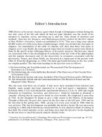
Figure 4.1 Schematic digram of the cardiovascular system following DeBoer [5]. Dashed lines in-
dicate slow sympathetic control, and solid lines indicate faster parasympathetic control.
The respiratory signal that drives the high-frequency variations in the model is
assumed to be unaffected by the other system parameters. DeBoer chose the respi-
ratory signal to be a simple sinusoid, although other investigations have explored
the use of more realistic signals [20]. DeBoer’s model was the first to allow for the
discrete (beat-to-beat) nature of the heart, whereas all previous models had used
continuous differential equations to describe the cardiovascular system. The model
consists of a set of difference equations involving systolic blood pressure (S), dias-
tolic pressure (D), pulse pressure (P = S −D), peripheral resistance (R), RR interval
(I), and an arterial time constant (T = RC), with C as the arterial compliance. The
equations are then based upon four distinct mechanisms:
1. Control of the HR and peripheral resistance by the baroreflex: The current
RR interval value, is a linear weighted combination of the last seven systolic
BP values (a
0
S
n
a
6
S
n−6
). The current systolic value, S
n
, represents the vagal
effect weighted by coefficient a
0
(fast with short delays), whereas S

n−2
S
n−6
represent sympathetic contributions (slower with longer delays). The previ-
ous systolic value, S
n−1
, does not contribute (a
1
= 0) because its vagal effect
has already died out and the sympathetic effect is not yet active.
2. Windkessel properties of the systemic arterial tree: This represents the sym-
pathetic action of the baroreflex on the peripheral resistance. The Windkessel
equation, D
n
= c
3
S
n−1
exp(−I
n−1
/T
n−1
), describes the diastolic pressure
P1: Shashi
August 24, 2006 11:42 Chan-Horizon Azuaje˙Book
106 Models for ECG and RR Interval Processes
decay, governed by the ratio of the previous RR interval to the previous
arterial time constant. The time constant of the decay, T
n
, and thus (assum-

ing a constant arterial compliance C) the current value of the peripheral
resistance, R
n
, depends on a weighted sum of the previous six values of S.
3. Contractile properties of the myocardium: The influence of the length of the
previous interval on the strength of the ventricular contraction is given by
P
n
= γ I
n−1
+c
2
, where γ and c
2
are physiological constants. A longer pulse
interval (I
n−1
> I
n−2
) therefore tends to increase the next pulse pressure
(if γ>0), P
n
, a phenomenon motivated by the increased filling of the ven-
tricles after a long interval, leading to a more forceful contraction (Starling’s
law) and by the restitution properties of the myocardium (which also leads
to an increased strength of contraction after a longer interval).
4. Mechanical effects of respiration on BP: Respiration is simulated by disturb-
ing P
n
with a sinusoidal variation in I. Without this addition, the equations

themselves do not imply any fluctuations in BP or HR but lead to stable
values for the different variables.
Linearization of the equations of motion around operating points (normal hu-
man values for S, D, I, and T) was employed to facilitate an analysis of the model.
Note that such a linearization is a good approximation when the subject is at rest.
The addition of a simulated respiratory signal was shown to provide a good cor-
respondence between the power spectra of real and simulated data. DeBoer also
pointed out the need to perform cross-spectral analysis between the RR tachogram,
the systolic BP, and respiration signals. Pitzalis et al. [21] performed such an analy-
sis supporting DeBoer’s model and showed that the respiratory rate modulates the
interrelationship between the RR interval and S variabilities: the higher the rate of
respiration, the smaller the gain and the smaller the phase difference between the
two. Furthermore, the same response is found after administering a β-adrenoceptor
blockade, suggesting that the sympathetic drive is not involved in this process.
Sleight and Casadei [7] also present evidence to support the assumptions underly-
ing the DeBoer model.
4.2.3 The Research Cardiovascular Simulator
The Research CardioVascular SIMulator (RCVSIM) [22–24] software
3
was devel-
oped in order to complement the experimental data sets provided by PhysioBank.
The human cardiovascular model underlying RCVSIM is based upon an electrical
circuit analog, with charge representing blood volume (Q, ml), current representing
blood flow rate ( ˙q, ml/s), voltage representing pressure (P, mmHg), capacitance rep-
resenting arterial/vascular compliance (C), and resistance (R) representing frictional
resistance to viscous blood flow. RCVSIM includes three major components.
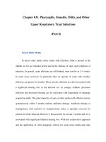
The first component (illustrated in Figure 4.2) is a lumped parameter model
of the pulsatile heart and circulation which itself consists of six compartments,
the left ventricles, the right ventricles, the systemic arteries, the systemic veins, the
3.

Open-source code and further details are available from />P1: Shashi
August 24, 2006 16:0 Chan-Horizon Azuaje˙Book
4.2 RR Interval Models 107
Figure 4.2 PhysioNet’s RCVSIM lumped parameter model of the human heart-lung unit in terms
of its electrical circuit analog. Charge is analogous to blood volume (Q, ml), current, to blood flow
rate (˙q, ml/s), and voltage, to pressure (P , mmHg). The model consists of six compartments which
represent the left and right ventricles (l,r ), systemic arteries and veins (a, v), and pulmonary arteries
and veins (pa, pv). Each compartment consists of a conduit for viscous blood flow with resistance
(R), a volume storage element with compliance (C ) and unstressed volume (Q
0
). The node labeled
P
”ra”
(t) is the location of where the right atrium would be if it were explicitly included in the model.
(Adapted from: [22] with permission.
c
 2006 R. Mukkamala.)
pulmonary arteries, and the pulmonary veins. Each compartment consists of a con-
duit for viscous blood flow with resistance (R), a volume storage element with
compliance (C) and unstressed volume (Q
0
). The second major component of the
model is a short-term regulatory system based upon the DeBoer model and includes
an arterial baroreflex system, a cardiopulmonary baroreflex system, and a direct
neural coupling mechanism between respiration and heart rate. The third major
component of RCVSIM is a model of resting physiologic perturbations which in-
cludes respiration, autoregulation of local vascular beds (exogenous disturbance to
systemic arterial resistance), and higher brain center activity affecting the autonomic
nervous system (1/ f exogenous disturbance to heart rate [25]).
The model is capable of generating realistically human pulsatile hemodynamic

waveforms, cardiac function and venous return curves, and beat-to-beat hemody-
namic variability. RCVSIM has been previously employed in cardiovascularresearch
P1: Shashi
August 24, 2006 11:42 Chan-Horizon Azuaje˙Book
108 Models for ECG and RR Interval Processes
by its author for the development and evaluation of system identification methods
aimed at the dynamical characterization of autonomic regulatory mechanisms [23].
Recent developments of RCVSIM have involved the development of a parallelized
version and extensions for adaptation to space-flight data to describe the processes
involved in orthostatic hypotension [26–28]. Simulink versions have been developed
both with and without the baroreflex reflex mechanism, and an additional intersti-
tial compartment to aid work fitting the model parameters to real data representing
an instance of hemorrhagic shock [29]. These recent innovations are currently be-
ing redeveloped into a platform-independent version which will shortly be available
from PhysioNet [22, 30].
4.2.4 Integral Pulse Frequency Modulation Model
The integral pulse frequency modulation (IPFM) model was developed for investi-
gating the generation of a discrete series of events, such as a series of heartbeats [31].
This model assumes the existence of a continuous-time input modulation signal
which possesses a particular physiological interpretation, such as describing the
mechanisms underlying the autonomic nervous system [32]. The action of this mod-
ulation signal when integrated through the model generates a series of interbeat
time intervals, which may be compared to RR intervals recorded from human
subjects.
The IPFM model assumes that the autonomic activity, including both the sym-
pathetic and parasympathetic influences, may be represented by a single modulating
input signal x(t). This input signal x(t) is integrated until a threshold, R, is reached
where a beat is generated. At this point, the integrator is reset to zero and the process
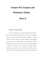
is repeated [31, 33] (see Figure 4.3). The beat-to-beat time series may be expressed
as a series of pulses,

p(t) = n =

t
n
0
1 + x(t)
T
dt, (4.3)
where n is an integer number representing the nth beat and t
n
reflects its time stamp.
The time T is the mean interbeat interval and x(t)/ T is the zero-mean modulating
term. It is usual to assume that this modulation term is relatively small (x(t) << 1)
Figure 4.3 The integral pulse frequency modulation model. The input signal x(t) is integrated
yielding y(t). When y(t) reaches the fixed reference value R, a pulse is emitted and the integrator
is reset to 0, whereupon the cycle starts again. Output of the model is the series of pulses p(t).
When used to model the cardiac pacemaker, the input is a signal proportional to the accelerating
autonomic efferences on the pacemaker cells and the output is the RR interval time series.
P1: Shashi
August 24, 2006 11:42 Chan-Horizon Azuaje˙Book
4.2 RR Interval Models 109
in order to reflect that heart rate variability is usually smaller than the mean heart
rate. The time-dependent value of (1 +x(t))/T may be viewed as the instantaneous
heart rate. For simplification, the first beat is assumed to occur at time t
0
= 0.
Generally, x(t) is assumed to be band-limited with negligible power for frequencies
greater than 0.4 Hz.
In physiological terms, the output signal of the integrator can be viewed as
the charging of the membrane potential of a sino-atrial pacemaker cell [34]. The

potential increases until a certain threshold (R in Figure 4.3) is exceeded and then
triggers an action potential which, when combined with the effect of many other
action potentials, initiates another cardiac cycle.
Given that the assumptions underlying the IPFM are valid, the aim is to con-
struct a method for obtaining information about the input signal x(t) using the
observed sequence of event times t
n
. The various issues concerning a reasonable
choice of time domain signal for representing the activity in the heart are discussed
in [32].
The IPFM model has been extended to provide a time-varying threshold inte-
gral pulse frequency modulation (TVTIPFM) model [35]. This approach has been
applied to RR intervals in order to discriminate between autonomic nervous mod-
ulation and the mechanical stretch induced effect caused by changes in the venous
return and respiratory modulation.
4.2.5 Nonlinear Deterministic Models
A chaotic dynamic system may be capable of generating a wide range of irregular
time series that would normally be associated with stochastic dynamics. The task of
identifying whether a particular set of observations may have arisen from a chaotic
system has given rise to a large body of research (see [36] and references therein). The
method of surrogate data is particularly useful for constructing hypothesis tests for
asking whether or not a given data set may have underlying nonlinear dynamics [37].
Nonlinear deterministic models come in a variety of forms ranging from local linear
models [38–40] to radial basis functions and neural networks [41, 42].
The first step when constructing a model using nonlinear time series analysis
techniques is to identify a suitable state space reconstruction. For a time series
s
n
,(n = 1, 2, , N), a delay coordinate reconstruction is obtained using
x

n
=

s
n−(m−1)τ
, , s
n−2τ
, s
n

(4.4)
where m and τ are known as the reconstruction dimension and delay, respectively.
The ability to accurately evaluate a particular reconstruction and compare various
models requires an incorporation of the measurement uncertainty inherent in the
data. McSharry and Smith give examples of how these techniques may be employed
when analysing three different experimental datasets [43]. In particular, this inves-
tigation presents a consistency check that may be used to identify why and where a
particular model is inadequate and suggests a means of resolving these problems.
Cao and Mees [44] developed a deterministic local linear model for analyzing
nonlinear interactions between heart rate, respiration, and the oxygen saturation
(SaO
2
) wave in the cardiovascular system. This model was constructed using
P1: Shashi
August 24, 2006 11:42 Chan-Horizon Azuaje˙Book
110 Models for ECG and RR Interval Processes
multichannel physiological signals from dataset B of the Santa Fe Time Series Com-
petition [45]. They found that it was possible to construct a model that provides
accurate forecasts of the next time step (next beat) in one signal using a combina-
tion of previous values selected from the other two signals. This demonstrates that

heart rate, respiration, and oxygen saturation are three key interacting factors in
the cardiorespiratory cycle since no other signal is required to provide accurate pre-
dictions. The investigation was repeated and it found similar results for different
segments of the three signals. It should be emphasized, however, that this analy-
sis was performed on only one subject who suffered from sleep apnea. In this
case, a strong correlation between respiration and the cardiovascular effort is to
be expected. For this reason, these results cannot be assumed to hold for normal
subjects and the results may indeed be specific to only the Santa Fe Time Series.
The question of whether parameters derived in specific situations are sufficiently
distinct such that they can be used to identify improving or worsening conditions
remains unanswered. A more detailed description of nonlinear techniques and their
application to filtering ECG signals can be found in Chapter 6.
4.2.6 Coupled Oscillators and Phase Synchronization
Observations of the phase differences between oscillations in HR, BP, and respira-
tion have shown that, although the phases drift in a highly nonstationary manner, at
certain times, phase locking can occur [3, 46, 47]. These observations led Rosen-
blum et al. [48–51] to propose the idea of representing the cardiovascular system
as a set of coupled oscillators, demonstrating that phase and frequency locking are
not equivalent. In the presence of noise, the relative phase performs a biased ran-
dom walk, resulting in no frequency locking, while retaining the presence of phase
locking.
Bra
ˇ
ci
ˇ
c et al. [47, 52, 53] then extended this model, consisting of five linearly
coupled oscillators,
˙x
i
=−x

i
q
i
− ω
i
y
i
+ g
x
i
(x)
˙y
i
=−y
i
q
i
+ ω
i
x
i
+ g
y
i
(y), q
i
= α
i



x
2
i
+ y
2
i
− a
i

(4.5)
where x, y are state vectors, g
x
i
(x) and g
y
i
(y) are linear coupling vectors, and α
i
,
a
i
, ω
i
are constants governing the individual oscillators. For each oscillator i, the
dynamics are described by the blood flow, x
i
, and the blood flow rate, y
i
.
Numerical simulation of this model generated signals which appeared similar

to the observed signals recorded from human subjects. This model with linear cou-
plings and added noise is capable of displaying similar forms of synchronization
as that observed for real signals. In particular, short episodes of synchronization
appear and disappear at random intervals as has been observed for human subjects.
One condition in which cardiorespiratory coupling is frequently observed is a
type of sleep known as noncyclic alternating phase (NCAP) sleep (see Chapter 3).
In fact, the changes in cardiovascular parameters over the sleep cycle and between
wakefullness and sleep are an active current research field which is only just being
explored (see [54–62]). In particular, Peng et al. [25, 57] have shown that the RR
P1: Shashi
August 24, 2006 11:42 Chan-Horizon Azuaje˙Book
4.2 RR Interval Models 111
interval exhibits some interesting long-range (circadian) scaling characteristics over
the 24-hour period (see Section 4.2.7). Since heart rate and HRV are known to be
correlated with activity and sleep [56], Lo et al. [62] later followed up this work to
show that the distribution of durations of wakefullness and sleep followed different
distributions; sleep episode durations follow a scale-free power law independent of
species, and sleep episode durations follow an exponential law with a characteristic
time scale related to body mass and metabolic rate.
4.2.7 Scale Invariance
Many complex biological systems display scale-invariant properties and the absence
of a characteristic scale (time and/or spatial domains) may suggest certain advan-
tages in terms of the ability to easily adapt to changes caused by external sources.
The traditional analysis of heart rate variability focuses on short time oscillations
related to respiration (approximately between 0.15 and 0.4 Hz) and the influence of
BP control mechanisms at approximately 0.1 Hz. The resting heartbeat of a healthy
human tends to vary in an erratic manner and casts doubt on the homeostatic view-
point of cardiovascular regulation in healthy humans. In fact, the analysis of a long
time series of heartbeat interval time series (typically over 24 hours) gives rise to
a1/ f -like spectrum for frequencies less than 0.1 Hz, suggesting the possibility of

scale-invariance in HRV [63].
The analysis of longrecords of RR intervals, with 24 hours giving approximately
10
5
data points, is possible using ambulatory (Holter) monitors. Peng et al. [25]
found that in the case of healthy subjects, these RR intervals display scale-invariant,
long-range anticorrelations up to 10
4
heartbeats. The histogram of increments of the
RR intervals may be described by a L
´
evy stable distribution.
4
Furthermore, a group
of subjects with severe heart disease had similar distributions but the long-range
correlations vanished. This suggests that the different scaling behavior in health
and disease must be related to the underlying dynamics of the cardiovascular
system.
A log-log plot of the power spectra, S( f ), of the RR intervals displays a linear
relationship, such that S( f ) ∼ f
β
. The value ofβ can be used to distinguish between:
(1) β = 0, an uncorrelated time series also known as “white noise”; (2) −1 <β<0,
correlated such that positive values are likely to be close in time to each other and
the same is true for negative values; and (3) 0 <β<1, anticorrelated time series
such that positive and negative values are more likely to alternate in time. The 1/f
noise, β = 1, often called “pink noise,” typically displayed by cardiac interbeat
intervals is an intermediate compromise between the randomness of white noise,
β = 0, and the much smoother Brownian motion, β = 2.
Although RR intervals from healthy subjects follow approximately β ∼ 1, RR

intervals from heart failure subjects have β ∼ 1.6, which is closer to Brownian
motion [65]. This variation in scaling suggests that the value of β may provide the
basis of a usefulmedical diagnostic. While there are a number of techniques available
4.
A heavy-tailed generalization of the normal distribution [64].
P1: Shashi
August 24, 2006 11:42 Chan-Horizon Azuaje˙Book
112 Models for ECG and RR Interval Processes
for quantifying self-similarity, detrended fluctuation analysis is often employed to
measure the self-similarity of nonstationary biomedical signals [66]. DFA provides
a scaling coefficient, α, which is related to β via β = 2α − 1.
McSharry and Malamud [67] compared five different techniques for quanti-
fying self-similarity in time series; these included power-spectral, wavelet variance,
semivariograms, rescaled-range, and detrended fluctuation analysis. Each technique
was applied to both normal and log-normal synthetic fractional noises and motions
generated using a spectral method, where a normally distributed white noise was
appropriately filtered such that its power-spectral density, S, varied with frequency,
f , according to S ∼ f
−β
. The five techniques provide varying levels of accuracy
depending on β and the degree of nonnormality of the time series being considered.
For normally distributed time series, semivariograms provide accurate estimates
for 1.2 <β<2.5, rescaled range for 0.0 <β<0.8, DFA for −0.8 <β<2.2,
and power spectra and wavelets for all values of β. All techniques demonstrate
decreasing accuracy for log-normal fractional noises with increasing coefficient of
variance, particularly for antipersistent time series. Wavelet analysis offers the best
performance both in terms of providing accurate estimates for normally distributed
time series over the entire range −2 ≤ β ≤ 4 and having the least decrease in
accuracy for log-normal noises.
The existence of a power law spectrum provides a necessary condition for scale

invariance in the process underlying heart rate variability. Ivanov et al. [68] demon-
strated that the normal healthy human heartbeat, even under resting conditions,
fluctuates in a complex manner and has a multifractal
5
temporal structure. Fur-
thermore, there was evidence of a loss of multifractality (to monofractality) in cases
of congestive heart failure. Scaling techniques adapted from statistical physics have
revealed the presence of long-range, power-law correlations, as part of multifractal
cascades operating over a wide range of time scales (see [65, 68] and references
therein).
A number of different statistical models have been proposed to explain the
mechanisms underlying the heart rate variability of healthy human subjects. Lin
and Hughson [69] present a model motivated by an analogy with turbulence. This
approach provides a cascade-type multifractal model for determining the defor-
mation of the distribution of RR intervals. One feature of such a model is that
of evolving from a Gaussian distribution at small scales to a stretched exponen-
tial at smaller scales. Kiyono et al. [70] argue that the healthy human heart rate
is controlled to converge continually to a critical state and show that their model
is capable of providing a better fit to the observed data than that of the random
(multiplicative) cascade model reported in [69]. Kuusela et al. [71] present a model
based on a simple one-dimensional Langevin-type stochastic difference equation,
which can describe the fluctuations in the heart rate. This model is capable of ex-
plaining the multifractal behavior seen in real data and suggests how pathologic
cases simplify the heart rate control system.
5.
Monofractal signals are homogeneous in that only one scaling exponent is needed to describe all segments
of the signal. In contrast, multifractal signals requires a range of different exponents to explain their scaling
properties.
P1: Shashi
August 24, 2006 11:42 Chan-Horizon Azuaje˙Book

4.2 RR Interval Models 113
4.2.8 PhysioNet Challenge
The PhysioNet challenge of 2002
6
invited participants to design a numerical model
for generating 24-hour records of RR intervals. A second part of the challenge
asked participants to use their respective signal processing techniques to identify
the real and artificial records from among a database of unmarked 24-hour RR
tachograms. The wide range of models entered for the competition reflects the nu-
merous approaches available for investigating heart rate variability. The following
paragraphs summarize these approaches, which include a multiplicative cascade
model, a Markovian model, and a heuristic multiscale approach based on empirical
observations.
Lin and Hughson [69] explored the multifractal HRV displayed in healthy
and other physiological conditions, including autonomic blockades and congestive
heart failure, by using a multiplicative random cascade model. Their method used
a bounded cascade model to generate artificial time series which was able to mimic
some of the known phenomenology of HRV in healthy humans: (1) multifractal
spectrum including 1/ f power law, (2) the transition from stretch-exponential to
Gaussian probability density function in the interbeat interval increment data and
(3) the Poisson excursion law in small RR increments [72]. The cascade consisted
of a discrete fragmentation process and assigned random weights to the cascade
components of the fragmented time intervals. The artificial time series was finally
constructed by multiplying the cascade components in each level.
Yang et al. [73] employed symbolic dynamics and probabilistic automaton to
construct a Markovian model for characterizing the complex dynamics of healthy
human heart rate signals. Their approach was to simplify the dynamics by mapping
the output to binary sequences, where the increase and decrease of the interbeat
interval were denoted by 1 and 0, respectively. In this way, it was also possible to
define a m-bit symbolic sequence to characterize transitions of symbolic dynamics.

For the simplest model consisting of 2-bit sequences, there are four possible sym-
bolic sequences including 11, 10, 00, and 01. Moreover, each symbolic sequence
has two possible transitions, for example, 1(0) can be transformed to (0)0, which
results in decreasing RR intervals, or (0)1 and vice versa. In order to define the
mechanism underlying these symbolic transitions, the authors utilized the concept
of probabilistic automaton in which the transition from current symbolic sequence
to next state takes place with a certain probability in a given range of RR intervals.
The model used 8-bit sequences and a probability table obtained from the RR time
series of healthy humans from Taipei Veterans General Hospital and PhysioNet.
The resulting generator is comprised of the following major components: (1) the
symbolic sequence as a state of RR dynamics, (2) the probability table defining
transitions between two sequences, and (3) an absolute Gaussian noise process for
governing increments of RR intervals.
McSharry et al. [74] used a heuristic empirical approach for modeling the
fluctuations of the beat-to-beat RR intervals of a normal healthy human over
24 hours by considering the different time scales independently. Short range vari-
ability due to Mayer waves and RSA were incorporated into the algorithm using a
6.
See for more details.
P1: Shashi
August 24, 2006 11:42 Chan-Horizon Azuaje˙Book
114 Models for ECG and RR Interval Processes
power spectrum with given spectral characteristics described by its low frequency
and high frequency components, respectively [75]. Longer range fluctuations aris-
ing from transitions between physiological states were generated using switching
distributions extracted from real data. The model generated realistic synthetic 24-
hour RR tachograms by including both cardiovascular interactions and transitions
between physiological states. The algorithm included the effects of various physi-
ological states, including sleep states, using RR intervals with specific means and
trends. An analysis of ectopic beat and artifact incidence in an accompanying pa-

per [76] was usedto provide a mechanism for generating realistic ectopy and artifact.
Ectopic beats were added with an independent probability of one per hour. Artifacts
were included with a probability proportional to mean heart rate within a state and
increased for state transition periods. The algorithm provides RR tachograms that
are similar to those in the MIT-BIH Normal Sinus Rhythm Database.
4.2.9 RR Interval Models for Abnormal Rhythms
Chapter 1 described some of the mechanisms that activate and mediate arrhythmias
of the heart. Broadly speaking, modeling of arrhythmias can be broken down into
two subgroups: ventricular arrhythmias and atrial arrhythmias. The models tend
to describe either the underlying RR interval processes or the manifest waveform
(ECG). Furthermore, the models are formulated either from the cellular conduction
perspective (usually for RR interval models) or from an empirical standpoint. Since
the connection between the underlying beat-to-beat interval process and the resul-
tant waveform is complex, empirical models of the ECG waveform are common.
These include simple time domain templates [77], Fourier and AR models [78],
singular value decomposition-based techniques [79, 80], and more complex meth-
ods such as neural network classifiers [81–83], and finite element models [84]. Such
models are usually applied on a beat-by-beat basis. Furthermore, due to the fact that
the classifiers are trained using a cost function based upon a distance metric between
waveforms, small deviations in the waveform morphology (such as that seen in atrial
arrhythmias) are often poorly identified. In the case of atrial arrhythmias, unless
a full three-dimensional model of the cardiac potentials is used (such as in Cherry
et al. [85]), it is often more appropriate to analyze the RR interval process itself.
The following gives a chronological summary of the developments in modeling
atrial fibrillation. In 1983, Cohen et al. [86] introduced a model for the ventricular
response during AF that treated the atrio-ventricular junction as a lumped parameter
structure with defined electrical properties such as the refactory period and period
of autorhymicity, that is being continually bombarded by random AF impulses.
Although this model could account for all the principal statistical properties of the
RR interval distribution during AF, several important physiological properties of

the heart were not included in the model (such as conduction delays within the AV
junction and ventricle and the effect of ventricular pacing).
In 1988, Wittkampf et al. [87–89] explained the fact that short RR intervals
during AF could be eliminated by ventricular pacing at relatively long cycle lengths
through a model that modulates the AV node pacemaker rate and rhythm by AF
impulses. However, this model failed to explain the relationship between most of
the captured beats and the shortest RR interval length in a canine model.
P1: Shashi
August 24, 2006 11:42 Chan-Horizon Azuaje˙Book
4.3 ECG Models 115
In 1996, Meijler et al. [90] proposed an alternative model whereby the irreg-
ularity of RR intervals during AF are explained by modulation of the AV node
through concealed AF impulses resulting in an inverse relationship between the
atrial and ventricular rates. Unfortunately, recent clinical results do not support this
prediction.
Around the same time Zeng and Glass [91] introduced an alternative model
of AV node conduction which was able to correctly model much of the statistical
distribution of the RR intervals during AF. This model was later extended by Tateno
and Glass [92] and Jorgensen et al. [93] and includes a description of the AV delay
time, τ
AV D
, (which is known to be dependent on the AV junction recovery time)
given by
τ
AV D
= τ
AV D
mi n
+ αe
−T

R
/c
(4.6)
where T
R
is the AV junction recovery time, τ
AV D
mi n
is the minimum AV delay when
T
R
→∞, α is the maximum extension of the AV delay when T
R
= 0, and c is a time
constant. Although this extension modeled many of the properties of AF, it failed
to account for the dependence of the refactory period, τ
R
, on the heart rate (the
higher the heart rate, the shorter the refactory period) [86].
Lian et al. [94] recently proposed an extension of Cohen’s model [86] which
does model the refactory behavior of the AV junction as
τ
AV J
= τ
AV J
mi n
+ τ
AV J
ext
(1 −e

−T
R
/τ
ext
) (4.7)
where τ
AV J
mi n
is the shortest AV junction refactory period corresponding to T
R
= 0
and τ
AV J
ext
is the maximum extension of the refactory period when T
R
→∞. The AV
delay (4.6) is also included in this model together with a function which expresses the
modulation of the AV junction refactory period by blocked impulses. If an impulse
is blocked by the refactory AV junction, τ
AV J
is prolonged by the concealed impulse
such that
τ
AV J
→ τ
AV J
+ τ
AV J
mi n


t
τ
AV J

θ

max

1,
V
(V
T
− V
R
)

δ
(4.8)
where V/(V
T
−V
R
) is the relative amplitude of the AF pulses and t (0 < t <τ
AV J
)
is the time when the impulse is blocked. θ and δ are independent parameters which
modulate the timing and duration of the blocked impulse. With suitably chosen
values for the above parameters, this model can account for all the statistical prop-
erties of observed RR intervals processes during AF (see Lian et al. [94] for further

details and experimental results).
4.3 ECG Models
The following sections show two disparate approaches to modeling the ECG. While
both paradigms can produce an ECG signal and are consistent with various as-
pects of the physiology, they attempt to replicate different observed phenomena on
P1: Shashi
August 24, 2006 11:42 Chan-Horizon Azuaje˙Book
116 Models for ECG and RR Interval Processes
different temporal scales. Section 4.3.1 presents the first approach, based on com-
putational physiology, which employs first principles to derive the fundamental
equations and then integrates this information using a three-dimensional anatomi-
cal description of the heart. This approach, although complex and computationally
intensive, often provides a model which furthers our understanding of the effects of
small changes or defects in cardiac physiology. Section 4.3.2 describes the second
approach which appeals to an empirical description of the ECG, whereby statistical
quantities such as the temporal and spectral characteristics of both the ECG and
associated heart rate are modeled. Given that these quantities are routinely used for
clinical diagnosis, this latter approach is of interest in the field of biomedical signal
processing.
4.3.1 Computational Physiology
While the ECG is routinely used to diagnose arrhythmias, it reflects an integrated
signal and cannot provide information on the micro-spatial scales of cells and ionic
channels. For this reason, the field of computational cardiac modeling and simu-
lation has grown over the last decade. In the following, we consider a variety of
approaches to whole heart modeling.
The fundamental approach to whole heart modeling is based on the finite ele-
ment method, which partitions the entire heart and chest into numerous elements
where each element represents a group of cells. The ECG may then be simulated by
calculating the body surface potential of each cardiac element [95]. This approach,
however, fails to relate the ECG waveform with the micro-scale cellular electrophys-

iology. The use of membrane equations is needed to incorporate the mechanisms at
cell, channel, and molecular level [96]. In the following, we review some promis-
ing research in the area of whole heart modeling, such as cellular autonoma and
multiscale modeling approaches.
Arrhythmias are often initiated by abnormal electrical activity at the cellular
scale or the ionic channel level. Cellular automata provide an effective means of
constructing whole heart models and of simulating such arrhythmias, which may
display a spatio-temporal evolution within the heart [97]. Such models combine a
differential description of electrical properties of cardiac cells using membrane equa-
tions. This approach relates the ECG waveform to the underlying cellular activity
and is capable of describing a range of pathological conditions. Cluster computing
is employed as a means of dealing with the necessary computationally intensive
simulations.
A single autonoma cell may be viewed as a computing unit for the action po-
tential and ECG simulation. The electrical activity of these cells is described by
corresponding Hodgkin-Huxley action potential equations. Zhu et al. [97] con-
structed a three-dimensional heart model based on data from the axial images of
the Visible Human Project digital male cadaver [98]. The anatomical model of the
heart utilized a data file to describe the distribution of the cell array and the char-
acteristics of each cell.
Understanding the complexity of the heart requires biological models of cells,
tissues, organs, and organ systems. The present aim is to combine the bottom-
up approach of investigating interactions at the lower spatial scales of proteins
P1: Shashi
August 24, 2006 11:42 Chan-Horizon Azuaje˙Book
4.3 ECG Models 117
(receptors, transporters, enzymes, and so forth) with that of the top-down approach
of modeling organs and organ systems [99]. Such a multiscale integrative approach
relies on the computational solution of physical conservation laws and anatomically
detailed geometric models [100].

Multiscale models are now possible because of three recent developments:
(1) molecular and biophysical data on many proteins and genes is now available
(e.g., ion transporters [101]); (2) models exist which can describe the complexity of
biological processes [99]; and (3) continuing improvements in computing resources
allow the simulation of complex cell models with hundreds of different protein
functions on a single-processor computer whereas parallel computers can now deal
with whole organ models [102].
The interplay between simulation and experimentation has given rise to models
of sufficient accuracy for use in drug development. Numerous drugs have to be
withdrawn during trials due to cardiac side effects that are usually associated with
irregular heartbeats and abnormal ECG morphologies. Noble and Rudy [103] have
constructed a model of the heart that is able to provide an accurate description at
the cellular level. Simulations of this model have been of great value to improving
the understanding of the complex interactions underlying the heart. Furthermore,
such computer-based heart models, known as in silico screening, provide a means
of simulating and understanding the effects of drugs on the cardiovascular system.
In particular these models can now be used to investigate the regulation of drug
therapy.
While the grand challenge of heart modeling is to simulate a full-scale coronary
heart attack, this would require extensive computing power [99]. Another hindrance
is the lack of transfer of both data and models between different research centers.
In addition, there is no standard representation for these models, thereby limiting
the communication of innovative ideas and decreasing the pace of research. Once
these hurdles have been overcome, the eventual aim is the development of integrated
models comprising cells, organs, and organ systems.
4.3.2 Synthetic Electrocardiogram Signals
When only a realistic ECG is required (such as in the testing of signal processing
algorithms), we may use an alternative approach to modeling the heart. ECGSYN
is a dynamical model for generating synthetic ECG signals with arbitrary mor-
phologies (i.e., any lead configuration) where the user has the flexibility to choose

the operating characteristics. The model was motivated by the need to evaluate
and quantify the performance of the signal processing techniques on ECG signals
with known characteristics. An early attempt to produce a synthetic ECG gener-
ator [104] (available from the PhysioNet Web site [30] along with ECGSYN) is
not intended to be highly realistic, and includes no P wave, and no variations in
timing or morphology and discontinuities. In contrast to this, ECGSYN is based
upon time-varying differential equations and is continuous with convincing beat-
to-beat variations in morphology and interbeat timing. ECGSYN may be employed
to generate extremely realistic ECG signals with complete flexibility over the choice
of parameters that govern the structure of these ECG signals in both the temporal
and spectral domains. The model also allows the average morphology of the ECG
P1: Shashi
August 24, 2006 11:42 Chan-Horizon Azuaje˙Book
118 Models for ECG and RR Interval Processes
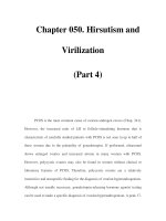
Figure 4.4 ECGSYN flow chart describing the procedure for specifying the temporal and spectral
description of the RR tachogram and ECG morphology.
to be fully specified. In this way, it is possible to simulate ECG signals that show
signs of various pathological conditions.
Open-source code in Matlab and C and further details of the model may be
obtained from the PhysioNet Web site.
7
In addition a Java applet may be utilised
in order to select model parameters from a graphical user interface, allowing the
user to simulate and download an ECG signal with known characteristics. The
underlying algorithm consists of two parts. The first stage involves the generation of
an internal time series with internal sampling frequency f
int
to incorporate a specific
mean heart rate, standard deviation and spectral characteristics corresponding to
a real RR tachogram. The second stage produces the average morphology of the

ECG by specifying the locations and heights of the peaks that occur during each
heartbeat. A flow chart of the various processes in ECGSYN for simulating the
ECG is shown in Figure 4.4.
Spectral characteristics of the RR tachogram, including both RSA and Mayer
waves, are replicated by describing a bimodal spectrum composed of the sum of
7.
See />P1: Shashi
August 24, 2006 11:42 Chan-Horizon Azuaje˙Book
4.3 ECG Models 119
Figure 4.5 Spectral characteristics of (4.9), the RR interval generator for ECGSYN.
two Gaussian functions,
S( f ) =
σ
2
1

2πc
2
1
exp

( f − f
1
)
2
2c
2
1

+

σ
2
2

2πc
2
2
exp

( f − f
2
)
2
2c
2
2

(4.9)
with means f
1
, f
2
and standard deviations c
1
, c
2
. Power in the LF and HF bands is
given by σ
2
1

and σ
2
2
, respectively, whereas the variance equals the total area σ
2
=
σ
2
1
+ σ
2
2
and the LF/HF ratio is σ
2
1
/σ
2
2
(see Figure 4.5).
A time series T(t) with power spectrum S( f ) is generated by taking the inverse
Fourier transform of a sequence of complex numbers with amplitudes
√
S( f ) and
phases that are randomly distributed between 0 and 2π . By multiplying this time
series by an appropriate scaling constant and adding an offset value, the resulting
time series can be given any required mean and standard deviation. Different real-
izations of the random phases may be specified by varying the seed of the random
number generator. In this way, many different time series T(t) may be generated
with the same temporal and spectral properties. Alternatively a real RR interval
time series could be used instead. This has the advantage of increased realism, but

the disadvantage of unknown spectral properties of the RR tachogram. However,
if all the beat intervals are from sinus beats, the Lomb periodogram can produce
an accurate estimate of the spectral characteristics of the time series [105, 106].
During each heartbeat, the ECG traces a quasi-periodic waveform where the
morphology of each cycle is labeled by its peaks and troughs, P, Q, R, S, and T, as
shown in Figure 4.6. This quasi-periodicity can be reproduced by constructing a
dynamical model containing an attracting limit cycle; each heartbeat corresponds
to one revolution around this limit cycle, which lies in the (x, y)-plane as shown in
Figure 4.7. The morphology of the ECG is specified by using a series of exponentials
P1: Shashi
August 24, 2006 11:42 Chan-Horizon Azuaje˙Book
120 Models for ECG and RR Interval Processes
Figure 4.6 Two seconds of synthetic ECG reflecting the electrical activity in the heart during two
beats. Morphology is shown by five extrema P, Q, R, S, and T. Time intervals corresponding to the
RR interval and the surrogate QT interval are also indicated.
Figure 4.7 Three-dimensional state space of the dynamical system given by integrating (4.10)
showing motion around the limit cycle in the horizontal (x, y)-plane. The vertical z-component pro-
vides the synthetic ECG signal with a morphology that is defined by the five extrema P, Q, R, S,
and T.
P1: Shashi
August 24, 2006 11:42 Chan-Horizon Azuaje˙Book
4.3 ECG Models 121
to force the trajectory to trace out the PQRST-waveform in the z-direction. A series
of five angles, (θ
P
, θ
Q
, θ
R
, θ

S
, θ
T
), describes the extrema of the peaks (P, Q, R, S, T),
respectively.
The dynamical equations of motion are given by three ordinary differential
equations [107],
˙x = αx − ωy
˙y = αy + ωx
˙z =−

i∈{P, Q, R, S,T
−
,T
+
}
a
i
θ
i
exp(−θ
2
i
/2b
2
i
) − (z − z
0
) (4.10)
where α = 1 −


x
2
+ y
2
, θ
i
= (θ − θ
i
) mod 2π, θ = atan2(y, x) and ω is the
angular velocity of the trajectory as it moves around the limit cycle. The coefficients
a
i
govern the magnitude of the peaks whereas the b
i
define the width (time duration)
of each peak. Note that the T wave is often asymmetrical and therefore requires
two Gaussians, T
−
and T
+
(rather than one), to correctly model this asymmetry
(see [108]). Baseline wander may be introduced by coupling the baseline value z
0
in (4.10) to the respiratory frequency f
2
in (4.9) using z
0
(t) = Asin(2π f
2

t). The
output synthetic ECG signal, s(t), is the vertical component of the three-dimensional
dynamical system in (4.10): s(t) = z(t).
Having calculated the internal RR tachogram expressed by the time series T(t)
with power spectrum S( f ) given by (4.9), this can then be used to drive the dy-
namical model (4.10) so that the resulting RR intervals will have the same power
spectrum as that given by S( f ). Starting from the auxiliary
8
time t
n
, with angle
θ = θ
R
, the time interval T(t
n
) is used to calculate an angular frequency 
n
=
2π
T(t
n
)
.
This particular angular frequency, 
n
, is used to specify the dynamics until the an-
gle θ reaches θ
R
again, whereby a complete revolution (one heartbeat) has taken
place. For the next revolution, the time is updated, t

n+1
= t
n
+ T(t
n
), and the next
angular frequency, 
n+1
=
2π
T(t
n+1
)
, is used to drive the trajectory around the limit
cycle. In this way, the internally generated beat-to-beat time series, T(t), can be
used to generate an ECG signal with associated RR intervals that have the same
spectral characteristics. The angular frequency ω(t) in (4.10) is specified using the
beat-to-beat values 
n
obtained from the internally generated RR tachogram:
ω(t) = 
n
, t
n
≤ t < t
n+1
(4.11)
A fourth-order Runge-Kutta method [109] is used to integrate the equations
of motion in (4.10) using the beat-to-beat values of the angular frequency . The
time series T(t) used for defining the values of 

n
has a high sampling frequency of
f
int
, which is effectively the step size of the integration. The final output ECG signal
is then downsampled to f
ecg
if f
int
> f
ecg
by a factor of
f
int
f
ecg
in order to generate
an ECG signal at the requested sampling frequency. In practice f
int
is taken as an
integer multiple of f
ecg
for simplicity.
8.
This auxiliary time axis is used to calculate the values of 
n
for consecutive RR intervals, whereas the time
axis for the ECG signal is sampled around the limit cycle in the (x, y)-plane.
P1: Shashi
August 24, 2006 11:42 Chan-Horizon Azuaje˙Book

122 Models for ECG and RR Interval Processes
Table 4.1 Morphological Parameters of the ECG Model with Modulation Factor α =

h
mean
/60
Index (i) P Q R S T
−
T
+
Time (seconds) −0.2
√
α −0.05α 0 0.05α 0.277
√
α 0.286
√
α
θ
i
(radians) −
π
√
α
3
−
πα
12
0
πα
12

5π
√
α
9
−
π
√
α
60
5π
√
α
9
a
i
0.8 −5.0 30.0 −7.50.5α
2.5
0.75α
2.5
b
i
0.2α 0.1α 0.1α 0.1α 0.4α
−1
0.2α
The size of the mean heart rate affects the shape of the ECG morphology. An
analysis of real ECG signals from healthy human subjects for different heart rates
shows that the intervals between the extrema vary by different amounts; in par-
ticular, the QRS width decreases with increasing heart rate. This is as one would
expect; when sympathetic tone increases, the conduction velocity across the ven-
tricles increases together with an augmented heart rate. The time for ventricular

depolarization (represented by the QRS complex of the ECG) is therefore shorter.
These changes are replicated by modifying the width of the exponentials in (4.10)
and also the positions of the angles θ. This is achieved by using a heart rate de-
pendent factor α =
√
h
mean
/60 where h
mean
is the mean heart rate expressed in
units of bpm (see Table 4.1). The well-documented [110] asymmetry of the T wave
and heart rate related changes in the T wave [111] are emulated by adding an ex-
tra Gaussian to the T wave section (denoted T
−
and T
+
because they are placed
just before and just after the peak of the T wave in the original model). To repli-
cate the increasing T wave symmetry and amplitude observed with increasing heart
rate [111], the Gaussian heights associated with the T wave are increased by an
empirically derived factor α
2.5
. The increasing symmetry for increasing heart rates
is emulated by shrinking a
T+
by a factor α
−1
. Perfect T wave symmetry would
therefore be achieved at about 134 bpm if a
T+

= a
T−
(0.4α
−1
= 0.2α). In practice,
this symmetry is asymptotic as a
T+
=a
T−
. In order to employ ECGSYN to simulate
an ECG signal, the user must select from the list of parameters given in Tables 4.1
and 4.2, which specify the model’s behavior in terms of its spectral characteristics
given by (4.9) and time domain dynamics given by (4.10).
As illustrated in Figure 4.8, ECGSYN is capable of generating realistic ECG
signals for a range of heart rates. The temporal modulating factors provided in
Table 4.2 Temporal and Spectral Parameters of the ECG Model
Description Notation Defaults
Approximate number of heartbeats N 256
ECG sampling frequency f
ecg
256 Hz
Internal sampling frequency f
int
512 Hz
Amplitude of additive uniform noise A 0.1 mV
Heart rate mean h
mean
60 bpm
Heart rate standard deviation h
std

1 bpm
Low frequency f
1
0.1 Hz
High frequency f
2
0.25 Hz
Low-frequency standard deviation c
1
0.1 Hz
High-frequency standard deviation c
2
0.1 Hz
LF/HF ratio γ 0.5
P1: Shashi
August 24, 2006 11:42 Chan-Horizon Azuaje˙Book
4.3 ECG Models 123
Figure 4.8 Synthetic ECG signals for different mean heart rates: (a) 30 bpm, (b) 60 bpm, and
(c) 120 bpm.
Table 4.1 ensure that the various intervals, such as the PR, QT, and QRS, decrease
with increasing heart rate. A nonlinear relationship between the morphology mod-
ulation factor α and the mean heart rate h
mean
decreases the temporal contraction of
the overall PQRST morphology with respect to the refractory period (the minimum
amount of time in which depolarization and repolarization of the cardiac muscle
can occur). This is consistent with the changes in parasympathetic stimulation con-
nected to changes in heart rate; a higher heart rate due to sympathetic stimulation
leads to an increase in conduction velocity across the ventricles and an associated
reduction in QRS width. Note that the changes in angular frequency, ω, around the

limit cycle, resulting from the period changes in each RR interval, do not lead to
temporal changes, but to amplitude changes. For example, decreases in RR interval
(higher heart rates) will not only lead to less broad QRS complexes, but also to
lower amplitude R peaks, since the limit cycle will have less time to reach the max-
imum value of the Gaussian contribution given by a
R
, b
R
, and θ
R
. This realistic
(parasympathetically mediated) amplitude variation [112, 113], which is due to
respiration-induced mechanical changes in the heart position with respect to the
electrode positions in real recordings, is dominated by the high-frequency com-
ponent in (4.9), which reflects parasympathetic activity in our model. This phe-
nomenon is independent of the respiratory-coupled baseline wander in this model
which is coupled to the peak HF frequency in a rather ad hoc manner. Of course,
this part of the model could be made more realistic by coupling the baseline wander
to a phase-lagged signal derived from highpass filtering (f
c
= 0.15 Hz) the RR
P1: Shashi
August 24, 2006 11:42 Chan-Horizon Azuaje˙Book
124 Models for ECG and RR Interval Processes
interval time series. The phase lag is important, since RSA and mechanical effects
on the ECG and RR time series are not in phase (and often drift based on a sub-
ject’s activity [3]). The beat-to-beat changes in RR intervals in this model faithfully
reproduce RSA effects (decreases in RR interval with inspiration and increases with
expiration) for lead configurations taken in the sense of lead I. Therefore, although
the morphologies in the figures are modeled after lead II or V5, the amplitude mod-

ulation of the R peaks acts in the opposite sense to that which is seen on real lead II
or V5 electrode configurations. That is, on inspiration (expiration) the amplitude
of the model-derived R peaks decrease (increase) rather than increase (decrease).
This is a reflection of the fact that these changes are a mechanical artifact on real
ECG recordings, rather than a direct result of the neural mediated mechanisms.
(A recent addition to the model, proposed by Amann et al. [114], includes an
amplitude modulation term in ˙z in (4.10) and may be used to provide the required
modulation in such cases.) Furthermore, the phase lag between the RSA effect and
the R peak modulation effect is fixed, reflecting the fact that this model is assum-
ing a stationary state for each instance of generation. Extensions to this model, to
couple it to a 24-hour RR time series, were presented in [115], where the entire
sequence was composed of a series of RR tachograms, each having a stationary
state with different characteristics reflecting observed normal circadian changes
(see [74] and Section 4.2.8).
ECGSYN can be employed to generate ECG signals with known spectral char-
acteristics and can be used to test the effect of varying the ECG sampling fre-
quency f
ecg
on the estimation of HRV metrics. In the following analysis, estimates
of the LF/HF ratio were calculated for a range of sampling frequencies (Figure 4.9).
ECGSYN was operated using a mean heart rate of 60 bpm, a standard deviation of
3 bpm, and a LF/HF ratio of 0.5. Error bars representing one standard deviation
on either side of the means (dots) using a total of 100 Monte Carlo runs are also
shown.
The LF/HF ratio was estimated using the Lomb periodogram. As this tech-
nique introduces negligible variance into the estimate [105, 106, 116], it may be
concluded that the underestimation of the LF/HF ratio is due to the sampling fre-
quency being too small. The analysis indicates that the LF/HF ratio is considerably
underestimated for sampling frequencies below 512 Hz. This result is consistent
with previous investigations performed on real ECG signals [61, 106, 117]. In ad-

dition, it provides a guide for clinicians when selecting the sampling frequency of
the ECG based on the required accuracy of the HRV metrics.
The key features of ECGSYN which make this type of model such a useful tool
for testing signal processing algorithms are as follows:
1. A user can rapidly generate many possible morphologies at a range of heart
rates and HRVs (determined separately by the standard deviation and the
LF/HF ratio). An algorithm can therefore be tested on a vast range of ECGs
(some of which can be extremely rare and therefore underrepresented in
databases).
2. The sampling frequency can be varied and the response of an algorithm can
be evaluated.
P1: Shashi
August 24, 2006 11:42 Chan-Horizon Azuaje˙Book
4.3 ECG Models 125
Figure 4.9 LF/HF ratio estimates computed from synthetic ECG signals for a range of sampling
frequencies using an input LF/HF ratio of 0.5 (horizontal line). The distribution of estimates is shown
by the mean (dot) and plus/minus one standard deviation error bars. The simulations used 100
realizations of noise-free synthetic ECG signals with a mean heart rate of 60 bpm and standard
deviation of 3 bpm.
3. The signal is noise free, so noise may be incrementally added and a filter re-
sponse at different frequencies and noise levels can be evaluated for differing
physiological events.
4. Abnormal events (such as arrhythmias or ST-elevation) may be incorporated
into the algorithm, and detectors of these events can be evaluated under
varying noise conditions and for a variety of morphologies.
Although the model is designed to provide a realistic emulation of a sinus rhythm
ECG, the fact that the RR interval process can be decoupled from the waveform
generator, it is possible to reproduce the waveforms of particular arrhythmias by
selecting a suitable RR interval process generator and altering the morphological
parameters (θ

i
, a
i
, and b
i
) together with the number of events, i, on the limit cycle.
Healey et al. [118] have used ECGSYN to simulate AF by extending the AF RR in-
terval model of Zeng and Glass [91] and coupling the conducted and nonconducted
RR intervals to two different ECGSYN models (one with no P wave and one with
only a P wave). Moreover, the concept behind ECGSYN could be used to sim-
ulate any quasi-periodic signal. In [119] the model was extended to produce BP
and respiration waveforms, with realistic coupling to the ECG. The model has
also been use to generate a 12-lead simulator for training in coronary artery dis-
ease identification as part of American Board of Family Practice Maintenance of
P1: Shashi
August 24, 2006 11:42 Chan-Horizon Azuaje˙Book
126 Models for ECG and RR Interval Processes
Figure 4.10 Example of a 12-lead version of ECGSYN, produced for [120] by Dr. Guy Roussel of
the American Board of Family Practice. Standard lead labels and graph paper has been used. One
small square = 1 mm, = 0.1 mV amplitude vertically (one large square = 0.5 mV) and 5 large
boxes horizontally represent 1 second; paper moves at 25 mm/s. (From: [120].
c
 2006 Guy Roussel.
Reproduced with permission.)
Certification [120]. An example of a 12-lead output from the model can be found
in Figure 4.10. The model has also been used to generate realistic ST-depressions
on leads V5 and V6.
Other recent developments have included the automatic derivation of model
parameters for a specific patient [108], and the transposition of the differential
equations into polar coordinates [114, 121]. Further developments to improve the

model should include the variation of ω within the limit cycle (to reflect changes
in conduction velocity) and the generalization to a three-dimensional dipole model.
These are current active areas of research (see [122]). Chapter 6 illustrates the appli-
cation of the ECG model to filtering, compression and parameter extraction through
a gradient descent, including a Kalman filter formulation to track the changes in
the model parameters over time.
4.4 Conclusion
The models presented in this chapter are intended to provide the reader with an
overview of the variety of cardiovascular models available to the researcher. Models
for describing RR interval dynamics and ECG signals range from physiological-
based to data-based approaches. The motivation behind these models often varies
with the intended application: whether to improve understanding of the underlying
P1: Shashi
August 24, 2006 11:42 Chan-Horizon Azuaje˙Book
4.4 Conclusion 127
control mechanisms or to attempt to obtain a better fit to the observed biomedical
signals.
Applications of these models have included model fitting [29, 108], compres-
sion and filtering [119, 123], and classification [124]. However, the required com-
plexity for realistic models (particularly for ECG generation) has limited the devel-
opment of using model parameters for classifying hemodynamic and cardiac states.
The assumed increase in computing power and utilization of parallel processing
is likely to stimulate research in these fields in the near future. Simplified (and
tractable) models such as ECGSYN provide a realistic current alternative. Chapter
6 describes a model fitting procedure that can run on a beat-by-beat basis in real
time on a modern desktop computer.
Computational physiology is now at the stage where it is possible to integrate
models from the level of the cell to that of the organ. By taking a multidisciplinary
approach to systems biology, the ability to construct in silico models that reflect the
underlying physiology and match the observed signals has the potential to deliver

considerable advances in the field of biomedical science.
References
[1] Hales, S., Statical Essays II, Haemastaticks, London, U.K.: Innings and Manby, 1733.
[2] Ludwig, C., “Beitr
¨
age zur Kenntnis des Einflusses der Respirationsbewegung auf den
Blutlauf im Aortensystem,” Arch. Anat. Physiol., Vol. 13, 1847, pp. 242–302.
[3] Hoyer, D., et al., “Validating Phase Relations Between Cardiac and Breathing Cycles
During Sleep,” IEEE Eng. Med. Biol., March/April 2001.
[4] Thomas, R. J., et al., “An Electrocardiogram-Based Technique to Assess Cardiopul-
monary Coupling During Sleep,” Sleep, Vol. 28, No. 9, October 2005, pp. 1151–
1161.
[5] DeBoer, R. W., J. M. Karemaker, and J. Strackee, “Hemodynamic Fluctuations and
Baroreflex Sensitivity in Humans: A Beat-to-Beat Model,” Am. J. Physiol., Vol. 253,
1987, pp. 680–689.
[6] Malik, M., “Heart Rate Variability: Standards of Measurement, Physiological Interpre-
tation, and Clinical Use,” Circulation, Vol. 93, 1996, pp. 1043–1065.
[7] Sleight, P., and B. Casadei, “Relationships Between Heart Rate, Respiration and Blood
Pressure Variabilities,” in M. Malik and A. J. Camm, (eds.), Heart Rate Variability,
Armonk, NY: Futura Publishing, 1995, pp. 311–327.
[8] Ottesen, J. T., “Modeling of the Baroreflex-Feedback Mechanism with Time-Delay,”
J. Math. Biol., Vol. 36, 1997, pp. 41–63.
[9] Ottesen, J. T., M. S. Olufsen, and J. K. Larsen, Applied Mathematical Models in Hu-
man Physiology, Philadelphia, PA: SIAM Monographs on Mathematical Modeling and
Computation, 2004.
[10] Grodins, F. S., “Integrative Cardiovascular Physiology: A Mathematical Synthesis of
Cardiac and Blood Pressure Vessel Hemodynamics,” Q. Rev. Biol., Vol. 34, 1959,
pp. 93–116.
[11] Madwed, J. B., et al., “Low Frequency Oscillations in Arterial Pressure and Heart
Rate: A Simple Computer Model,” Am. J. Physiol., Vol. 256, 1989, pp. H1573–

H1579.
[12] Ursino, M., M. Antonucci, and E. Belardinelli, “Role of Active Changes in Venous Ca-
pacity by the Carotid Beroreflex: Analysis with a Mathematical Model,” Am. J. Physiol.,
Vol. 267, 1994, pp. H2531–H2546.
P1: Shashi
August 24, 2006 11:42 Chan-Horizon Azuaje˙Book
128 Models for ECG and RR Interval Processes
[13] Ursino, M., A. Fiorenzi, and E. Belardinelli, “The Role of Pressure Pulsatility in the
Carotid Baroreflex Control: A Computer Simulation Study,” Comput. Bio. Med., Vol. 26,
No. 4, 1996, pp. 297–314.
[14] Ursino, M., “Interaction Between Carotid Baroregulation and the Pulsating Heart: A
Mathematical Moodel,” Am. J. Physiol., Vol. 275, 1998, pp. H1733–H1747.
[15] Seidel, H., and H. Herzel, “Bifurcations in a Nonlinear Model of the Baroreceptor Car-
diac Reflex,” Physica D, Vol. 115, 1998, pp. 145–160.
[16] McSharry, P. E., M. J. McGuinness, and A. C. Fowler, “Comparing a Cardiovascular
System Model with Heart Rate and Blood Pressure Data,” Computers in Cardiology,
Vol. 32, September 2005, pp. 587–590.
[17] Baselli, G., S. Cerutti, and S. Civardi, “Cardiovascular Variability Signals: Toward the
Identification of a Closed-Loop Model of the Neural Control Mechanisms,” IEEE Trans.
Biomed. Eng., Vol. 35, 1988, pp. 1033–1046.
[18] Saul, J. P., R. D. Berger, and P. Albrecht, “Transfer Function Analysis of the Circulation:
Unique Insights into Cardiovascular Regulation,” Am. J. Physiol. (Heart Circ. Physiol.),
Vol. 261, No. 4, 1991, pp. H1231–H1245.
[19] Batzel, J., and F. Kappel, “Survey of Research in Modeling the Human Respiratory and
Cardiovascular Systems,” in R. C. Smith and M. A. Demetriou, (eds.), Research Direc-
tions in Distributed Parameter Systems, SIAM Series: Frontiers in Applied Mathematics,
Philadelphia, PA: SIAM, 2003.
[20] Whittam, A. M., et al., “Computer Modeling of Heart Rate and Blood Pressure,” Com-
puters in Cardiology, Vol. 25, 1998, pp. 149–152.
[21] Pitzalis, M. V., et al., “Effect of Respiratory Rate on the Relationship Between π In-

terval and Systolic Blood Pressure Fluctuations: A Frequency-Dependent Phenomenon,”
Cardiovascular Research, Vol. 38, 1998, pp. 332–339.
[22] Mukkamala, R., and R. J. Cohen, “A Cardiovascular Simulator for Research,”
/>[23] Mukkamala, R., and R. J. Cohen, “A Forward Model-Based Validation of Cardiovascular
System Identification,” Am. J. Physiol.: Heart Circ. Physiol., Vol. 281, No. 6, 2001,
pp. H2714–H2730.
[24] Mukkamala, R., K. Toska, and R. J. Cohen, “Noninvasive Identification of the Total
Peripheral Resistance Baroreflex,” Am. J. Physiol., Vol. 284, No. 3, 2003, pp. H947–
H959.
[25] Peng, C. K., et al., “Long-Range Anticorrelations and Non-Gaussian Behavior of the
Heartbeat,” Physical Review Letters, Vol. 70, No. 9, 1993, pp. 1343–1346.
[26] Heldt, E. B., et al., “Computational Modeling of Cardiovascular Responses to Or-
thostatic Stress,” Journal of Applied Physiology, Vol. 92, 2002, pp. 1239–1254,
/>[27] Heldt, T., and R. G. Mark, “Scaling Cardiovascular Parameters for Population Simula-
tion,” Computers in Cardiology, IEEE Computer Society Press, Vol. 31, September 2004,
pp. 133–136, />[28] Heldt, T., “Orthostatic Hypotension,” Ph.D. dissertation, Massachusetts Institute of
Technology, 2005.
[29] Samar, Z., “Parameter Fitting of a Cardiovascular Model,” M.S. thesis, Massachusetts
Institute of Technology, 2005.
[30] Goldberger, A. L., et al., “Physiobank, Physiotoolkit, and Physionet: Components of
a New Research Resource for Complex Physiologic Signals,” Circulation, Vol. 101,
No. 23, 2000, pp. e215–e220.
[31] Rompelman, O., A. J. R. M. Coenen, and R. I. Kitney, “Measurement of Heart-Rate
Variability—Part 1: Comparative Study of Heart-Rate Variability Analysis Methods,”
Med. Biol. Eng. & Comput., Vol. 15, 1977, pp. 239–252.
P1: Shashi
August 24, 2006 11:42 Chan-Horizon Azuaje˙Book
4.4 Conclusion 129
[32] Mateo, J., and P. Laguna, “Improved Heart Rate Variability Signal Analysis from the
Beat Occurrence Times According to the IPFM Model,” IEEE Trans. Biomed. Eng., Vol.

47, No. 8, 2000, pp. 985–996.
[33] Rompelman, O., J. D. Snijders, and C. van Spronsen, “The Measurement of Heart Rate
Variability Spectra with the Help of a Personal Computer,” IEEE Trans. Biomed. Eng.,
Vol. 29, 1982, pp. 503–510.
[34] Hyndman, B. W., and R. K. Mohn, “A Model of the Cardiac Pacemaker and Its Use
in Decoding the Information Content of Cardiac Intervals,” Automedia, Vol. 1, 1975,
pp. 239–252.
[35] Seydnejad, S. R., and R. I. Kitney, “Time-Varying Threshold Integral Pulse Frequency
Modulation,” IEEE Trans. Biomed. Eng., Vol. 48, No. 9, 2001, pp. 949–962.
[36] Kantz, H., and T. Schreiber, Nonlinear Time Series Analysis, Cambridge, U.K.: Cam-
bridge University Press, 1997.
[37] Theiler, J., et al., “Testing for Nonlinearity in Time Series: The Method of Surrogate
Data,” Physica D, Vol. 58, 1992, pp. 77–94.
[38] Farmer, J. D., and J. J. Sidorowich, “Predicting Chaotic Time Series,” Phys. Rev. Lett.,
Vol. 59, No. 8, 1987, pp. 845–848.
[39] Casdagli, M., “Nonlinear Prediction of Chaotic Time Series,” Physica D, Vol. 35, 1989,
pp. 335–356.
[40] Smith, L. A., “Identification and Prediction of Low-Dimensional Dynamics,” Physica D,
Vol. 58, 1992, pp. 50–76.
[41] Broomhead, D. S., and D. Lowe, “Multivariable Functional Interpolation and Adaptive
Networks,” J. Complex Systems, Vol. 2, 1988, pp. 321–355.
[42] Bishop, C., Neural Networks for Pattern Recognition, New York: Oxford University
Press, 1995.
[43] McSharry, P. E., and L. A. Smith, “Consistent Nonlinear Dynamics: Identifying Model
Inadequacy,” Physica D, Vol. 192, 2004, pp. 1–22.
[44] Cao, L., and A. Mees, “Deterministic Structure in Multichannel Physiological Data,”
International Journal of Bifurcation and Chaos, Vol. 10, No. 12, 2000, pp. 2767–
2780.
[45] Weigend, A. S., and N. A. Gershenfeld, Time Series Prediction: Forecasting the Future and
Understanding the Past, Volume 15, SFI Studies in Complexity, Reading, MA: Addison-

Wesley, 1993.
[46] Petrillo, G. A., L. Glass, and T. Trippenbach, “Phase Locking of the Respiratory Rhythm
in Cats to a Mechanical Ventilator,” Canadian Journal of Physiology and Pharmacology,
Vol. 61, 1983, pp. 599–607.
[47] Bra
ˇ
ci
ˇ
c Lotri
ˇ
c, A., and M. Stefanovska, “Synchronization and Modulation in the Human
Cardiorespiratory System,” Physica A, Vol. 283, 2000, p. 451.
[48] Rosenblum, M. G., et al., “Synchronization in Noisy Systems and Cardiorespiratory
Interaction,” IEEE Eng. Med. Biol. Mag., Vol. 17, No. 6, November–December 1998,
pp. 46–53.
[49] Sch
¨
afer, C., et al., “Heartbeat Synchronization with Ventilation,” Nature, Vol. 392,
March 1998, pp. 239–240.
[50] Toledo, E., et al., “Quantification of Cardiorespiratory Synchronization in Normal and
Heart Transplant Subject,” Proc. of Int. Symposium on Nonlinear Theory an Applica-
tions (NOLTA), Vol. 1, Presses Polytechnique et Universitaires Romandes, September
1998, pp. 171–174.
[51] Toledo, E., et al., “Cardiorespiratory Synchronization: Is It a Real Phenomenon?” in
A. Murray and S. Swiryn, (eds.), Computers in Cardiology, Hannover, Germany: IEEE
Computer Society, Vol. 26, 1999, pp. 237–240.