Handbook of Wireless Networks and Mobile Computing phần 5 pdf
Bạn đang xem bản rút gọn của tài liệu. Xem và tải ngay bản đầy đủ của tài liệu tại đây (637.21 KB, 65 trang )
With this preamble out of the way, we are now in a position to spell out the details of
our leader election protocol.
Protocol Nonuniform-election
initially all the stations are active;
Phase 1:
for i ǟ 0 to ϱ
Sieve(i);
exit for-loop if the status of the channel is NULL;
Phase 2:
t ǟ i – 1;
for i ǟ t downto 0
Sieve(i);
Phase 3:
repeat
Sieve(0);
forever
We now turn to the task of evaluating the number of time slots it takes the protocol to
terminate. In Phase 1, once the status of the channel is NULL the protocol exits the for
loop. Thus, there must exist an integer t such that the status of the channel is:
ț SINGLE or COLLISION in Sieve(0), Sieve(1), Sieve(2), , Sieve(t – 1)
ț NULL in Sieve(t)
Let f Ն 1 be an arbitrary real number. Write
s = log log (4nf ) (10.13)
Equation (10.13) guarantees that 2
2
s
Ն 4nf. Assume that Sieve(0), Sieve(1), ,
Sieve(s) are performed in Phase 1 and let X be the random variable denoting the number
of stations that transmitted in Sieve(s). Suppose that we have at most n active stations,
and Sieve(s) is performed. Let X denote the number of stations that transmits in
Sieve(s). Clearly, the expected value E[X] of X is
E[X] ՅՅ = (10.14)
Using the Markov inequality (10.4) and (10.14), we can write
Pr[X Ն 1] Յ Pr[X Ն 4fE[X]] Յ (10.15)
Equation (15) guarantees that with probability at least 1 – 1/4f , the status of the channel in
Sieve(s) is NULL. In particular, this means that
1
ᎏ
4f
1
ᎏ
4f
n
ᎏ
4nf
n
ᎏ
2
2
s
10.5 NONUNIFORM LEADER ELECTION PROTOCOL 235
t
Յ
s holds with probability at least 1 – (10.16)
and, therefore, Phase 1 terminates in
t + 1 Յ s + 1 = log log (4nf ) + 1 = log log n + O(log log f )
time slots. In turn, this implies that Phase 2 also terminates in log log n + O(log log f ) time
slots. Thus, we have the following result.
Lemma 5.1 With probability exceeding 1 – 1/4f , Phase 1 and Phase 2 combined take at
most 2 log log n + O(log log f ) time slots.
Recall that Phase 2 involves t calls, namely Sieve(t – 1), Sieve(t – 2), ,
Sieve(0). For convenience of the analysis, we regard the last call, Sieve(t), of Phase 1
as the first call of Phase 2. For every i (0 Յ i Յ t
2
) let N
i
denote the number of active sta-
tions just before the call Sieve(i) is executed in Phase 2. We say that Sieve(i) is in fail-
ure if
N
i
> 2
2
i
ln(4f (s + 1)) and the status of the channel is NULL in Sieve(i)
and, otherwise, successful. Let us evaluate the probability of the event F
i
that Sieve(i) is
failure. From [1 – (1/n)]
n
Յ (1/e) we have
Pr[F
i
] =
1 –
N
i
< e
–N
i
/2
2
i
< e
–ln[4f (s
2
+1)]
=
In other words, Sieve(i) is successful with probability exceeding 1 – [1/4f (s + 1)]. Let F
be the event that all t calls to Sieve in Phase 2 are successful. Clearly,
F = FF
ෆ
0
ෆ
ʝ F
ෆ
1
ෆ
ʝ ··· ʝ F
ෆ
t
ෆ
= F
ෆ
0
ෆ
ෆ
ʜ
ෆ
ෆ
F
ෆ
1
ෆ
ෆ
ʜ
ෆ
ෆ
·
ෆෆ
·
ෆෆ
·
ෆෆ
ʜ
ෆ
ෆ
F
ෆ
t
ෆ
and, therefore, we can write
Pr[F] = Pr[F
ෆ
0
ෆ
ෆ
ʜ
ෆ
ෆ
F
ෆ
1
ෆ
ෆ
ʜ
ෆ
ෆ
·
ෆෆ
·
ෆෆ
·
ෆෆ
ʜ
ෆ
ෆ
F
ෆ
t
ෆ
] > 1 –
Α
t
i=0
Ն 1 – (10.17)
Thus, the probability that all the t
2
calls in Phase 2 are successful exceeds 1/4f, provided
that t
Յ
s. Recall, that by (10.16), t
Յ
s holds with probability at least 1 – 1/4f . Thus, we
conclude that with probability exceeding 1 – 1/2f all the calls to Sieve in Phase 2 are
successful.
Assume that all the calls to Sieve in Phase 2 are successful and let t
Ј
(0 Յ tЈՅt) be
the smallest integer for which the status of the channel is NULL in Sieve(tЈ). We note
that since, by the definition of t, the status of the channel in NULL in Sieve(t), such an
1
ᎏ
4f
1
ᎏ
4f(s + 1)
1
ᎏ
4f(s
2
+ 1)
1
ᎏ
2
2
i
1
ᎏ
4f
236
LEADER ELECTION PROTOCOLS FOR RADIO NETWORKS
integer tЈ always exists. Our choice of tЈ guarantees that the status of the channel must be
COLLISION in each of the calls Sieve( j), with 0 Յ j Յ tЈ – 1.
Now, since we assumed that all the calls to Sieve in Phase 2 are successful, it must be
the case that
N
t
Ј
Յ 2
2
t
Ј
ln[4f (s + 1)] (10.18)
Let Y be the random variable denoting the number of stations that are transmitting in
Sieve(0) of Phase 2. To get a handle on Y, observe that for a given station to transmit in
Sieve(0) it must have transmitted in each call Sieve( j) with 0 Յ j Յ tЈ – 1. Put differ-
ently, for a given station the probability that it is transmitting in Sieve(0) is at most
= =
Therefore, we have
E[Y] ՅՅ = 2 ln[4f (s + 1)] (10.19)
Select the value
␦
> 0 such that
(1 +
␦
)E[Y] = 7 ln[4f (s + 1)] (10.20)
Notice that by (19) and (20) combined, we have
1 +
␦
= Ն =
In addition, by using the Chernoff bound (1) we bound the tail of Y, that is,
Pr[Y > 7 ln[4f(s + 1)]] = Pr[Y > (1 +
␦
)E[Y]]
as follows:
Pr[Y > (1 +
␦
) E[Y]] <
(1+
␦
)E[Y]
=
7ln[4f (s+1)]
< e
–ln[4f (s+1)]
<
We just proved that, as long as all the calls to Sieve are successful, with probability ex-
ceeding 1 – 1/4f , at the end of Phase 2 no more than 7 ln[4f (s + 1)] stations remain active.
Recalling that all the calls to Sieve are successful with probability at least 1 – 1/2f , we
have the following result.
Lemma 5.2 With probability exceeding 1 – 3/4f, the number of remaining active sta-
tions at the end of Phase 2 does not exceed 7 ln[4f (s + 1)].
1
ᎏ
4f
2e
ᎏ
7
e
ᎏ
1 +
␦
7
ᎏ
2
7 ln[4f (s + 1)]
ᎏᎏ
2 ln[4f (s + 1)]
7 ln[4f (s + 1)]
ᎏᎏ
E[Y]
2·2
2
t
Ј
ln[4f (s
2
+ 1)]
ᎏᎏᎏ
2
2
t
Ј
2N
t
Ј
ᎏ
2
2
t
Ј
2
ᎏ
2
2
t
Ј
1
ᎏ
2
2
t
Ј
–1
1
ᎏᎏ
2
2
t
Ј
–1
2
2
t
Ј
–2
··· 2
2
0
10.5 NONUNIFORM LEADER ELECTION PROTOCOL 237
Let N be the number of remaining active stations at the beginning of Phase 3 and as-
sume that N
Յ
7 ln[4f (s + 1)]. Recall that Phase 3 repeats Sieve(0) until, eventually, the
status of channel becomes SINGLE.
For a particular call Sieve(0) in Phase 3, we let NЈ, (NЈՆ2), be the number of active
stations just before the call. We say that Sieve(0) is successful if
ț Either the status of the channels is SINGLE in Sieve(0), or
ț At most NЈ/2 stations remain active after the call.
The reader should have no difficulty confirm that the following inequality holds for all NЈ
Ն 2
+
+ ··· +
Ն
2
NЈ
It follows that a call is successful with probability at least
1
–
2
. Since N stations are active at
the beginning of Phase 3, log N successful calls suffice to elect a leader.
Let Z be the random variable denoting the number of successes in a number
␣
of inde-
pendent Bernoulli trials, each succeeding with probability
1
–
2
. Clearly, E[Z] =
␣
/2. Our goal
is to determine the values of
⑀
and
␣
in such a way that equation (10.3) yields
Pr[Z < log N] = Pr[Z < (1 –
⑀
)E[Z]] < e
–(
⑀
2
/2)E[Z]
= (10.21)
It is easy to verify that (21) holds whenever
Ά
(10.22)
hold true. Write
A =
Solving for
⑀
and E[Z] in (22) we obtain:
0 <
⑀
= < 1
and
E[Z] = ln(4f )[2A + 1 +
͙
4
ෆ
A
ෆ
+
ෆ
1
ෆ
] < ln(4f )(6A + 2) = 3log N + 2 ln(4f ).
2
ᎏᎏ
1 +
͙
4
ෆ
A
ෆ
+
ෆ
1
ෆ
log N
ᎏ
2 ln(4f )
(1 –
⑀
)E[Z] = log N
ᎏ
⑀
2
2
ᎏ
E[Z] = ln(4f )
1
ᎏ
4f
1
ᎏ
2
NЈ
ᎏ
N
2
Ј
ᎏ
NЈ
2
NЈ
1
238
LEADER ELECTION PROTOCOLS FOR RADIO NETWORKS
If we assume, as we did before, that N Յ 7 ln[4f(s + 1)], it follows that
log N Յ 3 + log ln(4f(s + 1)) = O(log log log n + log log f )
Thus, we can write
␣ = 2E[Z] = 4 ln f + O(log log log log n + log log f )
Therefore, if N Յ 7 ln[4f(s + 1)] then Phase 3 takes 4 ln f + O[log log log log n + log log
f ] time slots with probability at least 1 – 1/4f . Noting that N Յ 7 ln[4f (s + 1)] holds with
probability at least 1 – 3/4f , we have obtained the following result.
Lemma 5.3 With probability at least 1 – 1/f , Phase 3 terminates in at most 4 ln f + O(log
log log log n + log f ) time slots.
Now Lemmas 5.1 and 5.3 combined imply that with probability exceeding 1 – 3/4f –
1/4f = 1 – 1/f the protocol Nonuniform-election terminates in
2 log log n + O(log log f ) + 4 ln f + O(log log log log n + log log f )
= 2 log log n + 4 ln f + o(log log n + log f )
< 2 log log n + 2.78 log f + o(log log n + log f )
time slots. Thus, we have
Lemma 5.4 Protocol Leader-election terminates, with probability exceeding 1 –
1/f , in 2 log log n + 2.78 log f + o(log log n + log f ) time slots for every f Ն 1.
10.5.2 Nonuniform Leader Election in log log n Time Slots
In this subsection, we modify Nonuniform-election to run in log log n + O(log f ) +
o(log log n) time slots with probability at least 1 – 1/f . The idea is to modify the protocol
such that Phase 1 runs in o(log log n) time slots as follows. In Phase 1 the calls
Sieve(0
2
), Sieve(1
2
), Sieve(2
2
), , Sieve(t
2
) are performed until, for the first
time, the status of the channel is NULL in Sieve(t
2
). At this point Phase 2 begins. In
Phase 2 we perform the calls Sieve(t
2
– 1), Sieve(t
2
– 2), , Sieve(0). In Phase 3
repeats Sieve(0) in the same way.
Similarly to subsection 10.4.2 we can evaluate the running time slot of the modified
Nonuniform-election as follows. Let f Ն 1 be any real number and write
s =
͙
lo
ෆ
g
ෆ
l
ෆ
o
ෆ
g
ෆ
(
ෆ
4
ෆ
n
ෆ
f)
ෆ
. (10.23)
The reader should have no difficulty to confirm that
t
Յ
s holds with probability at least 1 – (10.24)
1
ᎏ
4f
10.5 NONUNIFORM LEADER ELECTION PROTOCOL 239
Therefore, Phase 1 terminates in
t + 1 Յ s + 1 =
͙
lo
ෆ
g
ෆ
l
ෆ
o
ෆ
g
ෆ
(
ෆ
4
ෆ
n
ෆ
f)
ෆ
+ 1 = O(
͙
lo
ෆ
g
ෆ
l
ෆ
o
ෆ
g
ෆ
n
ෆ
+
͙
lo
ෆ
g
ෆ
l
ෆ
o
ෆ
g
ෆ
f
ෆ
)
time slots. In turn, this implies that Phase 2 terminates in at most
t
2
Յ s
2
< (
͙
lo
ෆ
g
ෆ
l
ෆ
o
ෆ
g
ෆ
(
ෆ
4
ෆ
n
ෆ
f)
ෆ
+ 1)
2
Յ log log n + log log f + O(
͙
lo
ෆ
g
ෆ
l
ෆ
o
ෆ
g
ෆ
n
ෆ
+
͙
lo
ෆ
g
ෆ
l
ෆ
o
ෆ
g
ෆ
f
ෆ
)
time slots. Thus, we have the following result.
Lemma 5.5 With probability exceeding 1 – 1/4f , Phase 1 and Phase 2 combined take at
most log log n + log log f + O(
͙
lo
ෆ
g
ෆ
l
ෆ
o
ෆ
g
ෆ
n
ෆ
+
͙
lo
ෆ
g
ෆ
l
ෆ
o
ෆ
g
ෆ
f
ෆ
) time slots.
Also, it is easy to prove the following lemma in the same way.
Lemma 5.6 With probability exceeding 1 – 3/4f , the number of remaining active sta-
tions at the end of Phase 2 does not exceed 7 ln[4f (s
2
+ 1)].
Since Phase 3 is the same as Nonuniform-election, we have the following theorem.
Theorem 5.7 There exists a nonuniform leader election protocol terminating in log log
n + 2.78 log log f + o(log log n + log f ) time slots with probability at least 1 – 1/f for any f
Ն 1.
10.6 CONCLUDING REMARKS AND OPEN PROBLEMS
A radio network is a distributed system with no central arbiter, consisting of n radio trans-
ceivers, referred to as stations. The main goal of this chapter was to survey a number of re-
cent leader election protocols for single-channel, single-hop radio networks.
Throughout the chapter we assumed that the stations are identical and cannot be distin-
guished by serial or manufacturing number. In this set-up, the leader election problem
asks to designate one of the stations as leader.
In each time slot, the stations transmit on the channel with some probability until,
eventually, one of the stations is declared leader. The history of a station up to time slot t is
captured by the status of the channel and the transmission activity of the station in each of
the t time slots.
From the perspective of how much of the history information is used, we identified
three types of leader election protocols for single-channel, single-hop radio networks:
oblivious if no history information is used, uniform if only the history of the status of the
channel is used, and nonuniform if the stations use both the status of channel and the
transmission activity.
We noted that by extending the leader election protocols for single-hop radio networks
discussed in this chapter, one can obtain clustering protocols for multihop radio networks,
in which every cluster consists of one local leader and a number of stations that are one
240
LEADER ELECTION PROTOCOLS FOR RADIO NETWORKS
hop away from the leader. Thus, every cluster is a two-hop subnetwork [18]. We note that
a number of issues are still open. For example, it is highly desirable to elect as a leader of
a cluster a station that is “optimal” in some sense. One optimality criterion would be a
central position within the cluster. Yet another nontrivial and very important such criterion
is to elect as local leader a station that has the largest remaining power level.
ACKNOWLEDGMENTS
Work was supported, in part, by the NSF grant CCR-9522093, by ONR grant N00014-97-
1-0526, and by Grant-in-Aid for Encouragement of Young Scientists (12780213) from the
Ministry of Education, Science, Sports, and Culture of Japan.
REFERENCES
1. H. Abu-Amara, Fault-tolerant distributed algorithms for election in complete networks, IEEE
Transactions on Computers, C-37, 449–453, 1988.
2. Y. Afek and E. Gafni, Time and message bounds for election in synchronous and asynchronous
complete networks, SIAM Journal on Computing, 20, 376–394, 1991.
3. R. Bar-Yehuda, O. Goldreich, and A. Itai, Efficient emulation of single-hop radio network with
collision detection on multi-hop radio network with no collision detection, Distributed Comput-
ing, 5, 67–71, 1991.
4. J. Bentley and A. Yao, An almost optimal algorithm for unbounded search, Information Process-
ing Letters, 5, 82–87, 1976.
5. D. Bertzekas and R. Gallager, Data Networks, 2nd Edition, Upper Saddle River, NJ: Prentice-
Hall, 1992.
6. P. H. Dana, The geographer’s craft project, Deptartment of Geography, University of Texas,
Austin, Sept. 1999, />7. H. El-Rewini and T. G. Lewis, Distributed and Parallel Computing, Greenwich: Manning, 1998.
8. E. D. Kaplan, Understanding GPS: Principles and Applications, Boston: Artech House, 1996.
9. E. Korach, S. Moran, and S. Zaks, Optimal lower bounds for some distributed algorithms for a
complete network of processors, Theoretical Computer Science, 64, 125–132, 1989.
10. M. C. Loui, T. A. Matsushita, and D. B. West, Election in complete networks with a sense of di-
rection, Information Processing Letters, 22, 185–187, 1986.
11. N. Lynch, Distributed Algorithms, Morgan Kaufmann Publishers, 1996.
12. R. M. Metcalfe and D. R. Boggs, Ethernet: distributed packet switching for local computer net-
works, Communications of the ACM, 19, 395–404, 1976.
13. R. Motwani and P. Raghavan, Randomized Algorithms, Cambridge: Cambridge University
Press, 1995.
14. K. Nakano and S. Olariu, Randomized O(log log n)-round leader election protocols in radio net-
works, Proceedings of International Symposium on Algorithms and Computation (LNCS 1533),
209–218, 1998.
15. K. Nakano and S. Olariu, Randomized leader election protocols for ad-hoc networks, Proceed-
ings of Sirocco 7, June 2000, 253–267.
REFERENCES 241
16. K. Nakano and S. Olariu, Randomized leader election protocols in radio networks with no colli-
sion detection, Proceedings of International Symposium on Algorithms and Computation,
362–373, 2000.
17. K. Nakano and S. Olariu, Uniform leader election protocols for radio networks, unpublished
manuscript.
18. M. Joa-Ng and I T. Lu, A peer-to-peer zone-based two-level link state routing for mobile ad-
hoc networks, IEEE Journal of Selected Areas in Communications, 17, 1415–1425, 1999.
19. B. Parhami, Introduction to Parallel Processing, New York: Plenum Publishing, 1999.
20. B. Parkinson and S. Gilbert, NAVSTAR: global positioning system—Ten years later, Proceed-
ings of the IEEE, 1177–1186, 1983.
21. G. Singh, Leader election in complete networks, Proc. ACM Symposium on Principles of Dis-
tributed Computing, 179–190, 1992.
22. D. E. Willard, Log-logarithmic selection resolution protocols in a multiple access channel,
SIAM Journal on Computing, 15, 468–477, 1986.
242
LEADER ELECTION PROTOCOLS FOR RADIO NETWORKS
CHAPTER 11
Data Broadcast
JIANLIANG XU and DIK-LUN LEE
Department of Computer Science, Hong Kong University of Science and Technology
QINGLONG HU
IBM Silicon Valley Laboratory, San Jose, California
WANG-CHIEN LEE
Verizon Laboratories, Waltham, Massachusetts
11.1 INTRODUCTION
We have been witnessing in the past few years the rapid growth of wireless data applica-
tions in the commercial market thanks to the advent of wireless devices, wireless high-
speed networks, and supporting software technologies. We envisage that in the near future,
a large number of mobile users carrying portable devices (e.g., palmtops, laptops, PDAs,
WAP phones, etc.) will be able to access a variety of information from anywhere and at
any time. The types of information that may become accessible wirelessly are boundless
and include news, stock quotes, airline schedules, and weather and traffic information, to
name but a few.
There are two fundamental information delivery methods for wireless data applica-
tions: point-to-point access and broadcast. In point-to-point access, a logical channel is es-
tablished between the client and the server. Queries are submitted to the server and results
are returned to the client in much the same way as in a wired network. In broadcast, data
are sent simultaneously to all users residing in the broadcast area. It is up to the client to
select the data it wants. Later we will see that in a special kind of broadcast system, name-
ly on-demand broadcast, the client can also submit queries to the server so that the data it
wants are guaranteed to be broadcast.
Compared with point-to-point access, broadcast is a more attractive method for several
reasons:
ț A single broadcast of a data item can satisfy all the outstanding requests for that
item simultaneously. As such, broadcast can scale up to an arbitrary number of
users.
ț Mobile wireless environments are characterized by asymmetric communication, i.e.,
the downlink communication capacity is much greater than the uplink communica-
tion capacity. Data broadcast can take advantage of the large downlink capacity
when delivering data to clients.
243
Handbook of Wireless Networks and Mobile Computing, Edited by Ivan Stojmenovic´
Copyright © 2002 John Wiley & Sons, Inc.
ISBNs: 0-471-41902-8 (Paper); 0-471-22456-1 (Electronic)
ț A wireless communication system essentially employs a broadcast component to
deliver information. Thus, data broadcast can be implemented without introducing
any additional cost.
Although point-to-point and broadcast systems share many concerns, such as the need to
improve response time while conserving power and bandwidth consumption, this chapter
focuses on broadcast systems only.
Access efficiency and power conservation are two critical issues in any wireless data
system. Access efficiency concerns how fast a request is satisfied, and power conservation
concerns how to reduce a mobile client’s power consumption when it is accessing the data
it wants. The second issue is important because of the limited battery power on mobile
clients, which ranges from only a few hours to about half a day under continuous use.
Moreover, only a modest improvement in battery capacity of 20–30% can be expected
over the next few years [30]. In the literature, two basic performance metrics, namely ac-
cess time and tune-in time, are used to measure access efficiency and power conservation
for a broadcast system, respectively:
ț Access time is the time elapsed between the moment when a query is issued and the
moment when it is satisfied.
ț Tune-in time is the time a mobile client stays active to receive the requested data
items.
Obviously, broadcasting irrelevant data items increases client access time and, hence,
deteriorates the efficiency of a broadcast system. A broadcast schedule, which determines
what is to be broadcast by the server and when, should be carefully designed. There are
three kinds of broadcast models, namely push-based broadcast, on-demand (or pull-based)
broadcast, and hybrid broadcast. In push-based broadcast [1, 12], the server disseminates
information using a periodic/aperiodic broadcast program (generally without any inter-
vention of clients); in on-demand broadcast [5, 6], the server disseminates information
based on the outstanding requests submitted by clients; in hybrid broadcast [4, 16, 21],
push-based broadcast and on-demand data deliveries are combined to complement each
other. Consequently, there are three kinds of data scheduling methods (i.e., push-based
scheduling, on-demand scheduling, and hybrid scheduling) corresponding to these three
data broadcast models.
In data broadcast, to retrieve a data item, a mobile client has to continuously monitor
the broadcast until the data item of interest arrives. This will consume a lot of battery pow-
er since the client has to remain active during its waiting time. A solution to this problem
is air indexing. The basic idea is that by including auxiliary information about the arrival
times of data items on the broadcast channel, mobile clients are able to predict the arrivals
of their desired data. Thus, they can stay in the power saving mode and tune into the
broadcast channel only when the data items of interest to them arrive. The drawback of
this solution is that broadcast cycles are lengthened due to additional indexing informa-
tion. As such, there is a trade-off between access time and tune-in time. Several indexing
techniques for wireless data broadcast have been introduced to conserve battery power
while maintaining short access latency. Among these techniques, index tree [18] and sig-
nature [22] are two representative methods for indexing broadcast channels.
244
DATA BROADCAST
The rest of this chapter is organized as follows. Various data scheduling techniques are
discussed for push-based, on-demand, and hybrid broadcast models in Section 11.2. In
Section 11.3, air indexing techniques are introduced for single-attribute and multiattribute
queries. Section 11.4 discusses some other issues of wireless data broadcast, such as se-
mantic broadcast, fault-tolerant broadcast, and update handling. Finally, this chapter is
summarized in Section 11.5.
11.2 DATA SCHEDULING
11.2.1 Push-Based Data Scheduling
In push-based data broadcast, the server broadcasts data proactively to all clients accord-
ing to the broadcast program generated by the data scheduling algorithm. The broadcast
program essentially determines the order and frequencies that the data items are broadcast
in. The scheduling algorithm may make use of precompiled access profiles in determining
the broadcast program. In the following, four typical methods for push-based data sched-
uling are described, namely flat broadcast, probabilistic-based broadcast, broadcast disks,
and optimal scheduling.
11.2.1.1 Flat Broadcast
The simplest scheme for data scheduling is flat broadcast. With a flat broadcast program,
all data items are broadcast in a round robin manner. The access time for every data item is
the same, i.e., half of the broadcast cycle. This scheme is simple, but its performance is
poor in terms of average access time when data access probabilities are skewed.
11.2.1.2 Probabilistic-Based Broadcast
To improve performance for skewed data access, the probabilistic-based broadcast [38]
selects an item i for inclusion in the broadcast program with probability f
i
, where f
i
is de-
termined by the access probabilities of the items. The best setting for f
i
is given by the fol-
lowing formula [38]:
f
i
= (11.1)
where q
j
is the access probability for item j, and N is the number of items in the database.
A drawback of the probabilistic-based broadcast approach is that it may have an arbitrari-
ly large access time for a data item. Furthermore, this scheme shows inferior performance
compared to other algorithms for skewed broadcast [38].
11.2.1.3 Broadcast Disks
A hierarchical dissemination architecture, called broadcast disk (Bdisk), was introduced
in [1]. Data items are assigned to different logical disks so that data items in the same
range of access probabilities are grouped on the same disk. Data items are then selected
from the disks for broadcast according to the relative broadcast frequencies assigned to
the disks. This is achieved by further dividing each disk into smaller, equal-size units
͙
q
ෆ
i
ෆ
ᎏ
⌺
N
j=1
͙
q
ෆ
j
ෆ
11.2 DATA SCHEDULING 245
called chunks, broadcasting a chunk from each disk each time, and cycling through all the
chunks sequentially over all the disks. A minor cycle is defined as a subcycle consisting of
one chunk from each disk. Consequently, data items in a minor cycle are repeated only
once. The number of minor cycles in a broadcast cycle equals the least common multiple
(LCM) of the relative broadcast frequencies of the disks. Conceptually, the disks can be
conceived as real physical disks spinning at different speeds, with the faster disks placing
more instances of their data items on the broadcast channel. The algorithm that generates
broadcast disks is given below.
Broadcast Disks Generation Algorithm {
Order the items in decreasing order of access popularities;
Allocate items in the same range of access probabilities on a different disk;
Choose the relative broadcast frequency rel_ freq(i) (in integer) for each disk i;
Split each disk into a number of smaller, equal-size chunks:
Calculate max_chunks as the LCM of the relative frequencies;
Split each disk i into num_chunk(i) = max_chunks/rel_ freq(i) chunks; let C
ij
be the
j th chunk in disk i;
Create the broadcast program by interleaving the chunks of each disk:
for i = 0 to max_chunks – 1
{
for j = 0 to num_disks
broadcast chunk C
j,(i mod num_chunks(j))
;
}
Figure 11.1 illustrates an example in which seven data items are divided into three
groups of similar access probabilities and assigned to three separate disks in the broad-
246
DATA BROADCAST
d e
C
1,1
C
2,1
C
2,2
C
3,1
C
3,2
C
3,3
def
C
1,1
C
2,1
C
3,1
C
1,1
C
2,2
C
3,2
C
1,1
C
2,1
C
3,3
C
1,1
C
2,2
C
3,4
C
3,4
gc
Chunks
bc g
HOT
Data Set
Fast
Disks
Slow
COLD
a
a
a
b
bcdef g
f
A Broadcast Cycle
ag
Minor Cycle
bdaceab fac
D1 D2 D3
Figure 11.1 An Example of a seven-item, three-disk broadcast program.
cast. These three disks are interleaved in a single broadcast cycle. The first disk rotates at
a speed twice as fast as the second one and four times as fast as the slowest disk (the third
disk). The resulting broadcast cycle consists of four minor cycles.
We can observe that the Bdisk method can be used to construct a fine-grained memory
hierarchy such that items of higher popularities are broadcast more frequently by varying
the number of the disks, the size, relative spinning speed, and the assigned data items of
each disk.
11.2.1.4 Optimal Push Scheduling
Optimal broadcast schedules have been studied in [12, 34, 37, 38]. Hameed and Vaidya
[12] discovered a square-root rule for minimizing access latency (note that a similar rule
was proposed in a previous work [38], which considered fixed-size data items only). The
rule states that the minimum overall expected access latency is achieved when the follow-
ing two conditions are met:
1. Instances of each data item are equally spaced on the broadcast channel
2. The spacing s
i
of two consecutive instances of each item i is proportional to the
square root of its length l
i
and inversely proportional to the square root of its access
probability q
i
, i.e.,
s
i
ϰ
͙
l
i
/
ෆ
q
ෆ
i
ෆ
(11.2)
or
s
i
2
= constant (11.3)
Since these two conditions are not always simultaneously achievable, the online sched-
uling algorithm can only approximate the theoretical results. An efficient heuristic scheme
was introduced in [37]. This scheme maintains two variables, B
i
and C
i
, for each item i. B
i
is the earliest time at which the next instance of item i should begin transmission and C
i
=
B
i
+ s
i
. C
i
could be interpreted as the “suggested worse-case completion time” for the next
transmission of item i. Let N be the number of items in the database and T be the current
time. The heuristic online scheduling algorithm is given below.
Heuristic Algorithm for Optimal Push Scheduling {
Calculate optimal spacing s
i
for each item i using Equation (11.2);
Initialize T = 0, B
i
= 0, and C
i
= s
i
, i = 1, 2, , N;
While (the system is not terminated){
Determine a set of item S = {i|B
i
Յ T, 1 Յ i Յ N};
Select to broadcast the item i
min
with the min C
i
value in S (break ties arbitrarily);
B
i
min
= C
i
min
;
C
i
min
= B
i
min
+ s
i
min
;
Wait for the completion of transmission for item i
min
;
T = T + l
i
min
;
}
}
q
i
ᎏ
l
i
11.2 DATA SCHEDULING 247
This algorithm has a complexity of O(log N) for each scheduling decision. Simulation
results show that this algorithm performs close to the analytical lower bounds [37].
In [12], a low-overhead, bucket-based scheduling algorithm based on the square root
rule was also provided. In this strategy, the database is partitioned into several buckets,
which are kept as cyclical queues. The algorithm chooses to broadcast the first item in the
bucket for which the expression [T – R(I
m
)]
2
q
m
/l
m
evaluates to the largest value. In the ex-
pression, T is the current time, R(i) is the time at which an instance of item i was most re-
cently transmitted, I
m
is the first item in bucket m, and q
m
and l
m
are average values of q
i
’s
and l
i
’s for the items in bucket m. Note that the expression [T – R(I
m
)]
2
q
m
/l
m
is similar to
equation (11.3). The bucket-based scheduling algorithm is similar to the Bdisk approach,
but in contrast to the Bdisk approach, which has a fixed broadcast schedule, the bucket-
based algorithm schedules the items online. As a result, they differ in the following as-
pects. First, a broadcast program generated using the Bdisk approach is periodic, whereas
the bucket-based algorithm cannot guarantee that. Second, in the bucket-based algorithm,
every broadcast instance is filled up with some data based on the scheduling decision,
whereas the Bdisk approach may create “holes” in its broadcast program. Finally, the
broadcast frequency for each disk is chosen manually in the Bdisk approach, whereas the
broadcast frequency for each item is obtained analytically to achieve the optimal overall
system performance in the bucket-based algorithm. Regrettably, no study has been carried
out to compare their performance.
In a separate study [33], the broadcast system was formulated as a deterministic
Markov decision process (MDP). Su and Tassiulas [33] proposed a class of algorithms
called priority index policies with length (PIPWL-
␥
), which broadcast the item with the
largest (p
i
/l
i
)
␥
[T – R(i)], where the parameters are defined as above. In the simulation ex-
periments, PIPWL-0.5 showed a better performance than the other settings did.
11.2.2 On-Demand Data Scheduling
As can be seen, push-based wireless data broadcasts are not tailored to a particular user’s
needs but rather satisfy the needs of the majority. Further, push-based broadcasts are not
scalable to a large database size and react slowly to workload changes. To alleviate these
problems, many recent research studies on wireless data dissemination have proposed us-
ing on-demand data broadcast (e.g., [5, 6, 13, 34]).
A wireless on-demand broadcast system supports both broadcast and on-demand ser-
vices through a broadcast channel and a low-bandwidth uplink channel. The uplink chan-
nel can be a wired or a wireless link. When a client needs a data item, it sends to the serv-
er an on-demand request for the item through the uplink. Client requests are queued up (if
necessary) at the server upon arrival. The server repeatedly chooses an item from among
the outstanding requests, broadcasts it over the broadcast channel, and removes the associ-
ated request(s) from the queue. The clients monitor the broadcast channel and retrieve the
item(s) they require.
The data scheduling algorithm in on-demand broadcast determines which request to
service from its queue of waiting requests at every broadcast instance. In the following,
on-demand scheduling techniques for fixed-size items and variable-size items, and
energy-efficient on-demand scheduling are described.
248
DATA BROADCAST
11.2.2.1 On-Demand Scheduling for Equal-Size Items
Early studies on on-demand scheduling considered only equal-size data items. The aver-
age access time performance was used as the optimization objective. In [11] (also de-
scribed in [38]), three scheduling algorithms were proposed and compared to the FCFS al-
gorithm:
1. First-Come-First-Served (FCFS): Data items are broadcast in the order of their re-
quests. This scheme is simple, but it has a poor average access performance for
skewed data requests.
2. Most Requests First (MRF): The data item with the largest number of pending re-
quests is broadcast first; ties are broken in an arbitrary manner.
3. MRF Low (MRFL) is essentially the same as MRF, but it breaks ties in favor of the
item with the lowest request probability.
4. Longest Wait First (LWF): The data item with the largest total waiting time, i.e., the
sum of the time that all pending requests for the item have been waiting, is chosen
for broadcast.
Numerical results presented in [11] yield the following observations. When the load is
light, the average access time is insensitive to the scheduling algorithm used. This is ex-
pected because few scheduling decisions are required in this case. As the load increases,
MRF yields the best access time performance when request probabilities on the items are
equal. When request probabilities follow the Zipf distribution [42], LWF has the best per-
formance and MRFL is close to LWF. However, LWF is not a practical algorithm for a
large system. This is because at each scheduling decision, it needs to recalculate the total
accumulated waiting time for every item with pending requests in order to decide which
one to broadcast. Thus, MRFL was suggested as a low-overhead replacement of LWF in
[11].
However, it was observed in [6] that MRFL has a performance as poor as MRF for a
large database system. This is because, for large databases, the opportunity for tie-break-
ing diminishes and thus MRFL degenerates to MRF. Consequently, a low-overhead and
scalable approach called R × W was proposed in [6]. The R × W algorithm schedules for
the next broadcast the item with the maximal R × W value, where R is the number of out-
standing requests for that item and W is the amount of time that the oldest of those re-
quests has been waiting for. Thus, R × W broadcasts an item either because it is very pop-
ular or because there is at least one request that has waited for a long time. The method
could be implemented inexpensively by maintaining the outstanding requests in two sort-
ed orders, one ordered by R values and the other ordered by W values. In order to avoid ex-
haustive search of the service queue, a pruning technique was proposed to find the maxi-
mal R × W value. Simulation results show that the performance of the R × W is close to
LWF, meaning that it is a good alternative for LWF when scheduling complexity is a major
concern.
To further improve scheduling overheads, a parameterized algorithm was developed
based on R × W. The parameterized R × W algorithm selects the first item it encounters in
the searching process whose R × W value is greater than or equal to
␣
× threshold, where
11.2 DATA SCHEDULING 249
␣
is a system parameter and threshold is the running average of the R × W values of the re-
quests that have been serviced. Varying the
␣
parameter can adjust the performance trade-
off between access time and scheduling overhead. For example, in the extreme case where
␣
= 0, this scheme selects the top item either in the R list or in the W list; it has the least
scheduling complexity but its access time performance may not be very good. With larger
␣
values, the access time performance can be improved, but the scheduling complexity is
increased as well.
11.2.2.2 On-Demand Scheduling for Variable-Size Items
On-demand scheduling for applications with variable data item sizes was studied in [5].
To evaluate the performance for items of different sizes, a new performance metric called
stretch was used. Stretch is the ratio of the access time of a request to its service time,
where the service time is the time needed to complete the request if it were the only job in
the system.
Compared with access time, stretch is believed to be a more reasonable metric for
items of variable sizes since it takes into consideration the size (i.e., service time) of a re-
quested data item. Based on the stretch metric, four different algorithms have been investi-
gated [5]. All four algorithms considered are preemptive in the sense that the scheduling
decision is reevaluated after broadcasting any page of a data item (it is assumed that a data
item consists of one or more pages that have a fixed size and are broadcast together in a
single data transmission).
1. Preemptive Longest Wait First (PLWF): This is the preemptive version of the LWF
algorithm. The LWF criterion is applied to select the subsequent data item to be
broadcast.
2. Shortest Remaining Time First (SRTF): The data item with the shortest remaining
time is selected.
3. Longest Total Stretch First (LTSF): The data item which has the largest total cur-
rent stretch is chosen for broadcast. Here, the current stretch of a pending request
is the ratio of the time the request has been in the system thus far to its service
time.
4. MAX Algorithm: A deadline is assigned to each arriving request, and it schedules
for the next broadcast the item with the earliest deadline. In computing the deadline
for a request, the following formula is used:
deadline = arrival time + service time × S
max
(11.4)
where S
max
is the maximum stretch value of the individual requests for the last satis-
fied requests in a history window. To reduce computational complexity, once a
deadline is set for a request, this value does not change even if S
max
is updated be-
fore the request is serviced.
The trace-based performance study carried out in [5] indicates that none of these
schemes is superior to the others in all cases. Their performance really depends on the sys-
250
DATA BROADCAST
tem settings. Overall, the MAX scheme, with a simple implementation, performs quite
well in both the worst and average cases in access time and stretch measures.
11.2.2.3 Energy-Efficient Scheduling
Datta et al. [10] took into consideration the energy saving issue in on-demand broad-
casts. The proposed algorithms broadcast the requested data items in batches, using an
existing indexing technique [18] (refer to Section 11.3 for details) to index the data
items in the current broadcast cycle. In this way, a mobile client may tune into a small
portion of the broadcast instead of monitoring the broadcast channel until the desired
data arrives. Thus, the proposed method is energy efficient. The data scheduling is based
on a priority formula:
Priority = IF
ASP
× PF (11.5)
where IF (ignore factor) denotes the number of times that the particular item has not been
included in a broadcast cycle, PF (popularity factor) is the number of requests for this
item, and ASP (adaptive scaling factor) is a factor that weights the significance of IF and
PF. Two sets of broadcast protocols, namely constant broadcast size (CBS) and variable
broadcast size (VBS), were investigated in [10]. The CBS strategy broadcasts data items
in decreasing order of the priority values until the fixed broadcast size is exhausted. The
VBS strategy broadcasts all data items with positive priority values. Simulation results
show that the VBS protocol outperforms the CBS protocol at light loads, whereas at heavy
loads the CBS protocol predominates.
11.2.3 Hybrid Data Scheduling
Push-based data broadcast cannot adapt well to a large database and a dynamic environ-
ment. On-demand data broadcast can overcome these problems. However, it has two main
disadvantages: i) more uplink messages are issued by mobile clients, thereby adding de-
mand on the scarce uplink bandwidth and consuming more battery power on mobile
clients; ii) if the uplink channel is congested, the access latency will become extremely
high. A promising approach, called hybrid broadcast, is to combine push-based and on-de-
mand techniques so that they can complement each other. In the design of a hybrid sys-
tem, three issues need to be considered:
1. Access method from a client’s point of view, i.e., where to obtain the requested data
and how
2. Bandwidth/channel allocation between the push-based and on-demand deliveries
3. Assignment of a data item to either push-based broadcast, on-demand broadcast or
both
Concerning these three issues, there are different proposals for hybrid broadcast in the lit-
erature. In the following, we introduce the techniques for balancing push and pull and
adaptive hybrid broadcast.
11.2 DATA SCHEDULING 251
11.2.3.1 Balancing Push and Pull
A hybrid architecture was first investigated in [38, 39]. The model is shown in Figure
11.2. In the model, items are classified as either frequently requested (f-request) or infre-
quently requested (i-request). It is assumed that clients know which items are f-requests
and which are i-requests. The model services f-requests using a broadcast cycle and i-re-
quests on demand. In the downlink scheduling, the server makes K consecutive transmis-
sions of f-requested items (according to a broadcast program), followed by the transmis-
sion of the first item in the i-request queue (if at least one such request is waiting).
Analytical results for the average access time were derived in [39].
In [4], the push-based Bdisk model was extended to integrate with a pull-based ap-
proach. The proposed hybrid solution, called interleaved push and pull (IPP), consists of
an uplink for clients to send pull requests to the server for the items that are not on the
push-based broadcast. The server interleaves the Bdisk broadcast with the responses to
pull requests on the broadcast channel. To improve the scalability of IPP, three different
techniques were proposed:
1. Adjust the assignment of bandwidth to push and pull. This introduces a trade-off be-
tween how fast the push-based delivery is executed and how fast the queue of pull
requests is served.
2. Provide a pull threshold T. Before a request is sent to the server, the client first
monitors the broadcast channel for T time. If the requested data does not appear in
the broadcast channel, the client sends a pull request to the server. This technique
avoids overloading the pull service because a client will only pull an item that
would otherwise have a very high push latency.
3. Successively chop off the pushed items from the slowest part of the broadcast
schedule. This has the effect of increasing the available bandwidth for pulls. The
disadvantage of this approach is that if there is not enough bandwidth for pulls, the
performance might degrade severely, since the pull latencies for nonbroadcast items
will be extremely high.
11.2.3.2 Adaptive Hybrid Broadcast
Adaptive broadcast strategies were studied for dynamic systems [24, 32]. These studies
are based on the hybrid model in which the most frequently accessed items are delivered
252
DATA BROADCAST
i-requests
data transmission
broadcast cycle
Figure 11.2 Architecture of hybrid broadcast.
to clients based on flat broadcast, whereas the least frequently accessed items are provided
point-to-point on a separate channel. In [32], a technique that continuously adjusts the
broadcast content to match the hot-spot of the database was proposed. To do this, each
item is associated with a “temperature” that corresponds to its request rate. Thus, each
item can be in one of three possible states, namely vapor, liquid, and frigid. Vapor data
items are those heavily requested and currently broadcast; liquid data items are those hav-
ing recently received a moderate number of requests but still not large enough for immedi-
ate broadcast; frigid data items refer to the cold (least frequently requested) items. The ac-
cess frequency, and hence the state, of a data item can be dynamically estimated from the
number of on-demand requests received through the uplink channel. For example, liquid
data can be “heated” to vapor data if more requests are received. Simulation results show
that this technique adapts very well to rapidly changing workloads.
Another adaptive broadcast scheme was discussed in [24], which assumes fixed chan-
nel allocation for data broadcast and point-to-point communication. The idea behind adap-
tive broadcast is to maximize (but not overload) the use of available point-to-point chan-
nels so that a better overall system performance can be achieved.
11.3 AIR INDEXING
11.3.1 Power Conserving Indexing
Power conservation is a key issue for battery-powered mobile computers. Air indexing
techniques can be employed to predict the arrival time of a requested data item so that a
client can slip into doze mode and switch back to active mode only when the data of inter-
est arrives, thus substantially reducing battery consumption.
In the following, various indexing techniques will be described. The general access
protocol for retrieving indexed data frames involves the following steps:
ț Initial Probe: The client tunes into the broadcast channel and determines when the
next index is broadcast.
ț Search: The client accesses the index to find out when to tune into the broadcast
channel to get the required frames.
ț Retrieve: The client downloads all the requested information frames.
When no index is used, a broadcast cycle consists of data frames only (called nonin-
dex). As such, the length of the broadcast cycle and hence the access time are minimum.
However, in this case, since every arriving frame must be checked against the condition
specified in the query, the tune-in time is very long and is equal to the access time.
11.3.1.1 The Hashing Technique
As mentioned previously, there is a trade-off between the access time and the tune-in time.
Thus, we need different data organization methods to accommodate different applications.
The hashing-based scheme and the flexible indexing method were proposed in [17].
In hashing-based scheme, instead of broadcasting a separate directory frame with each
11.3 AIR INDEXING 253
broadcast cycle, each frame carries the control information together with the data that it
holds. The control information guides a search to the frame containing the desired data in
order to improve the tune-in time. It consists of a hash function and a shift function. The
hash function hashes a key attribute to the address of the frame holding the desired data.
In the case of collision, the shift function is used to compute the address of the overflow
area, which consists of a sequential set of frames starting at a position behind the frame
address generated by the hash function.
The flexible indexing method first sorts the data items in ascending (or descending) or-
der and then divides them into p segments numbered 1 through p. The first frame in each
of the data segments contains a control index, which is a binary index mapping a given
key value to the frame containing that key. In this way, we can reduce the tune-in time. The
parameter p makes the indexing method flexible since, depending on its value, we can ei-
ther get a very good tune-in time or a very good access time.
In selecting between the hashing scheme and the flexible indexing method, the former
should be used when the tune-in time requirement is not rigid and the key size is relative-
ly large compared to the record size. Otherwise, the latter should be used.
11.3.1.2 The Index Tree Technique
As with a traditional disk-based environment, the index tree technique [18] has been ap-
plied to data broadcasts on wireless channels. Instead of storing the locations of disk
records, an index tree stores the arrival times of information frames.
Figure 11.3 depicts an example of an index tree for a broadcast cycle that consists of 81
information frames. The lowest level consists of square boxes that represent a collection of
three information frames. Each index node has three pointers (for simplicity, the three
pointers pointing out from each leaf node of the index tree are represented by just one ar-
row).
To reduce tune-in time while maintaining a good access time for clients, the index tree
can be replicated and interleaved with the information frames. In distributed indexing, the
index tree is divided into replicated and nonreplicated parts. The replicated part consists
of the upper levels of the index tree, whereas the nonreplicated part consists of the lower
levels. The index tree is broadcast every 1/d of a broadcast cycle. However, instead of
replicating the entire index tree d times, each broadcast only consists of the replicated part
and the nonreplicated part that indexes the data frames immediately following it. As such,
each node in the nonreplicated part appears only once in a broadcast cycle. Since the low-
er levels of an index tree take up much more space than the upper part (i.e., the replicated
part of the index tree), the index overheads can be greatly reduced if the lower levels of the
index tree are not replicated. In this way, tune-in time can be improved significantly with-
out causing much deterioration in access time.
To support distributed indexing, every frame has an offset to the beginning of the root
of the next index tree. The first node of each distributed index tree contains a tuple, with
the first field containing the primary key of the data frame that is broadcast last, and the
second field containing the offset to the beginning of the next broadcast cycle. This is to
guide the clients that have missed the required data in the current cycle to tune to the next
broadcast cycle. There is a control index at the beginning of every replicated index to di-
rect clients to a proper branch in the index tree. This additional index information for nav-
254
DATA BROADCAST
255
Part
03691215182124273033363942454851545760636669727578
b6b4b3 b5
c1 c2 c3 c4 c5 c6 c7 c8 c9 c10 c11 c12 c13 c14 c15 c16 c17 c18 c19 c20 c21 c22 c23 c24 c25 c26 c27
b1 b2
b7 b8 b9
a2 a3 a1
I
Replicated Part
Non-Replicated
Figure 11.3 A full index tree.
igation together with the sparse index tree provides the same function as the complete in-
dex tree.
11.3.1.3 The Signature Technique
The signature technique has been widely used for information retrieval. A signature of an
information frame is basically a bit vector generated by first hashing the values in the in-
formation frame into bit strings and then superimposing one on top of another [22]. Signa-
tures are broadcast together with the information frames. A query signature is generated in
a similar way based on the query specified by the user. To answer a query, a mobile client
can simply retrieve information signatures from the broadcast channel and then match the
signatures with the query signature by performing a bitwise AND operation. If the result
is not the same as the query signature, the corresponding information frame can be ig-
nored. Otherwise, the information frame is further checked against the query. This step is
to eliminate records that have different values but also have the same signature due to the
superimposition process.
The signature technique interleaves signatures with their corresponding information
frames. By checking a signature, a mobile client can decide whether an information frame
contains the desired information. If it does not, the client goes into doze mode and wakes
up again for the next signature. The primary issue with different signature methods is the
size and the number of levels of the signatures to be used.
In [22], three signature algorithms, namely simple signature, integrated signature, and
multilevel signature, were proposed and their cost models for access time and tune-in
time were given. For simple signatures, the signature frame is broadcast before the cor-
responding information frame. Therefore, the number of signatures is equal to the num-
ber of information frames in a broadcast cycle. An integrated signature is constructed for
a group of consecutive frames, called a frame group. The multilevel signature is a com-
bination of the simple signature and the integrated signature methods, in which the up-
per level signatures are integrated signatures and the lowest level signatures are simple
signatures.
Figure 11.4 illustrates a two-level signature scheme. The dark signatures in the figure
are integrated signatures. An integrated signature indexes all data frames between itself
and the next integrated signature (i.e., two data frames). The lighter signatures are simple
signatures for the corresponding data frames. In the case of nonclustered data frames, the
number of data frames indexed by an integrated signature is usually kept small in order to
maintain the filtering capability of the integrated signatures. On the other hand, if similar
256
DATA BROADCAST
Frame Group
Integrated signature for the frame group Simple signature for the frame
Info
Frame
Info
Frame
Info
Frame
Info
Frame
A Broadcast Cycle
Info
Frame
Info
Frame
Info
Frame
Info
Frame
Figure 11.4 The multilevel signature technique.
data frames are grouped together, the number of frames indexed by an integrated signature
can be large.
11.3.1.4 The Hybrid Index Approach
Both the signature and the index tree techniques have some advantages and disadvantages.
For example, the index tree method is good for random data access, whereas the signature
method is good for sequentially structured media such as broadcast channels. The index tree
technique is very efficient for a clustered broadcast cycle, and the signature method is not
affected much by the clustering factor. Although the signature method is particularly good
for multiattribute retrieval, the index tree provides a more accurate and complete global
view of the data frames. Since clients can quickly search the index tree to find out the ar-
rival time of the desired data, the tune-in time is normally very short for the index tree
method. However, a signature does not contain global information about the data frames;
thus it can only help clients to make a quick decision regarding whether the current frame
(or a group of frames) is relevant to the query or not. For the signature method, the filtering
efficiency depends heavily on the false drop probability of the signatures. As a result, the
tune-in time is normally long and is proportional to the length of a broadcast cycle.
A new index method, called the hybrid index, builds index information on top of the
signatures and a sparse index tree to provide a global view for the data frames and their
corresponding signatures. The index tree is called sparse because only the upper t levels of
the index tree (the replicated part in the distributed indexing) are constructed. A key
search pointer node in the t-th level points to a data block, which is a group of consecutive
frames following their corresponding signatures. Since the size of the upper t levels of an
index tree is usually small, the overheads for such additional indexes are very small. Fig-
ure 11.5 illustrates a hybrid index. To retrieve a data frame, a mobile client first searches
the sparse index tree to obtain the approximate location information about the desired data
frame and then tunes into the broadcast to find out the desired frame.
Since the hybrid index technique is built on top of the signature method, it retains all of
the advantages of a signature method. Meanwhile, the global information provided by the
sparse index tree considerably improves tune-in time.
11.3 AIR INDEXING 257
a2
Data Block
. . . . .
a3
Sparse Index Tree
Data Block Data Block
a1
Info
Frame
Info
Frame
Info
Frame
Info
Frame
Info
Frame
Info
Frame
A Broadcast Cycle
I
Info
Frame
Info
Frame
Figure 11.5 The hybrid index technique.
11.3.1.5 The Unbalanced Index Tree Technique
To achieve better performance with skewed queries, the unbalanced index tree technique
was investigated [9, 31]. Unbalanced indexing minimizes the average index search cost by
reducing the number of index searches for hot data at the expense of spending more on
cold data.
For fixed index fan-outs, a Huffman-based algorithm can be used to construct an opti-
mal unbalanced index tree. Let N be the number of total data items and d the fan-out of the
index tree. The Huffman-based algorithm first creates a forest of N subtrees, each of
which is a single node labeled with the corresponding access frequency. Then, the d sub-
trees with the smallest labels are attached to a new node, and the resulting subtree is la-
beled with the sum of all the labels from its d child subtrees. This procedure is repeated
until there is only one subtree. Figure 11.6 demonstrates an index tree with a fixed fan-out
of three. In the figure, each data item i is given in the form of (i, q
i
), where q
i
is the access
probability for item i.
Given the data access patterns, an optimal unbalanced index tree with a fixed fan-out is
easy to construct. However, its performance may not be optimal. Thus, Chen et al. [9] dis-
cussed a more sophisticated case for variable fan-outs. In this case, the problem of optimal-
ly constructing an index tree is NP-hard [9]. In [9], a greedy algorithm called variant fan-
out (VF) was proposed. Basically, the VF scheme builds the index tree in a top-down
manner. VF starts by attaching all data items to the root node. Then, after some evaluation,
VF it groups the nodes with small access probabilities and moves them to one level lower so
as to minimize the average index search cost. Figure 11.7 shows an index tree built using the
258
DATA BROADCAST
I
a2
a1
(9,
.005)
a4
a3
(8, .005)
(7, .02)
(
11
,
.005)(
1
0,
.005)
(3, .2) (4, .2)
(5, .04)
(1, .28)
(6, .04)
(2, .2)
Figure 11.6 Index tree of a fixed fan-out of three.
VF method, in which the access probability for each data is the same as in the example for
fixed fan-outs. The index tree with variable fan-outs in Figure 11.7 has a better average in-
dex search performance than the index tree with fixed fan-outs in Figure 11.6 [9].
11.3.2 Multiattribute Air Indexing
So far, the index techniques considered are based on one attribute and can only handle sin-
gle attribute queries. In real world applications, data frames usually contain multiple at-
tributes. Multiattribute queries are desirable because they can provide more precise infor-
mation to users.
Since broadcast channels are a linear medium, when compared to single attribute in-
dexing and querying, data management and query protocols for multiple attributes appear
much more complicated. Data clustering is an important technique used in single-attribute
air indexing. It places data items with the same value under a specific attribute consecu-
tively in a broadcast cycle [14, 17, 18]. Once the first data item with the desired attribute
value arrives, all data items with the same attribute value can be successively retrieved
from the broadcast. For multiattribute indexing, a broadcast cycle is clustered based on the
most frequently accessed attribute. Although the other attributes are nonclustered in the
cycle, a second attribute can be chosen to cluster the data items within a data cluster of the
first attribute. Likewise, a third attribute can be chosen to cluster the data items within a
data cluster of the second attribute. We call the first attribute the clustered attribute and the
other attributes the nonclustered attributes.
11.3 AIR INDEXING 259
I
(8,
.005)
(2, .2)(1, .28) (4, .2)(3, .2)
(6, .04) (7, .02)
(5, .04)
(9,
.005) (
1
0,
.005) (
11
,
.005)
a4
a1 a2
a3
a5
Figure 11.7 Index tree of variable fan-outs.