Báo cáo y học: "A simpler method of preprocessing MALDI-TOF MS data for differential biomarker analysis: stem cell and melanoma cancer studies" pptx
Bạn đang xem bản rút gọn của tài liệu. Xem và tải ngay bản đầy đủ của tài liệu tại đây (792.32 KB, 18 trang )
RESEARCH Open Access
A simpler method of preprocessing MALDI-TOF
MS data for differential biomarker analysis: stem
cell and melanoma cancer studies
Dong L Tong
1*
, David J Boocock
1
, Clare Coveney
1
, Jaimy Saif
1
, Susana G Gomez
2
, Sergio Querol
2
, Robert Rees
1
and Graham R Ball
1
* Correspondence: dong.tong@ntu.
ac.uk
1
The John van Geest Cancer
Research Centre, School of Science
and Technology, Nottingham Trent
University, Clifton Lane,
Nottingham, NG11 8NS, UK
Full list of author information is
available at the end of the article
Abstract
Introduction: Raw spectral data from matrix-assisted laser desorption/ionisation
time-of-flight (MALDI-TOF) with MS profiling techniques usually contains complex
information not readily providing biological insight into disease. The association of
identified features within raw data to a known peptide is extremely difficult. Data
preprocessing to remove uncertainty characteristics in the data is normally required
before performing any further analysis. This study proposes an alternative yet simple
solution to preprocess raw MALDI-TOF-MS data for identification of candidate marker
ions. Two in-house MALDI-TOF-MS data sets from two different sample sources
(melanoma serum and cord blood plasma) are used in our study.
Method: Raw MS spectral profiles were preprocessed using the proposed approach
to identify peak regions in the spectra. The preprocessed data was then analysed
using bespoke machine learning algorithms for data reducti on and ion selection.
Using the selected ions, an ANN-based predictive model was constructed to examine
the predictive power of these ions for classification.
Results: Our model identified 10 candidate marker ions for both data sets. These ion
panels achieved over 90% classification accuracy on blind validation data. Receiver
operating characteristics analysis was performed and the area under the curve for
melanoma and cord blood classifiers was 0.991 and 0.986, respectively.
Conclusion: The results suggest that our data preprocessing technique removes
unwanted characteristics of the raw data, while preserving the predictive
components of the data. Ion identification analysis can be carried out using MALDI-
TOF-MS data with the proposed data preprocessing technique coupled with bespoke
algorithms for data reduction and ion selection.
Keywords: MALDI-TOF, MS profiling, raw data, data preprocessing, stem cell,
melanoma
Tong et al. Clinical Proteomics 2011, 8:14
/>CLINICAL
PROTEOMICS
© 2011 Tong et al; licensee BioMed Central Ltd. This is an Open Access article distribute d under the terms of the Creative Commons
Attribution License ( /by/2.0), w hich permits unrestricted use, distribution, and reproduction in
any medium, provided the original work is properly cited.
1. Introduction
Matrix-assisted laser desorption/ionisation mass spectrometry (MALDI MS) based pro-
teomics is a powerful screening technique for biomarker discovery. Recent growth in
personalised medicine has promoted t he development of protein profiling for under-
standing the roles of individual proteins in the context of amino status, cellular path-
ways and, subsequently response to therapy. Frequently used ionisation methods in
recent MS technologies include electrospray ionisation (ESI), surface-enhanced laser
desorption/ionisation (SELDI) and MALDI. Reviews on these methods can be found in
the literature [1,2]. One of the commonly used mass analyser techniques in proteomic
MS analysis is time-of-flight (TOF), the analysis based on the time measurement for
an ion (i.e. signal wave) to travel along a flight tube to the detector. This time repre-
sentation can be translated into mass to charge ratio (m/z) and therefore the mass of
the analyte. Data c an be exported as a list of values ( m/z points) and their relative
abundance (intensity or mass count).
Typical raw MS data contains a range of no ise sources, as well as true signal elements.
These noise sources include mechanical noise that caused by the instrument settings,
electronic noise from the fluctuation in an electronic signal and travel distance of the
signal, chemical noise that is influenced by sample preparation and sample co ntamina-
tion, temperature in the flight tube and software signal read errors. Consequently, the
raw MS data has potential problems assoc iated with inter- and intra-sample variability.
This makes identification/discovery of marker ions relevant to a sample state difficult.
Therefore, data preprocessing is often required to reduce the noise and systematic biases
in the raw data before any analysis takes place.
Over the years, numerous data preprocessing techniques have been proposed. These
include baseline correction, smoothing/denoising, data binning, peak alignment, peak
detection and sample normali sation. Reviews on these techniques can be found in the
literature [3-7].
A common drawback of these preprocessing techniques is that they normally involve
several steps [8,9] and require different mathematical approaches [10] to remove noise
from the raw data. Secondly, most of t he publicly avail able preprocessing techniques
focuses on either SELDI-TOF MS, often on intact proteins at low resolution compared
to modern instrumentation [3,11] or liquid chromatography (LC) MS [12-14]. These
existing preprocessing techniques have limited functi ons which can be applied to high
resolution MALDI-TOF MS peptide data.
This paper proposes a sim ple preprocessing technique aiming at solving the inter-
and intra-sample variability in raw MALDI-TOF MS data for candidate marker ion
identification. In the pro posed preprocessing t echnique, the data were aligned and
binned according to the global mean spe ctrum. The region of a peak was identified
based on the magnitude of the mean spectrum. One of the main advantages of this
technique is that it eliminated the fundamental argument on the uncertainty of the
lower and upper bounds of a peak. The preprocessed data is then analysed using
bespoke machine learning methods that are capable for handling noisy data. The panel
of candidate marker ions is produced based on their predictive power of classification.
For the remainder of this paper, we will first discuss the signal processing related
problems associated with MALDI-TOF MS data based on the instrumentation supplied
Tong et al. Clinical Proteomics 2011, 8:14
/>Page 2 of 18
by Bruker Daltonics. We then describe the data sets and the methodology for signal
processing and ion identification. We conclude with a discussion of the results.
2. Matrix assisted laser desorption and ionisation-time of flight mass
spectrometry (MALDI-TOF MS)
In recent years, MALDI-TOF has gained greater attention from proteomic scientists as it
produces high resolution data for proteome studies. There are three main challenges for
mining the MALDI-TOF MS data. Firstly, the data qu ality of MALDI-TOF is very much
dependent on the settings of the instrument. These settings include user-controlled
parameters, i.e. deflection mass to remove suppressive ions and the types of calibration
used for peak identification; and instrument-embedded settings, i.e. the time delayed
extracti on which is automatically optimised by the instrument from time-to-time based
on the preset criteria in the instrument, peak identification p rotocols in the calibration
and the software version used to generate and to v isualise MS data. These settings have
been altered, by either different users or by the instrument, to optimise detection of as
many peptides as possible for each experiment. Table 1 presents the implications of
some of the different instrument settings that may affect the quality of the final MS
spectra.
When different settings were used to process biological samples, the mass assignment of
agivenm/z point will be shifted, in effect, causing a shift in mass accuracy through a
population. Although these variations are mainly caused by othe r mechanical settings,
such as the spotting pattern, instrument temperature, laser power attenuation and calibra-
tion constants; the lack of a standard protocol on the user-controlled setting will further
contribute to noise in the data. This makes the reproducibility of MALDI MS data low
resulting in difficulties in the analysis of consistent signals through a population. In addi-
tion to these settings, parameters such as mass detection range, sample resolution (sample
acquisition rate in GS/s) and the laser firing rate; as well as the way the sample being pre-
pared, i.e. homogeneity of crystallisation of the sample on the target plate, may also affect
quality of the finished MS data.
Secondly, the raw MALDI-TOF MS data contains high dimensionality data with a
small sample size - a h allmark for genomic and proteomic data. Each raw spectrum
contains tens to hundreds of thousands of m/z points, each with a corresponding sig-
nal intensity. Each m/z point in the raw spectral data merely represent s a point in the
signal wave which contains little or no biological insight. Prior to the availability of
bioinformatics analysis, the candidate marker ion selection was performed based on
visual inspection for each sample over a population, thus, leading to the high potential
for human error and user bias, subsequently introducing flaws into the reported
results. Such problems pose challenges to the use of machine learning meth ods for ion
(peak) selection from raw MS data.
Thirdly, existing MALDI preprocessing techniques involve different mathematical
approaches in different mach ine learning me thods. Unlike in genomics, the ideal pre-
processing techniques in proteomics is to effectively remove all types of uncertainty in
the raw MS data so that data reproducibility and spectral comparison can be per-
formed. A lack of standard procedures for “cleaning” the raw MS data results in several
preprocessing steps and different techniques were applied in these steps. Some exam-
ples include the use of 5-step data preprocessing, i.e. smoothing, baseline correction,
Tong et al. Clinical Proteomics 2011, 8:14
/>Page 3 of 18
Table 1 Examples of the experiments conducted using control samples with different settings applied in the MS instrument
Sample group Total samples Deflection mass
(user-controlled)
Delay time
(instrument-controlled)
Calibration standard
(user/instrument-controlled)
Total m/z points Intra-sample variation (in-between m/z ranges 800-3500)
Control
(Plate 1)
15 650 da 9993 ns Internal 198592 95223 points ± 824
Control
(Plate 2)
21 650 da 9993 ns Internal 198592 95213 points ± 3
Control
(Plate 3)
10 450 da 9999 ns Internal 198584 95200 points ± 825
Control
(Plate 4)
16 450 da 9999 ns External 198584 95199 points ± 3
Control
(Plate 5)
10 450 da 10003 ns External 198602 95211 points ± 3
Tong et al. Clinical Proteomics 2011, 8:14
/>Page 4 of 18
peak identification, normalisation and peak alignment, prior to peak selection and clas-
sification for MALDI-TOF MS data [8]; background noise filtering and data normalisa-
tion for SELDI-TOF MS data [3]; window-shifting binning and heuristic clustering to
align ESI Micromass Q-TOF MS data [12 ]; wavelet transform filtering to separating
background noise from the real signals for MALDI-TOF MS data [15] and SELFI-TOF
MS data [16]. As a consequence, preprocessing MS data is complicated and the pre-
processing step is vague.
Rather than further complicated the MS data analysis with complex steps in data
preprocessingtechnique,weproposeasimple and effective preprocessing method to
preprocess high resolution MALDI-TOF-MS data. For our preprocessing technique, we
measure peak regions of MALDI-TOF MS spectral using a standard average function
applied to whole population of samples within the data.
3. Data sets
Two in-house raw MALDI-TOF MS data sets, each representing different sample types
(i.e. serum and plasma), were use d. These data sets comprised melanoma sera data
categorised into stage 2 and stage 3 diseases, and cord blood plasma labelled based on
the quantity of CD-34 positive stem cells (High versus Low).
All clinical samples analysed as part of this study were collected under the appropri-
ate consent and given ethical approval.
3.1 Sample Preparation
The collected plasma and serum samples were stored at -80°C until analysis. The sam-
ples were diluted 1 in 20 with 0.1% Trifluoroacetic acid (TFA) before undergoing C
18
clean up The reproducibility of Millipore C
18
ZipTip refinement of blood derivatives has
been previously reporte d [17,18]. C
18
ZipTips (Millipore) were conditioned on a robotic
liquid handling system (FluidX XPS-96 for the cord blood plasma samples or Proteom e
Systems Xcise for the melanoma serum) using 3 cycles (aspirate and dispense) of 10 μL
80% acetonitrile, followed by 3 cycles of 10 μL 0.1% TFA. Sample binding consisted of
15 binding cycles of 10 μL, followed by 3 wash cycles of 10 μL0.1%TFAand15elution
cycles of 8 μL of 80% acetonitrile. The eluted fraction was combined with ammonium
bicarbonate (16.6 μL of 100 mM), water (7.6 μL), and trypsin (0.7 μLof0.5μg/μL, Pro-
mega Gold diss olved in ammonium bicarbonate) and incuba ted at 37°C overnight. The
reaction was terminated with 0.5 μL of 1% TFA. Following this the samples underwent a
second ZipTip clean up (as previously) and 1 μL of the eluate mixed with 1 μL of CHCA
matrix and spotted directly onto a Bruker 384 spot ground steel MALDI target for
analysis.
3.2. Melanoma data set
Melanoma serum samples were selected from a frozen collection of sera banked at
Heidelberg University, Germany in the period from April 2002 to November 2004. The
pre-banked samples were made available via a collaborative study with Heidelberg Uni-
versity. One hundred and one adult patients (58 males and 43 females) with histologi-
cally confirmed as melanoma stage 2 (S2) or stage 3 (S3) sera were analysed, yielding
mass spectral data for 99 samples (49 samples in S2 and 50 in S3). Each sample con-
tains 198597 m/z points.
Tong et al. Clinical Proteomics 2011, 8:14
/>Page 5 of 18
3.3. Cord blood data set
Cord blood plasma was collected from Banc de Sang i Teixits (BTS), Barcelona and
shipped to the Anthony Nolan Trust cord blood bank at Nottingham Trent University.
We labelled the samples into two groups-Low(<30CD45sidescatterlow/CD34+
stem cells/μL blood) and High (~100 cells/μL) stem content. This collection of plasma
produced 158 samples, each associated with m/z points varies from 114603-114616.
Among 158 samples, 70 samples were categorised as containing a “High” number of
stem cells and the remaining 88 samples with a “Low” number of stem cells.
4. Methods
4.1. Data preprocessing
The proposed data preprocessing technique is based on the Occam’s razor principle to
avoid any unnecessary complexity applied to the complex MS data. We used SpecAlign
software [11] for data value imputation and average spectrum computation. Using the
average spectrum, we re-construct the peak regions for all spectra in the population.
Figure 1 outlines the workflow of our data preprocessing approach.
As illustrated in the figure, individual sample data w ere first merged into a single file
acco rding to the i dentical m/z points presented across the whole population. The inter-
polation function, based on a polynomial distribution function (SpecAlign software), was
applied to insert missing values for missing m/z points in the spectra. An average spec-
trum was then computed and the m/z range 800-3500 is cropped for analysis in the next
phase. This yielded a smaller data dimension approximately 95000 m/z points, from the
original 2700001 points.
Using the average spectrum, we then compared the intensity of two m/z points and
assigned the values ‘0’ or ‘1’ to indicate the increase or decrease respectively to the
next adjacent m/z point in the merged file. Each t ime, 2 m/ z points were used for
comparison. This process continued until there were no more adjacent m/z points for
comparison. The objective of such comparison was to reconstruct a Gaussian plot
based on the spectral signal across a population of spectra and to further determine
the region where a peak starts and ends. This point is worth emphasising as it simu-
lates what is actually seen by the proteomic scientists and subsequently, avoid any
formofconfusiononthesubject.Thisgraphreconstruction could also minimise the
risk of assigning a peak region to the wrong bin. We deliberately use very simple
mathematical functions (i.e. mean and median) to avoid the possibility of a sophisti-
cated mathematical formula complicating MS data preprocessing. From this recon-
structed plot, we observed the pattern on both-tail (lower and upper bound ary of a
peak region) of the curve and defined the adequate criteria based on the observation.
These criteria take account of the s ignal magnitude (peak size) and the maximum
number of m/z points in the peak region (m/z value). Using these criteria, we identified
the peak region, binned the m/z points within the region and standardised the peaks
using the median m/z value in each re gion. The average intensity value of the region
for each sample is used as the final values in the samples. This data preprocessing step
has identified approximately 3000 peaks for both MS data sets.
Peak region identification
MS data is extremely complex and there is the possibility of a given peak potentially
containing multiple peptide elements. There are also potential mass drift problems
Tong et al. Clinical Proteomics 2011, 8:14
/>Page 6 of 18
over multiple samples. Thus we defined peak regions based on the global average spec-
trum, computed from all of the samples in the population; rather than using the aver-
age spectrum computed from samples within the class. This global mean computation
approach provides full information on the pattern of signal processing as it takes
account of every intensity value appearing in the identical m/z points, regardless of the
class t hat the sample belongs to. Conse quently, the implication of sample size effects
in statistical pattern recognition is s ignifica ntly reduced and better accuracy on mass
range assignment can be achieved. However, a significant drawback of using the global
mean is that the accuracy of the pattern recognition in the signal processing will be
Figure 1 Schematic illustration of data preprocessing step.
Tong et al. Clinical Proteomics 2011, 8:14
/>Page 7 of 18
severely affected by outliers and this l eads back to the question on the quality of the
MS data being analysed.
To alleviate the mass drift problem, we computed the global average spectrum using
interpolation function in SpecAlign software. T his interpolation function has
embedded smoothing technique which automatically pre-filtered the data with 0.2 Da
bin size. Using the average spectrum, we then constructed a Gaussian plot represent
signal patterns in the population.
We observed a similar signal wave pattern on the average spectrum for both the data
sets. A long, uninterrupted sequence of ‘0’ value were found in each peak region in the
average spectrum provides us the cut-off proximity for lower boundary between peak
regions. When we visualised data values into a Gaussian plot, we obser ved that a peak
would normally begin with at least 3 consecutive ‘0’ values (the left-tailed of a curve).
Thus, we defi ned the low er boundary of a peak region based on the presence of at
least 3 consecutive ‘0’ values.
To define the upper boundary of a peak region, we take into consideration of signal
distortion and condition of the instrument. Observations on the upper boundary in the
Gaussian graph (the right-tailed of a curve) of the signal pattern for every 1000 Da
were performed. We ob served that the variabi lity on the s ignal (i.e. broader wave-
length) and the presence of mec hanical noise on 5 m/z checkpoints, i.e. 800.00,
1400.00, 1900.00, 2400.00 and 3000.00. Using these checkpoints, we defined the upper
boundary of a peak region based on the minimum number of sign ‘1’ (i.e. decrement
signs) to be presented in each checkpoint.
4.2 Candidate marker ion identification
As illustrated in Figure 2, we first preprocess the raw MS data. The data preprocessing
steps was elaborated in length in the previous section. The data was then split into
training and blind sets based on a ratio of 7 0:30, i.e. 70% for model training and the
remaining 30% as a complete blind set to evaluate the performance of the model. A
hybrid genetic algorithm-neural network (GANN) algorithm was used to filter the
training set to identify a more focused subset of significant peaks. This peak subset
was then analysed using the stepwise artificial neural network (ANN) to identify the
most important peaks based on their predictive performance. This was represented by
a rank order. In the stepwise ANN, the training set was further split into 3 groups,
with the ratio of 60:20:20. A 60% of the data is used for training the network, 20% for
testing (i.e. early stopping criteria basedonmeansquarederror(MSE)forANN)and
the remaining 20% for v alidating the model. We re-sampled the data 50 times ran-
domly t o obtain an unbiased panel of significant ions. Finally, we validate our panel
using the blind set. Subsequent sections discuss GANN and stepwise ANN.
4.2.1. Data reduction using genetic-algorithm-neural network (GANN)
Genetic algorithm-neural network (GANN) is the bespoke hybrid genetic algorithm
(GA) and artificial neural network (ANN) program that was developed for microarray
analysis [19-21]. The GANN algorithm is a form of co-evolution of two distinct o bjec-
tives, i.e. to find feature subset that enable an accurate classification for high dimension
data. To do so, GANN utilised the universal computational power of ANN to compute
the fitness score for GA and at the same time, GA optimises the ANN weights. Further
Tong et al. Clinical Proteomics 2011, 8:14
/>Page 8 of 18
information on GANN algorithm can be found in our previous study [22]. Table 2
summarises the GANN parameters used in this paper.
4.2.2. Ion identification and prediction using stepwise artificial neural network (ANN)
Stepwise artificial neural network (ANN) is another b espoke program that was devel-
oped for mass spectra analysis [23-25]. In the stepwise ANN model, a 3-layered
Figure 2 Schematic illustration of ion identification analysis for MALDI-TOF MS protein profiling.
Tong et al. Clinical Proteomics 2011, 8:14
/>Page 9 of 18
network architecture with a backpropagation learning algorithm was developed to train
the data sets. First, each variable (i.e. peak) from the data set was used as an individual
input to the network to create n indiv idual network models with the structure of 1-2-
1. These n models were then trained using Monte-Carlo cross-validation process and
random sub-sampling to create 50 sub-models for each n model. The objective of
using such cross-validation and random sub-sampling processes is to produce an
unbiased set of predictive error rate for each variable in the data set. T hese models
were then ranked based upon their average predictive error rate from the test data
from each sub-model. The model with the lowest average predictive error identified
the most important single ion which was selected for inclusion in the subsequent addi-
tive step. Because of the incorporation of stepwise approac h in our ANN algorithm,
the whole modelling process was looped with an increment of 1 as the input nodes to
the network architecture, i.e. 2-2-1 and so on. For each loop, the remaining inputs
were sequentially added to the previous best input, creating n+1 models each contain-
ing two inputs, until the predefined number of steps is met. Further information on
stepwise ANN algorithm can be found in our previous study [25]. Table 3 summarises
the stepwise ANN parameters used in this paper.
5. Results
To evaluate the performance of our methods for preprocessing raw MS data and iden-
tifying candidate marker ions, the data was split into 2 groups, i.e. training and blind
sets. The Monte-Carlo cross-validation (MCCV) was applied o n the training set (as
illustrated in Figure 2) and the validation was performed using a separate blind data
set which is completely unknown to GANN and stepwise ANN. Table 4 summarises
the data sets and the classification results based on the independent blind data sets.
Table 2 Summary of the GANN parameters
Parameter Setting
Population size 300
Chromosome size 20 features
Chromosome
Encoding
Real-number representation
Fitness Function The total number of correctly labelled samples
Selection Tournament, tournament size = 2
ANN architecture 20-2-2
ANN size 48 nodes including 4 bias nodes
ANN learning
algorithm
Feedforward
ANN activation
function
Tanh
Crossover operator Single-point, P
c
= 0:5
Mutation operator P
m
= 0:1
Elitism strategy Retain N-1 chromosomes in the population, where N is the total number of
chromosomes in the population
Evaluation size 80000
Whole cycle repeat 5000
Tong et al. Clinical Proteomics 2011, 8:14
/>Page 10 of 18
5.1. Melanoma inter-stage differentiation
For the melanoma data set, high classification performance was achieved with a panel
of 10 ions identified by our model. Table 5 presents the rank order of the identified
ions based on the MSE values returned by stepwise ANN for each training subset. The
m/z value 1531.6 which is the first-ranked by our model shows a significant discrimi-
native power between classes. This ion alone provided a median accuracy of 93%
(result n ot shown) with an average test error rate of 0.097. With the identification of
second highly ranked ion, i.e. m/z value 2916.61, the average test error rate was
reduced to 0.054 and perfect median classification accuracy was achieved. Results show
the decrease in the test error rate with the increase of ions added to the panel. This
suggested that the synergistic nature of these highly ranked ions creates a strong statis-
tical discriminative power in differentiating stage 2 and s tage 3 melanoma cancers,
which may also provide biological insight on the inter-stage tumour development in
metastatic melanoma. Results also show the possibility of local maximum phenomenon
on the fourth identified ion, i.e. m/z value 1196.57, in which slightly increased test
error rate on the subsequent identified ions.
We further examined the significance of these 10 ions using a set of 30 blinded sam-
ples on the previously trained 50 ANN sub-models (at 50 random sampling) and the
rates for false positives (FPR) and true positives (TPR) were calculated. Table 6 shows
the ANN prediction results based on the blind set. The blind set contains equal sample
Table 4 Summary of the data sets and the classification results based on 50 random
sampling
Data set Class Sample
type
Sample
size
Total
peaks
Training set (MCCV) Blind data
set
Train Test Validation
Melanoma S2 v. S3 Serum 99 2560 41 14 14 30
Classification (%) 93.21 97.38 90.62 90.93
Cord blood High v.
Low
Plasma 158 2647 67 22 22 47
Classification (%) 96.45 96.73 91.18 92.34
Table 3 Summary of the stepwise ANN parameters
Parameter Setting
ANN architecture I-2-1. For each run, the increment of 1 node in the input
layer, I
Search method Stepwise
ANN learning algorithm Backpropagation
ANN activation function Tanh
Learning rate 0.1
Momentum rate 0.5
Maximum epochs 3000
Window epoch 1000
Threshold for error 0.01
Random sampling 50
Maximum repeats on stepwise 10
Maximum loops on the whole modelling
process
10
Cross-validation Monte-Carlo with the ratio of 60:20:20
Tong et al. Clinical Proteomics 2011, 8:14
/>Page 11 of 18
Table 6 ANN prediction based on 30 blinded samples in the melanoma data set
50 ANN sub-models
Sample label S2 S3 ANN output Std err in 95% CI ANN classification Target output
Blind 1 50 0 0 0 S2 S2
Blind 2 50 0 0 0 S2 S2
Blind 3 50 0 0 0 S2 S2
Blind 4 50 0 0 0 S2 S2
Blind 5 0 50 1 0 S3* S2
Blind 6 40 10 0.200 0.115 S2 S2
Blind 7 50 0 0 0 S2 S2
Blind 8 50 0 0 0 S2 S2
Blind 9 46 4 0.080 0.078 S2 S2
Blind 10 50 0 0 0 S2 S2
Blind 11 42 8 0.160 0.106 S2 S2
Blind 12 47 3 0.060 0.069 S2 S2
Blind 13 50 0 0 0 S2 S2
Blind 14 49 1 0.020 0.040 S2 S2
Blind 15 0 50 1 0 S3* S2
Blind 16 0 50 1 0 S3 S3
Blind 17 0 50 1 0 S3 S3
Blind 18 0 50 1 0 S3 S3
Blind 19 0 50 1 0 S3 S3
Blind 20 0 50 1 0 S3 S3
Blind 21 5 45 0.900 0.087 S3 S3
Blind 22 0 50 1 0 S3 S3
Blind 23 0 50 1 0 S3 S3
Blind 24 5 45 0.900 0.087 S3 S3
Blind 25 0 50 1 0 S3 S3
Blind 26 0 50 1 0 S3 S3
Blind 27 0 50 1 0 S3 S3
Blind 28 0 50 1 0 S3 S3
Blind 29 0 50 1 0 S3 S3
Blind 30 0 50 1 0 S3 S3
S2 refers to the stage 2 of melanoma. S3 is the stage 3 of melanoma. ANN output is computed based on the average
performance from 50 random samplings. Std err with 95% CI refers to the standard error for ANN output in 95%
confident interval range. ANN classification indicates the final outcome of the model. Target output refers to the original
group to which the sample belongs to.
Table 5 List of the top-10 ranked ions for melanoma data set
Rank Ion (m/z) m/z (start) m/z (end) Ave. Train Error Ave. Test Error Ave. Valid. Error
1 1531.6 1531.12 1532.08 0.099 0.097 0.110
2 2916.61 2916.12 2917.1 0.0656 0.054 0.074
3 2425.27 2424.79 2425.75 0.0605 0.049 0.070
4 1196.57 1196.1 1197.04 0.0485 0.041 0.065
5 2917.59 2917.14 2918.05 0.050 0.045 0.054
6 1940.05 1939.57 1940.51 0.047 0.048 0.060
7 2426.25 2425.78 2426.71 0.036 0.037 0.063
8 1995.99 1995.51 1996.47 0.047 0.044 0.065
9 2543.07 2542.58 2543.57 0.038 0.043 0.072
10 1197.56 1197.06 1198.05 0.050 0.049 0.076
Tong et al. Clinical Proteomics 2011, 8:14
/>Page 12 of 18
size for both classes, i.e. 15 samples for each class. Using the 50 trained ANN sub-
models, we correctly classified 28 out of 30 blinded samples (90.93% classification
accuracy). The TPR and FPR for S2 and S3 are 83.2% and 1.33%, and 98.67% and
16.80%, respectively. The receiver operating characteristics (ROC) based on the predic-
tion performance of each training subset for 50 ANN sub-models was plot in Figure 3
and 3 the area under ROC curve (AUC) is 0.991. The results show that the proposed
preprocessing technique has successfully removing most of the noise from the original
data and ions with high predictive power on classification have been identified from
the preprocessed data.
5.2. Cord blood characterisation based on the quantity of stem cells
For the cord blood data set, our model has, again, achieved high classification perfor-
mance with 10 significant ions identified from a pool of 2647 peaks. Table 7 presents
the rank order of the selected ions for cord blood samples. Our m odel shows that the
m/z value 2914. 5 has discrimin ated, on average, 95% of the samples in the test set,
with the average test error rate of 0.093. With the insertion of ions, i.e. m/z values
1062.6, 3058.5 and 1424.9, the average test error rate was significantly decreased to
0.029. This indicates that these ions are strong predictors for this data set. The test
error rate is further reduced to 0.022 when all 10 io ns were used on classification of
111 training samples.
We nex t computed the TPR and FPR of the model based on these 10 ions on a set
of 47 blinded samples using previously trained 50 ANN sub-models. Table 8 shows the
ANN prediction results based on the blind set. Among the 47 blinded samples, 20
samples in High group and the remaining 27 in Low group. Using the 50 ANN sub-
models, we achieved classification accuracy of 92.34% on the blind set with only one
misclassifi cation. The TPR and FPR for the Low group are 92% and 7.23%; and 92.76%
and 8% for the High group, respectivel y. We also plotted ROC, as showed in Figure 4.
Figure 3 ROC for model performance in the melanoma data set.
Tong et al. Clinical Proteomics 2011, 8:14
/>Page 13 of 18
The AUC of the ROC curve is 0.986. This further supports our methods are robust for
raw MS data preprocessing and significant ion selection.
6. Discussion
Unlike genomic data, raw MALDI-TOF MS spectral are characterised by a high
dimension of noise caused by varying factor s, from instrument settings, sample pre-
paration, chemical noise, i nstrument temperature, and many more. As a result, a data
preprocessing technique is usually required to convert the raw data into knowledge for
further analysis. Currently, data preprocessing approaches for MS involve sophisticated
mathematical understanding and m ultiple preprocessing steps. There is a lack of stan-
dard guidelines for p erforming these steps, and variation is introduced depending on
user experience. Furthermore, existing publicly available MS preprocessing tools are
designed for either SELDI MS or LC-MS use, rather than for MALDI-TOF MS use.
Consequently, very limited functions of these tools can be used in MALDI-TOF MS
data analysis. Thus, we have developed an in-house data preprocessing approach for
removing inter- and intra-sample variability problems in raw MALDI-TOF MS data.
Our data preprocessing approach followed the Occam’s razor principle, in w hich we
deliberately used standard mathematical operators, i.e. mean and median, to compute
average spectrum for all samples in the data sets. We utilised the interpolation functi on
provided in SpecAlign software to alleviate mass drif t problem. Based on this average
spectrum, we re-constructed the signal pattern of the spectra and this re-construction
provided the information on the peak regions that are likely to be appeared in all spectra
across the population. We then applied a GANN algorithm to perform data reduction
and a stepwise ANN algorithm for ion identification.
A potential difficulty with our data preprocessing approach is the choice of an appro-
priate mathematical operator to be used for intensity value computation for each peak
region. We co nducted 2 set s of experiments using 2 stand ard mathematica l operators,
i.e. mean and maximum operators. Using the maximum operat or, we were not able to
identify a strong predictiv e feature subset. We believe that this is due to data homoge-
neity caused by preprocessing (i.e. when the two classes are very similar having very
few or no identifiable discriminating features), as we used only the maximum intensity
values for each sample within a peak region and this lead to the equalisation of data in
both classes. As a result, what was originally a strongest prediction feature became of
equal significance to secondary or less significant features. To avoid data homogeneity,
Table 7 List of the top-10 ranked ions for the cord blood data set
Rank Ion (m/z) m/z (start) m/z (end) Ave. Train Error Ave. Test Error Ave. Valid. Error
1 2914.5 2913.96 2915.01 0.090 0.093 0.095
2 1062.6 1062.01 1063.28 0.033 0.030 0.042
3 3058.5 3058.04 3058.94 0.042 0.032 0.038
4 1424.9 1424.42 1425.42 0.030 0.029 0.047
5 3460.8 3460.32 3461.31 0.026 0.027 0.035
6 3061.5 3060.99 3061.92 0.027 0.025 0.045
7 2081.1 2080.59 2081.63 0.027 0.031 0.047
8 2369.3 2368.86 2369.75 0.023 0.025 0.050
9 1073.6 1073.19 1074 0.023 0.025 0.050
10 3062.4 3061.96 3062.93 0.019 0.022 0.032
Tong et al. Clinical Proteomics 2011, 8:14
/>Page 14 of 18
Table 8 ANN prediction based on 47 blinded samples in the cord blood data set
50 ANN sub-models
Sample label High Low ANN output Std err in 95% CI ANN classification Target output
Blind 1 48 2 0.040 0.057 High High
Blind 2 50 0 0 0 High High
Blind 3 50 0 0 0 High High
Blind 4 50 0 0 0 High High
Blind 5 50 0 0 0 High High
Blind 6 50 0 0 0 High High
Blind 7 35 15 0.300 0.132 High High
Blind 8 50 0 0 0 High High
Blind 9 48 2 0.040 0.057 High High
Blind 10 41 9 0.180 0.111 High High
Blind 11 48 2 0.040 0.057 High High
Blind 12 50 0 0 0 High High
Blind 13 40 10 0.200 0.115 High High
Blind 14 50 0 0 0 High High
Blind 15 46 4 0.080 0.078 High High
Blind 16 49 1 0.020 0.040 High High
Blind 17 50 0 0 0 High High
Blind 18 50 0 0 0 High High
Blind 19 41 9 0.180 0.111 High High
Blind 20 28 22 0.440 0.143 High High
Blind 21 50 0 0 0 High High
Blind 22 11 39 0.780 0.120 Low Low
Blind 23 0 50 1 0 Low Low
Blind 24 0 50 1 0 Low Low
Blind 25 2 48 0.960 0.057 Low Low
Blind 26 2 48 0.960 0.057 Low Low
Blind 27 0 50 1 0 Low Low
Blind 28 0 50 1 0 Low Low
Blind 29 0 50 1 0 Low Low
Blind 30 0 50 1 0 Low Low
Blind 31 0 50 1 0 Low Low
Blind 32 0 50 1 0 Low Low
Blind 33 0 50 1 0 Low Low
Blind 34 0 50 1 0 Low Low
Blind 35 2 48 0.960 0.057 Low Low
Blind 36 34 16 0.320 0.135 High* Low
Blind 37 19 31 0.620 0.140 Low Low
Blind 38 0 50 1 0 Low Low
Blind 39 5 45 0.900 0.087 Low Low
Blind 40 16 34 0.680 0.135 Low Low
Blind 41 0 50 1 0 Low Low
Blind 42 8 42 0.840 0.106 Low Low
Blind 43 5 45 0.900 0.087 Low Low
Blind 44 0 50 1 0 Low Low
Blind 45 0 50 1 0 Low Low
Blind 46 0 50 1 0 Low Low
Blind 47 0 50 1 0 Low Low
High and low refer to the quan tity of stem cells in cord blood. ANN out put is computed based on the average
performance from 50 random samplings. Std err with 95% CI refers to the standard error for ANN output in 95%
confident interval range. ANN classification indicates the final outcome of the model. Target output refers to the original
group to which the sample belongs to.
Tong et al. Clinical Proteomics 2011, 8:14
/>Page 15 of 18
we have decided to use average function in this study. The average function takes
account of every m/z point inside the peak region and this preserves predictive feature
set withi n the data; however, a potential drawback is that noise still exists in the data.
Therefore, we used GANN and stepwise ANN for feature selection and classification.
GA and A NN are two widely used method s for handli ng noisy and complex data. We
applied MCCV and random sampling techniques to minimise the risk of over-fitting in
the ANN and to obtain unbiased rank order of the markers.
Another potential issue with our methods is elucidating its potency for identifying
interesting features from the MS data. To overcome this problem, we produced a list
of ions ranked by their signif icance (i.e. mean squared error) to the classification.
Using this list, we observed that little or no improvement on the error after the first
10 ions. These ions have provided the pote ntial for cost effective biomarker identifica-
tion. Although for the melanoma data, the error started to increase after the first 7
ions, the increment is not obvious and it is difficult to draw a solid conclusion on
whetherornotitisaprematureconvergence (i.e. local maxima) or the model was
over-fitted. When we validated these 10 ions using the complete blind data sets, we
were able to correctly classify more than 90% of the blinded samples for both the data
sets with reasonably low FPR and high TPR. For the melanoma d ata set, we obtained
FPR of 1.33% for S2 and 16.8% for S3, based on the 10 ions selected by our model. For
the cord blood data set, we achieved FPR of 7.23% and 8% for L (low) and H (high)
groups, respectivel y. We also performe d ROC analysis based on the classifi cation per-
formance of each sample in 50 random sampling and > 0.9 AUC values were achieved.
This supports the potential use of our methods as a pre-screen to routine biomarker
identification.
As the main purpose of this paper was to evaluate our methods for sele cting statisti-
cally significant ions from high resolution MALDI-TOF MS data, we did not include
biological assessment on the identified panels due to time and financial constraints.
Figure 4 ROC for model performance in the cord blood data set .
Tong et al. Clinical Proteomics 2011, 8:14
/>Page 16 of 18
We believe we have offered an alternative solution for the identification of candidate
markers based on differential analysis of MALDI-TOF MS data. Our data preproces-
sing approach was simple and yet effective for removing most of the uncertainty values
from the raw data. Our bespoke algorithms are robust for handling noisy data and cost
effect ive for candidate marker selection. For future work, studies of biomarker valida-
tion on the identified panels will be performed to support our methods as a pre-
screening method to routine biomarker identification.
Acknowledgements
The authors wish to thank Professor Dirk Schadendorf, DKFZ, Heidelberg, Germany for the supply of the Melanoma
serum samples, Professor Sergio Querol, Anthony Nolan Trust, United Kingdom for the supply of the cord blood
plasma samples and The John and Lucille van Geest Foundation for financial support of the JvGCRC.
Author details
1
The John van Geest Cancer Research Centre, School of Science and Technology, Nottingham Trent University, Clifton
Lane, Nottingham, NG11 8NS, UK.
2
Anthony Nolan Cell Therapy Centre, Nottingham Trent University, Nottingham,
NG11 8NS, UK.
Authors’ contributions
DLT: Developed analysis methodology; Analysed data; Wrote the manuscript. DJB: Prepared the samples; Performed
the experiment; Analysed the data; Wrote the manuscript. CC: Prepared the samples; Performed the experiment;
Analysed the data; Approved the final manuscript. JS: Prepared the samples; Performed the experiment; Approved the
final manuscript. SGG: Contributed samples; Approved final manuscript. SQ: Contributed samples; Approved final
manuscript. RR: Funded the experiments; Approved final manuscript. GRB: Developed analysis methodology; Approved
final manuscript. All authors read and approved the final manuscript.
Competing interests
The authors declare that they have no competing interests.
Received: 26 August 2011 Accepted: 19 September 2011 Published: 19 September 2011
References
1. Cho WCS: Proteomics Technologies and Challenges. Geno Prot Bioinfo 2007, 5(2):77-85.
2. El-Aneed A, Cohen A, Banoub J: Mass Spectrometry, Review of the Basics: Electrospray, MALDI, and Commonly
Used Mass Analyzers. Applied Spectroscopy Reviews 1520-569X 2009, 44(3):210-230.
3. Sauve AC, Speed TP: Normalization, baseline correction and alignment of high-throughput mass spectrometry data.
Proceedings of the Genomic Signal Processing and Statistics workshop Baltimore, MO, USA; 2004.
4. Cannataro M, Guzzi PH, Mazza T, Veltri P: Preprocessing, Management, and Analysis of Mass Spectrometry
Proteomics Data. Workflows management: new abilities for the biological overflow, the Network Tools and Applications in
Biology (NETTAB) workshop Naples, Italy; 2005.
5. Coombes KR, Baggerly KA, Morris JS: Pre-Processing Mass Spectrometry Data. In Fundamentals of Data Mining in
Genomics and Proteomics. Edited by: Dubitzky M, Granzow M, Berrar D. Boston: Kluwer; 2007:79-99.
6. Cruz-Marcelo A, Guerra R, Vannucci M, Li Y, Lau CC, Man T-K: Comparison of algorithms for pre-processing of SELDI-
TOF mass spectrometry data. Bioinformatics 2008, 24(19):2129-2136.
7. Yang C, He Z, Yu W: Comparison of public peak detection algorithms for MALDI mass spectrometry data analysis.
BMC Bioinformatics 2009, 10(1):4.
8. Wagner M, Naik D, Pothen A: Protocols for disease classification from mass spectrometry data. Proteomics 2003,
9:1692-1698.
9. Atlas M, Datta S: A statistical technique for monoisotopic peak detection in a mass spectrum. J Proteomics Bioinform
2009, 2(5):202-216.
10. Mantini D, Petrucci F, Pieragostino D, Del Boccio P, Sacchetta P, Candiano G, Ghiggeri GM, Luharesi A, Federici G, Di
Ilio C, Urbani A: A computational platform for MALDI-TOF mass spectrometry data: application to serum and
plasma samples. J Proteomics 2010, 73(3):562-570.
11. Wong JWH, Cagney G, Cartwright HM: SpecAlign–processing and alignment of mass spectra datasets. Bioinformatics
2005, 21(9):2088-2090.
12. Kazmi SA, Ghosh S, Shin D-G, Hill DW, Grant DF: Alignment of high resolution mass spectra: development of a
heuristic approach for metabolomics. Metabolomics 2006, 2(2):75-83.
13. Renard B, Kirchner M, Steen H, Steen J, Hamprecht F: NITPICK: peak identification for mass spectrometry data. BMC
Bioinformatics 2008, 9(1):355.
14. Kirchner M, Xu B, Steen H, Steen JA: Libfbi: A C++ Implementation for Fast Box Intersection and Application to
Sparse Mass Spectrometry Data. Bioinformatics 2011, 27(8):1166-1167.
15. Antoniadis A, Bigot J, Lambert-Lacroix S: Peaks detection and alignment for mass spectrometry data. Journal de la
Société Française de Statistique 2010, 151(1):17-37.
16. Wu LC, Chen HH, Horng JT, Lin C, Huang NE, Cheng YC, Cheng KF: A Novel Preprocessing Method Using Hilbert
Huang Transform for MALDI-TOF and SELDI-TOF Mass Spectrometry Data.
PLoS ONE 2010, 5(8):e12493.
Tong et al. Clinical Proteomics 2011, 8:14
/>Page 17 of 18
17. Tiss A, Smith C, Camuzeaux S, Kabir M, Gayther S, Menon U, Waterfield M, Timms J, Jacobs I, Cramer R: Serum peptide
profiling using MALDI mass spectrometry: avoiding the pitfalls of coated magnetic beads using well-established
ZipTip technology. Proteomics 2007, 7((9) Suppl 1):77-89.
18. D’Imperio M, Corte A D, Facchiano A, Di Michele M, Ferrandina G, Donati MB, Rotilio D: Standardized sample
preparation phases for a quantitative measurement of plasma peptidome profiling by MALDI-TOF. Journal of
Proteomics 2010, 73(7):1355-1367.
19. Tong DL: Hybridising genetic algorithm-neural network (GANN) in marker genes detection. In ICMLC’09: 8th
International Conference on Machine Learning and Cybernetics, proceedings. Volume 2. Boading, China, IEEE;
2009:1082-1087.
20. Tong DL: Extracting informative genes from unprocessed microarray. In ICMLC’10: 9th International Conference on
Machine Learning and Cybernetics, proceedings. Volume 1. Shandong, China, IEEE; 2010:439-443.
21. Tong DL, Schierz AC: Hybrid genetic algorithm-neural network: Feature extraction for unpreprocessed microarray
data. Artificial Intelligence in Medicine 2011, 53:47-56.
22. Tong DL, Mintram R: Genetic Algorithm-Neural Network (GANN): a study of neural network activation functions
and depth of genetic algorithm search applied to feature selection. Int J of Machine Learning and Cybernetics 2010,
1:75-87.
23. Ball G, Mian S, Holding F, Allibone RO, Lowe J, Ali S, Li G, McCardle S, Ellis IO, Creaser C, Rees RC: An integrated
approach utilizing artificial neural networks and SELDI mass spectrometry for the classification of human tumours
and rapid identification of potential biomarkers. Bioinformatics 2002, 18(3):395-404.
24. Lancashire L, Schmid O, Shah H, Ball G: Classification of bacterial species from proteomic data using combinatorial
approaches incorporating artificial neural networks, cluster analysis and principal components analysis.
Bioinformatics 2005, 21(10):2191-2199.
25. Matharoo-Ball B, Ratcliffe L, Lancashire L, Uqurel S, Miles AK, Weston DJ, Rees R, Schadendorf D, Ball G, Creaser CS:
Diagnostic biomarkers differentiating metastatic melanoma patients from healthy controls identified by an
integrated MALDI-TOF mass spectrometry/bioinformatic approach. Proteomics Clin Appl 2007, 1(6):605-20.
doi:10.1186/1559-0275-8-14
Cite this article as: Tong et al.: A simpler method of preprocessing MALDI-TOF MS data for differential biomarker
analysis: stem cell and melanoma cancer studies. Clinical Proteomics 2011 8:14.
Submit your next manuscript to BioMed Central
and take full advantage of:
• Convenient online submission
• Thorough peer review
• No space constraints or color figure charges
• Immediate publication on acceptance
• Inclusion in PubMed, CAS, Scopus and Google Scholar
• Research which is freely available for redistribution
Submit your manuscript at
www.biomedcentral.com/submit
Tong et al. Clinical Proteomics 2011, 8:14
/>Page 18 of 18