Advanced Gas Turbine Cycles Episode 11 potx

e
4
m
1.8
1.6
1.4
Y
p!
1.2
z
i1
I
J
0.8
3
LL
w
2
0.6
0.4
0.2
0
I I II
1 1
-
.r=10
-
r=14
I00 125 150 175 200 225 250
PROCESS STEAM TEMPERATURE
-

Tp
("
C)
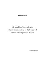
Fig.
9.7.
(Useful heat)/work as a function
of
process steam temperature
(after
Porter
and
Mastanaiah
[2]).
Chapter
9.
The gas turbine as
a
cogeneration (combined heat and power) plant
179
\
U
3
W
I80
Advanced
gas
turbine cycles
production to 35th. Gases leave the exhaust stack at 138°C under maximum load
conditions.
For the first operating condition (HRSG unfired) the heat load is estimated at 7.5 MW.

For the second condition (HRSG fired) when 35
t/h
of saturated steam is raised, the heat
load is 23 MW. The values of heat to work ratios
(AD)
are thus
7.5
(=)
=
2.34, and
($
)
=
7.19, respectively.
Other parameters for the plant operating condition-f HRSG unfired (WHR) and
HRSG fired (WHB)-are as follows:
Alternator power output 3.2
MW
Airmass flow rate 20.45
kg/s
Pressure ratio 7: 1
Maximum temperature 890°C
Thermal efficiency 0.23
Heat recovery steam generator
Unfired Steam (saturated) mass flow rate 12
t/h
Steam pressure 13 bar
Fired Steam (saturated) mass flow rate 35
t/h
Steam pressure 13 bar

WHR WHB
($=
1.34)
A
2.34
7.19
EUF 0.77
0.85
FESR 0.147
O.O75(7C
=
0.4,
VB
=
0.9)
A full description of this plant is given in Ref. [l].
9.6.2.
The Liverpool University CHP plant
A gas turbine CHP scheme which operates at Liverpool University, UK, consists of a
Centrax 4 MW (nominal) gas turbine with an overall efficiency of about 0.27, exhausting
to a WHB. The plant meets a major part of the University’s heat load of about 7 MW on a
mild winter’s day. Supplementary firing of the WHB (to about 15 MW) is possible on a
cold day. Provision
is
also made for by-passing the WHB when the heat load is light, in
spring and autumn,
so
that the plant can operate very flexibly, in three modes viz., power
only, recuperative and supplementary firing.
The major performance parameters at design operating conditions are as follows:

Electrical power output 3.8 MW
Heat output (normal load)
6.6
MW
(with supplementary firing) 15.0
MW
Gas fuel energy supply 14.95 MW
Thermal efficiency 0.27
Chapter
9.
The gas turbine as a cogeneration (combined hear and power) plant
181
Headwork ratio
1.7
Water supply temperature
(TB)
150°C
Water return temperature
(TA)
128°C
Exhaust gas
flow
(MG)
Water
flow
(Mw)
150
t/h
15.3
kgls

0.4
X
0.9
0.27(0.9
+
1.7
X
0.4)
For WHR operation EUF
=
0.73
FESRZ1-
(&G
=
I
.7,
vc
=
0.4,
vc
=
0.9)
=
0.155
A
full
description
of
the economics
of

operating this plant over a complete year is given
by
Horlock
[I].
References
[I
]
Horlock,
J.H. (1997).
Cogeneration-Combined Heat and Power Plants, 2nd edn, Krieger, Malabar, Florida.
[2] Porter,
R.W.
and Mastanaiah,
K.
(1
982),
Thermal-economics analysis
of
heat-matched industrial
cogeneration systems, Energy
7(2).
171
-
187.

Appendix
A
DERIVATION
OF
REQUIRED

COOLING FLOWS
A.1.
Introduction
The stagnation temperature and pressure change in the cooling mixing process have
been shown to be dependent on the cooling air flow
(w,)
as a fraction of the entering gas
flow
(w,),
i.e. on
JI
=
wc/wg.
In this Appendix, an analysis by Holland and Thake
[l],
which allows external film cooling (flow through the blade surface) as well as internal
convective cooling (flow through the internal passages), is summarised (see also Horlock
et al.
[2]
for a full discussion). It is based mainly on the assumption that the external
Stanton number
(Sr,),
which is generally a weak function of the Reynolds number, remains
constant as engine design parameters
(Tco,
and
r)
are changed.
A.2.
Convective cooling only

A
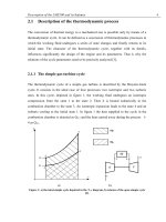
simple heat balance for a typical convectively cooled blade (as illustrated in
Fig. A. 1 a, which shows the notation) is
It is assumed that the temperature of the coolant does not fully reach the temperature of the
metal before it leaves the blade, i.e.
Tc,
<
Thus, the concept of a cooling efficiency is
introduced
so that
The exposed area for heat transfer
(Asg)
is then replaced on the premise that, for a set of
similar gas turbines, there is a reasonably constant ratio between
A,,
and the cross-
sectional area of the main hot gas flow
Axg.
Thus, writing
A,
=
hixg
=
Awg/p,Vg
in
Eq.
(A3) gives
183
184
Advanced gas turbine cycles

(a)
CONVECTIVE COOLING NOTATION
-
%=
hgAsg(Tg-Tbl)
I
wg
+
wc
(b)
FILM COOLING NOTATION
1'
%t
=
'fg
(Taw-
Tbl
)
Fig.
A.
1.
Notation for turbine blade cooling. (a) Convective cooling and
(b)
film
cooling (after Ref.
[2]).
so
that
(WclWg)
=

A(cpg/c,)(hg/cp,pgVg)(T,i
-
TbI)/%ool(Tbl
-
Tci)
=
A(cpg/c,)Sfg(Tgi
-
Tbl)/'?/cooI(Tbl
-
(A41
For
a row in which the blade length is
L,
the blade chord is
c,
the spacing is
s
and the
where
Stg
=
hg/(cpgpgVg)
is the external Stanton number.
flow discharge angle is
a,
the ratio
h
is given approximately by
h

=
A,,/A,,
=
2Lc/(Ls
COS
a)
=
2c/(s
COS
a).
With
s/c
=
0.8
and
a
=
75",
the value of
A
is then about 10. The total cooled surface area
is found to
be
greater than the surface area of the blade profiles alone because of the
presence of cooled end-wall surfaces (adding another
30-40%
of surface area), complex
trailing edges and other cooled components. It would appear from an examination of
practical engines that
h(cpg/c,)

could reasonably
be
given a value of about
20.
Eq.
(A4)
then provides the basic form on which a cooling model can
be
based.
The external Stanton number is assumed not to vary over the range of conditions being
studied. Considering
(cp,/c,)(A,,/A,,)Stg
as a constant
C,
Eq.
(A4)
then becomes
$h
=
Wc/Wg
=
cw+
=
C&"/7)coo,(
1
-
E"),
(A5)
Appendix
A.

Derivation
of
required cooling
Jows
I85
where
w+
is the 'temperature difference ratio' given by
and
eo
is the overall cooling effectiveness, defined as
80
=
(Tgi
-
Tbl)/(Tgi
-
Tci).
Tgi
and
Tci
are usually determined from and/or specified for cycle calculation
so
that the
cooling effectiveness
.zO
implicitly becomes a requirement (subject to
Tbl
which again can
be

assumed for a 'level of technology'). If
r)cool
and
C
are amalgamated into a single
constant
K,
then
(A8)
l+b
=
K&"/(
1
-
Eo),
for convective cooling, as used by El-Masri [3].
A.3.
Film
cooling
The model used by Holland and Thake
[
11
when film cooling is present is indicated in
Fig. A.lb. Cooling air at temperature
Tc,
is discharged into the mainstream through the
holes in the blade surface to
form a cooling film. The heat transferred is now
649)
where

Taw
is the adiabatic wall temperature and
hfg
is the heat transfer coefficient under
film cooling conditions. The film cooling effectiveness is defined
as
('410)
Qnet
=
Asghg(Taw
-
Tbl)
=
Wccpc(Tco
-
Tcih
EF
=
(Tgi
-
Taw>/(Tgi
-
Ted.
Then a new 'temperature difference ratio'
W+
may be written as
w+
=
(Taw
-

Tbl)/(Tco
-
Tci)
=
[EO
-
(1
-
r)cool)&F
-
&O&F~c0011/r)cool(l
-
EO).
('41 1)
It can
be
argued that
cF
should
be
independent of temperature boundary conditions and
It follows from
Eqs.
(A9)
and
(AlO)
that
in the subsequent calculations it is taken as
0.4, based on the experimental data.
l+b

=
(wc/wg>
=
(c,g/c,)(Asgs~,/A,g>~w+,
(A 12)
where
p
=
hfg/[kg(
1
+
B)]
in which
hf,
is the heat transfer coefficient under film cooling
conditions and
B
=
hfgt/k
is the Biot number, which takes account of a thermal barrier
coating (TBC) of thickness
r
and conductivity
k.
In practice,
hfg
increases above h,, and
(1
+
B)

is increased as TBC is added. For the
purposes of cycle calculation,
p
is therefore taken as unity and
l+b
=
cw+,
('41
3)
where
C
is the same constant as that used for convective cooling only.
186
Advanced gas turbine cycles
A.4.
The cooling efficiency
The cooling efficiency can be determined from the internal heat transfer. If
Tbl
is taken
to be more
or
less constant, then it may be shown that
where
6
=
(h,A,/w,c,)
=
(St,A,/A,,),
St,
is now the internal Stanton number, and

A,
and
A,,
refer to surface and cross-sectional areas of the coolant flow.
Experience gives values of
8
for various geometries, but
Sr,
is also a weak function of
Reynolds number and
so,
in practice, there is relatively little variation in cooling efficiency
(0.6
<
cool
<
0.8).
In the cycle calculations described in Chapter 5,
cool
was taken as
0.7,
and assumed to be constant over the range of cooling flows considered.
AS.
Summary
Since ‘open’ film cooling
is
now used in most gas turbines, the form of Eq.
(AI
3)
was

adopted for the cycle calculations of Chapter 5, i.e.
Taking
(cpg/cF)(As,/Ag)
=
20
as representative of modern engine practice, and
Sr,
=
1.5
X
a value of
C
=
0.03
is obtained. The ratio
(cpg/cF)
should then increase
with
Tg (but only by about
8%
over the range
1500-2200K).
This variation was,
therefore, neglected in the cycle calculations described in Chapter
5.
However,
it
was found that the cooling flows calculated from these equations were less
than those used in recent and current practices in which film cooling is employed. This is
for two main reasons:

(i)
designers
are
conservative, and choose to increase the cooling flows
(a) to cope with entry temperature profiles (the maximum temperature being well
above the mean) and local hot spots on the blade and
(b) locally, where cooling can be achieved with relatively small penalty on mixing
loss
(and hence on polytropic efficiency),
so
regions remote from these injection
points are cooled with this low loss air;
(ii) in practice, some surfaces in a turbine blade row will be convectively cooled with no
film cooling. The use of Eq. (A15) with
Eq.
(AI
1)
for the whole blade row assembly
therefore leads to the total cooling flow being underestimated. Film cooling leads to
more efficient cooling, which is reflected in
W+
being much less than
w+;
for the
NGVs
of a modem gas turbine
W+
may take a value of about
2
but

w
+
about 4.
In the calculations described in the main text, allowance was made for such practical
issues by increasing the value of the constants
C
by a ‘safety factor’ of 1.5. Thus, cooling
flows were determined from
Appendix A.
Derivation
of
required cooling
jbws
187
with
w+
=
[EO
-
(1
-
r]cool)&F
-
EOEFr]~ooll/r]cool(~
-
W+
=
[EO
-
0.12

-
0.28~,]/0.7(
I
-
EO).
(A 17)
in which
EF
was taken as
0.4
and
r]cool
as
0.7,
so
that
(A181
In any particular cycle calculation, with the inlet gas temperature
Tg
known together
with the inlet coolant temperature
Tci,
and with an assumed allowable metal temperature
Tbl,
cO
was determined from
Eq.
(A7).
W+
was then obtained

from
Eq.
(A18) and the
cooling flow fraction
$
from
Eq.
(A16).
References
[I]
Holland, M.J. and Thake. T.F.
(1980).
Rotor blade cooling in high pressure turbines, AlAA J. Aircraft 17(6),
[2] Horlock, J.H., Watson, D.E. and Jones, T.V. (2001). Limitations on
gas
turbine performance imposed by
[3] El-Masri, M.A. (1987). Exergy analysis of combined cycles:
Part
1
Air-cooled Brayton-cycle
gas
turbines,
412-418.
large turbine cooling flows, ASME
J.
Engng
Gas
Turbines Power 123(3), 487-494.
ASME J. Engng
Power

Gas Turbines 109.228-235.

Appendix B
ECONOMICS
OF
GAS TURBINE PLANTS
B.l.
Introduction
The simplest way of assessing the economics of a new power plant is to calculate the
unit price of electricity produced by the plant (e.g.
$/kWh)
and compare it with that of a
conventional plant. This is the method adopted by many authors
[1,2].
Other methods
involving net present values may also
be
used
[3,4].
B.2.
Electricity pricing
The method is based on relating electricity price to both the capital related cost and the
03.1)
where
PE
is the annual cost of the electricity produced (e.g.
$
p.a.),
Co
is the capital cost of

plant (e.g.
$),
P(i,N)
is a capital charge factor which is related to the discount rate
(i)
on
capital and the life of the plant
(N
years) (see Section
B.3
below),
M
is the annual cost of
fuel supplied (e.g.
$
p.a.), and
(OM)
is the annual cost
of
operation and maintenance (e.g.
$
p.a.).
recurrent cost of production (fuel and maintenance of plant):
PE
=
Pco
+
M
+
(OM),

The ‘unitised’ production cost (say
$kWh)
for the plant is
pE
PCO
M
(OM)
YE=-=-
+-+-
WH WH WH WH
where
&$/kWh), the rate of supply of energy in the fuel &kW) and the utilisation,
H,
i.e.
is the rating of the plant
(kW)
and
H
is the plant utilisation (hours per annum).
The cost of the fuel
per
annum,
M,
may
be
written as the product of the unit cost of fuel
M
=
lFH.
03.3)

Thus the unitised production cost
is
where
(v0)
=
W/F
is the overall efficiency of the plant. Alternatively, the unit cost of fuel
4‘may
be
written as the cost per unit mass
S
(say $/kg) divided by the calorific value
[CV],
189
190
Advanced
gas
turbine
cycles
(kWh/kg),
so
that
In a comparison between two competitive plants, one may have higher efficiency (and
hence lower fuel cost) but may incur higher capital and maintenance costs. These effects
have to be balanced against each other in the assessment of the relative economic merits of
two plants.
B.3.
The capital charge factor
The capital charge factor
(P)

multiplied by the capital cost of the plant
(CO)
gives the
cost of servicing the total capital required. Suppose the capital costs of a plant at the
beginning of the first year is
CO
and the plant has a life of
N
years
so
an annual amount
must
be
provided which is
(Coi
+
B).
The first term
(COi)
is the simple interest payment
and the second
(B)
matures into the capital repayment after
N
years (i.e. interest added to
the accumulated sum at the end of each year), thus
+(I
+i)+(l+i)2+ +(1+i)N-']=~0,
so
that

C0
i
B=
(1
+i)N
-
1
where it has been assumed that the annual payments are made at the end
of
each year.
Hence the total annual payment is
where the capital charge factor
P
is sometimes referred to as the annuity present worth
factor and is given as
In arriving at an appropriate value of
p,
the choice of interest or discount rate
(i)
is
crucial. It depends on:
the relative values of equity and debt financing;
whether the debt financing is less than the life of the plant;
tax rates and tax allowances (which vary from one country to another);
inflation rates.
In comparing two engineering projects the practice is often to use a 'test discount rate',
applicable to both projects.
An American approach has been outlined by Williams
[l].
He elaborates the simple

expression for
P
to take account of many other factors beyond a simple single interest (or
Appendix
E.
Economics
of
gas
turbine
plants
191
discount) rate. He defines a discount rate as
i
=
‘Yere
+
(1
-
T)(Ydrd,
(B.8)
where
ae,
ad
are the fractions of investment from equity and debt,
re,
rd
are the
corresponding annual rates of return and
T
is the corporate tax rate.

B.4.
Examples
of
electricity pricing
In the unit price of electricity
(YE)
derived in Section
B.2,
the dominant factors are the
capital cost per kilowatt
(Co/m,
which generally decreases inversely as the square root of
the power (i.e. as
Win),
the fuel price
[,
the overall efficiency
T~,
the utilisation
(H
hours
per
year) and to a lesser extent the operational and maintenance costs
(OM).
Fig.
B.
1
shows simply how
YE,
minus the

(OM)/WH
component, varies with
Co/W
and
m,
for
H
=
4ooo
h and
6
=
1
ckwh. Horlock
[4]
has used this type of chart to compare
three lines of development in gas turbine power generation:
(i) a heavy-duty simple cycle gas turbine, of moderate capital cost, with a relatively low
pressure ratio and modest thermal efficiency (e.g.
36%);
(ii) an aero-engine derivative simple cycle gas turbine, usually two-shaft and
of
high
pressure ratio, the capital cost per kilowatt of
this
plant being surprisingly little
different from (i) in spite
of
it being derived
from

developed aero-engines, but
thermal efficiency being slightly higher (e.g.
39%);
(iii) a heavy-duty
CCGT
plant, based on (i), which has a high thermal efficiency but
0
zoo0
4ooo
m
1m
12OOo
14000
18ooo
HEAT RATE
(kJkWh)
Fig.
B.
1.
Electricity price
as
a function
of
capital cost and plant efficiency
(after
Ref.
[4]).
192
Advanced
gas

turbine cycles
Rough locations for types (i), (ii) and (iii) are given in the electricity price charts of
Figs.
B.2
and
B.3;
for
8000
and
4ooo
h utilisation, respectively. For
8000
h, the CCGT
plant type (iii) has a clear advantage in spite of increased capital costs. At
4OOO
h, the
CCGT plant loses this advantage over the aero-engine derivatives because of the increase
in the capital cost element
(H
has been decreased).
However, more direct comparisons should include factors of operation and main-
tenance, the cost of which have been omitted in the presentations of Figs.
B.2
and
B.3.
B.5.
Carbon dioxide production and the effects
of
a carbon
tax

As pointed out in Chapter
7,
the amount of C02 produced by a thermal plant
is
now a
major criterion of its performance, for environmental and therefore economic reasons.
In electrical power stations a new measure of the performance is the amount of C02
produced per unit of electricity generated, i.e.
A
=
kg(C0,)kWh; this quantity can
be
non-dimensionalised by writing
A’
=
A(
16/44)(LCV) where (16/4) is the mass ratio
of
fuel to
C02
for methane and (LCV) in its lower heating value. However, presenting the
plant’s ‘green’ performance in terms of
A
directly allows the cost of any
tax
on the carbon
dioxide to
be
added to the untaxed cost of electricity production most easily.
Fig.

B.4
(after Davidson and Keeley
[5])
shows values of
A
plotted against thermal
efficiency for a high carbon fuel (coal) and a lower carbon fuel (natural gas). It illustrates
that one obvious route towards a desired low production of this greenhouse gas is to seek
high thermal efficiency (another is to
use
lower carbon fuel).
In future, the economics of electric power generation is likely to
be
affected
considerably by the amount of C02 produced and the level of any environmental penalty
8
0
0
2MH)
4000
Boo0
8OOo
lo000
12OOo
14000
18ooo
HEAT
RATE
(kJ/kWh)
Fig.

B.2.
Electricity price
for
typical
gas
turbine plants-running
hours
8000
p.a.
(after
Ref.
[41).
193
0
ZOO0
4000
6OQO
8MH)
loo00 12000
14000
16000
HEAT RATE
(kJ/kWh)
Fig.
B.3.
Electricity price
for
typical gas turbine plants-running hours
4000
p.a. (after Ref.

[4])
imposed by a carbon
or
carbon dioxide tax. For example, a
CCGT
plant
of 54% thermal
efficiency, delivering electricity at
a
generating cost
of 3.6
ckWh can produce
C02
at
a
rate
of
0.3
kg/kWh, as indicated in Fig.
B.5.
If
the carbon dioxide tax
is
set at $50/tonne
of
C02
(5
ckg
C02),
then there

is
an additional amount
of
(0.3
x
5)
=
1.5
ckWh to be
0.2
0.25 0.3 0.35
0.4
Od5
0.5
0.55
0.6 0.65 0.7
OVERALL EFFICIENCY [LHV]
Fig.
B.4.
Carbon dioxide emissions for various power plants
as
a function of overall efficiency (after Davidson
and
Keeley
[5]).
1
94
Advanced
gas
turbine cycles

0 50
loo
150
200
250
CARBON
DIOXIDE
TAX
$/TONNE
Fig. B.S. Effect
of
carbon dioxide tax on electricity price
for
a combined cycle gas turbine plant.
added to the cost
of
generation, making it 5.1 c/kWh. This may make the plant
uneconomic when compared to a nuclear station
or
even windmills. This point is
illustrated in Fig. B.5 which shows how the generation cost for this CCGT plant would
vary with the tax level and how other plants might then come into competition with it.
If
however, the original CCGT plant was modified to reduce the amount
of
C02
entering the atmosphere from the plant (say to
0.15
kg/kWh) at an additional capital cost it
may lead to an increase in the untaxed cost of electricity (say from 3.6 to 4.2 c/kWh).

Then the effect of a carbon dioxide tax of 5 ckwh would
be
to increase the electricity
price to (4.2
+
0.15
X
5)
=
4.95 ckWh and this is below the ‘taxed’ cost of the original
plant. In fact, the new plant would become economic with a carbon dioxide tax
of
T
ckg
C02,
which is given as (3.6
+
T
X
0.3)
=
(4.2
+
T
X
0.
IS), i.e. when
T
=
4

c/kg
C02.
References
11
I
Williams, R.H. (1978). Industrial Cogeneration, Annual Review
of
Energy
3,
313-356.
121
Wunsch,
A.
(1985). Highest efficiencies possible by converting gas turbine plants, Brown Boveri Review
1,
455-456.
I31
Horlock,
J.H.
(1997). Cogeneration-Combined Heat and Power Plants, 2nd edition, Krieger, Malabar,
Florida.
[41 Horlock. J.H. (1997), Aero-engine derivative
gas
turbines for power generation: thermodynamic and
economic perspectives, ASME Journal of Engineering for Gas Turbines and Power
I
19(
I),
119- 123.
[SI

Davidson, B.J. and Keeley, K.R. (1991), The thermodynamics
of
practical combined cycles.
Roc.
Instn.
Mech. Engrs., Conference on Combined Cycle Gas Turbines,
28-SO.
SUBJECT
INDEX
ABB GT24/36 CCGT plant, 128
Absorption, 136- 139
Adiabatic combustion, 23
Adiabatic mixing,
5
I
Adiabatic wall temperature, 185
Advanced steam topping (FAST), 99,
100
Aero-engine derivative, 191
Aftercooler, 94-96
Air recuperation,
90
Air standard cycles, 28, 33, 48, 68
Allowable stack temperature, 118, 174
Ambient temperatures, 13- 14, 24
Annual cost, 189
Annual payments,
190
Annuity present worth factor, 190
Arbitrary overall efficiency, 6-7, 40-42,

66,
Area for heat transfer, 183
Area plots of the range of EUF and
FESR,
179
Artificial efficiency, 170
Arbitrary overall efficiency, 41
Artificial thermal efficiency, 170
112-1 13, 168
Basic power plant, 2
Basic
STIG
plant, 85
Basic gas turbine cycles, 27-46
Beilen CHP plant, 177, 180
Biot number, 185
Bled steam feed water heating,
1
19- 120.
Boiler efficiency,
5,
1
1
I,
I
17
Boiler pressure,
1
18
Boudouard reaction, 143

121
Calculated exergy losses, 83
Calculating plant efficiency, 7
1
-84
Calorific value experiment,
5,
14, 41, 87,
90
Calorific value, 5-6, 14, 41, 87, 90, 189-190
Capital charge factor, 189, 190-191
Capital cost per kilowatt, 191
Capital costs, 131, 132, 189,
190-
192
Carbon dioxide, 131, 192, 193
Carbon dioxide removal, 144-145, 146, 157
Carbon
tax,
163-164, 192-194
Carnot cycle,
7,
8,
9,
20
Carnot efficiency, 7, 9
Carnot engines, 7-9, 16- 17,
20
Cascaded humid air turbine (CHAT) cycle,
101,

102,
104,
107
CBT and CCGT plants with full oxidation,
158
CBT open circuit plant, 39
CCGT (combined cycle gas turbines), xiv, 109,
111,
112, 116, 117, 123
CCGT plant with feed water heating by bled
steam, 119
CCGT plant with
full
oxygenation, 158
Change in overall efficiency, 2
1
-22, 127
Change in total pressure, 62
Centrax 4
MW
gas turbine, 180
CHAT (cascaded humid air turbine) plant,
101,
102,
104,
107
Chemical absorption, 137
Chemical absorption process, 137
Chemical reactions, 22, 141
-

145
Chemically reformed gas turbines (CRGT), 133,
CHP
see
combined heat and power
CHP plant, 3, 167, 174, 177
Classification of gas-fired plants, 132
Classification, gas-fired cycles, 132- 136
Closed circuit gas turbine plant, 2, 4
Closed cyclic power plant,
1
Closed cycles
reforming, 143, 148, 157
147-153
air standard, 33
efficiency, 4-6
exergy flux, 19-22
195
196
Subject
Index
power generation,
I
steady-flow energy equation,
13
C02 produced per unit of electricity, 192
C02 removal at high pressure level, 135
C02 removal at low pressure level,
135
COz removal equipment,

136
Coal fired IGCC,
I
15,
164
Cogeneration plant, 3, 4, 167, 168
Cogeneration plants
see
combined heat and
power plants
Combined cycle gas turbines (CCGT),
109,
Combined heat and power plant, 3, 167, 174,
Combined power plant, 2, 4,
109
Combined STIG cycle,
99
Combined heat and power (CHP) plants
112-129
177
operation ranges, 174- 177
performance criteria, 168-173
power generation,
I
unmatched gas turbines, 173- 174, 175
Combined heat and power (CHP) plants, xi,
Combined plants,
109-
113
efficiency,

11
I
power generation,
1
steam injection turbines, 99
see
also
combined cycle gas turbines;
combined heat and power
167-181
Combustion temperature, 48,
56
Combustion with fuel modification,
160
Combustion with full oxidation, 160
Combustion with recycled flue ga,
144
Combustion with excess air, 141
Combustion
complete,
140-
141
fuel modification, 133, 134, 147-153
open circuit plants, 39-42
oxidant modification, 135, 154-
161
recycled flue gases,
144
temperatures, 47-57, 65-68, 73-81
Combustor outlet temperature, 47

Complete combustion,
140-
141
Completely dead state, 22
Complex cycle with partial oxidation and
reforming, 157
Complex RWI cycles,
105
Component performances, 33-34
Compressor water injection,
101
-
102
Computer calculations, 43-45,65-68,75-81
Constant pressure closed cycle
see
Joule-Brayton cycle
Convective cooling, 7
1
-72, 183
-
185
Conventional power plant,
1
Cool Water IGCC plant, 115
Cool Water pilot plant, 114
Coolant air fractions, 74, 79
Cooled efficiency, 56, 58
Cooling air flow, 183
Cooling

air fractions, 57, 65, 71-84, 184- 187
air-standard cycles, 48-55,
5
I,
54-59
effectiveness, 185
efficiency, 72-73, 183, 186
flow fraction,
60,
65,
187
mixing processes, 183
plant efficiency,
71
-73
reversible cycles, 49-54
thermal efficiency, 47-68
turbine blade rows, 59-65, 186
flows, 47-68,71-73, 183-187
Cooling of internally reversible cycles, 49
Cooling of irreversible cycles, 55
Corporate tax rate, 191
Cost of electricity, 131, 163
CRGT (chemically reformed gas turbines), 133,
Cycle

Costs, 131, 132, 190-192
148-153
analysis parameters, 8-9, 20-21
calculations, 65-68

efficiency
see
thermal efficiency
widening,
9,
2
1
Cycles burning non-carbon fuel (hydrogen),
I52
Cycles with modification
of
the oxidant in
combustion, 154
Cycles with perfect recuperation, 92
Dead state, 15, 22
Debt financing,
190
Delivery work. 22
Demand loads,
170-
173
Derivation of required cooling flows, 183- 187
Design, combined heat and power plants, 177
Development of
the
gas turbine, xi
Dewpoint temperature,
1
14,
I

19. 122
Direct removal of C02, 145
Subject
Index
197
Direct removal, carbon dioxide,
144-
145
Direct water injection cycles, 103
Discount rate,
190-
19
1
Disposal, carbon dioxide, 132
Dry and wet cycles,
104
Dry
efficiency, 94
Dry
recuperative cycles, 91
Dual pressure systems, 121, 123, 129
Dual pressure system with no low pressure water
economiser, 123
Dual pressure system
with
a low pressure
economiser, 123
Economic viability, 163
Economics of a new power plant, 189
Economics, 131, 132, 163-164, 189-194

Economiser water entry temperature,
I
19, 120
Effect of carbon dioxide, 194
Effect of steam air ratio, 89
Effectiveness
(or
thermal ratio), 33
Efficiency, 4
Efficiency
closed circuit plants, 4-6
combined cycle turbines, 126
dry, 94
exhaust heated combined cycles,
1
12-
1
14
fired combined cycle turbines, 116
Joule-Brayton cycle,
I,
3, 9,
IO,
20, 28
maximum, 35,38,66,81, 126
open circuit power plants, 6-7
plants, 7
1
-84
power generation, 9

rational, 6, 22, 24-25
steam injection turbine, 87-89
water injection evaporative turbines, 94-98
see
also
plant efficiency; thermal efficiency
EGT
see
evaporative gas turbines
Electricity pricing, 131, 163-164, 189-192
El-Masri EGT cycles, 96
End
of
pipe C02 removal, 132,
I64
Energy equations, 13, 85, 87, 91, 172
Energy utilisation factor (EUF), 7, 168-169,
Enthalpy, 13- 14, 33-34
changes, 43, 6 1-62
entropy diagrams, 9
1
-92
flux,
13.90
specific, 24
174-177, 178-179
Entropy, 9, 16-17,24,64-65,91-92
Entropy generation, 65
Entry feed water temperature.,
1

19, 120
Equilibrium constants, 143
Equipment to remove carbon dioxide, 132
Equity and debt financing,
I90
EUF
see
energy utilisation factor
Evaporative gas turbines (EGT), 85,9
I
-98,
Exergy flux, 19
Exergy losses, 25, 83
Exergy, 13, 15, 82-83
see
also
temperature-entropy diagrams
99- 102
equation, 23
losses, 83-84, 100-102
flux,
19-21,23,25
Exhaust, 112-14, 116-122, 140-141
Exhaust heated (supplementary fired) CCGT,
1
16
Exhaust heated (unfired) CCGT,
1
I2
Exhaust irreversibility, 14, 19, 83

Exit turbine temperature, 59
External irreversibilities,
8
External Stanton number, 184- 185
Extraction work. 22
FAST cycle, 99, 103
Feed heating, 114, 116, 119-123, 128, 129
Feed water temperature,
1
14, 120, 122, I23
FESR, 171, 172, 173, 174, 176, 177,
180,
181
(FGiTCR) cycle, 152
Film cooling, 72-73, 183, 184, 185
Fired combined cycle gas turbines, 116- 123,
First industrial gas turbine,
xiii
Flows
see
fuel energy saving ratio
see
Flue Gas thermo-chemical recuperation
174-177
cooling, 47-68,7 1-73, 183- I87
mainstream, 71 -72
massflow,42,71-72,
117-118
work, 14-
18

see
also
steady-flow
Flue Gas thermo-chemical recuperation
Fluid mechanics, 59-65
Foster-Pegg plant, 99
Fuel

(FGiTCR), 133, 144-145, 151-153
steam, 119-120,
121
air ratio, 41 -42