Báo cáo y học: "A danger of low copy numbers for inferring incorrect cooperativity degree" pps
Bạn đang xem bản rút gọn của tài liệu. Xem và tải ngay bản đầy đủ của tài liệu tại đây (693.37 KB, 15 trang )
RESEA R C H Open Access
A danger of low copy numbers for inferring
incorrect cooperativity degree
Zoran Konkoli
Correspondence: zorank@chalmers.
se
Chalmers University of Technology,
Department of Microtechnology
and Nanoscience, Bionano Systems
Laboratory, Sweden
Abstract
Background: A dose-response curve depicts the fraction of bound proteins as a
function of unbound ligands. Dose-response curves are used to measure the
cooperativity degree of a ligand binding process. Frequently, the Hill function is used
to fit the experimental data. The Hill function is parameterized by the value of the
dissociation constant and the Hill coefficient, which describes the cooperativity
degree. The use of Hill’s model and the Hill function has been heavily criticised in
this context, predominantly the assumption that all ligand s bind at once, which
resulted in further refinements of the model. In this work, the validity of the Hill
function has been studied from an entirely different point of view. In the limit of low
copy nu mbers the dynamics of the system becomes noisy. The goal was to asses the
validity of the Hill function in this limit, and to see in what ways the effects of the
fluctuations change the form of the dose-response curves.
Results: Dose-response curves were computed taking into account effects of
fluctuations. The effects of fluctuations were described at the lowest order (the
second moment of the particle number distribution) by using the previously
developed Pair Approach Reaction Noise EStimator (PARNES) method. The stationary
state of the system is described by nine equations with nine unknowns. To obtain
fluctuation-corrected dose-response curves the equations have been investigated
numerically.
Conclusions: The Hill function cannot describe dose-response curves in a low
particle limit. First, dose-response curves are not solely parameterized by the
dissociation constant and the Hill coefficient. In general, the shape of a dose-
response curve depends on the variables that describe how an experiment
(ensemble) is designed. Second, dose-response curves are multi-valued in a rather
non-trivial way.
Background
The Hill function is frequently used to infer the degree of cooperativity of the chemical
reaction in which ligand molecules bind to a protein [1]. Often, the binding of a ligand
increases the association rate for the binding of the next ligand. Such reactions are
said to be (positively) cooperative. There are examples of cooperative reactions in cell
biology. The classical example is the binding of oxygen molecules by hemog lobin [1].
Other perhaps less well-known examples would be parts of the Notch signaling and 30
S ribosome assembly processes [2], as well as the assembly of ch olesterol-sphingomye-
lin complexes [3]. Also, the noise characteristics of various ligand binding reactions
Konkoli Theoretical Biology and Medical Modelling 2010, 7:40
/>© 2010 Konkoli; licensee BioMed Central Ltd. This is an Open Access article distributed under the terms of the Creative Commons
Attribution License ( which permits unrestricted use, distribution, and reproduction in
any medium, provided the original work is properly cited.
were studied theoretically in [4] and some of the experimental systems could be classi-
fied as cooperative reactions. A cooperative reaction builds a final complex succes-
sively. If strong cooperativity is present, the dynamics of the system can be studied
using Hill’s model, at least to a first approximation [5].
Hill’s model is a grossly simplified version of reality. The model is constructed by
assuming that binding and unbinding of ligands occur in one step as
ChAC
h0
+↔
(1)
where C
0
denotes a protein that binds ligands A,andC
h
is the ligand-protein com-
plex. The Hill co efficient h describes the number of binding sites on the protein. Both
the forward and the back reactions are allowed.
Strictly speaking, the Hill coefficient in Hill’s model (1) is a stoichiometry coefficient
and should be an integer number larger than zero. H owever, in the calculations that
fol low, h will be allowed non-integer values. Thus in the context of this work the Hill
model should be understood more from a model average perspective, where the Hill
coefficient is an effective parameter.
An important quantity related to Hill’s model is the fraction of the proteins that are
bound
≡
+
c
cc
h
h0
(2)
In particular, the dependence of ’ on the amount of unbound ligand in the system a
is of considerable interes t, and is referred to as a dose-res ponse curve. A function fre-
quentlyusedtofitadose-responsecurveis the expression derived by Hill, the so-
called Hill function, given by
H
h
h
a
a
K
a
K
()=
+1
(3)
where c
0
, c
h
, a are used to denote the amounts of unbound proteins, bound proteins,
and free ligands, respectively. Please note that the Hill function is only parameterized
by K and h. When fitting experimental data to extract K and h, it is useful to allow h
to be a real number. Also, the Hill functio n is used frequently in theoretic al studies to
model cooperativity effects.
In general, c
0
, c
h
and a can denote average particle numbers, particle concentrations
or partial pressures. It really depends on the types of experiments one wishes to
describe. The di ssociation constant is essentiall y controlled by the ratio of the forward
and the backward reaction rates.
The original Hill’s model is unrealistic since a truly multiparticle reaction with a high
Hill’s coefficient would be a very unlikely reaction event. The probability that all
required ligand molecules meet at the right place, at the right time, is very small. The
model was already criticised by Hill himself [6,7]. Subsequently, more realistic models
were suggested in a series of studies: Adair [8]; Monod, Wyman, Changeux [9]; and
Koshland, Nemethy, Filmer [ 10]. The difference between the models was critically
Konkoli Theoretical Biology and Medical Modelling 2010, 7:40
/>Page 2 of 15
investigated on the mean field le vel in [5], which confirmed Hill ’ s original claim that
the Hill equation can be used in a case of strong cooperativity whe n intermediate
states are short-lived. For a reaction set that appears strongly cooperative as in (1), the
Hill coefficient provides a rough measure of the cooperativity degree of the reaction.
Despite the problems discussed above, the use of Hill’s model has some merits [1],
and the Hill equation is used frequently in many fields as discussed in review article
[11]. Accordingly, in this work, H ill’ s model will be taken as a basic standard for
describing multiparticle (cooperative) reactions. The validity of the model has been
extensively investigated previously. The conditions for safe usage of Hill ’s model can
be easily verified.
From now on, it wi ll be assumed that the Hill model u nder investigation is a valid
alias for a more complica ted multiparticle-like reaction scheme. The focus will be on
investigating the correctness of the resulting Hill’sfunction’
H
(a)inalowparticle
number limit. The ultimate goal of this study is to investigate in what ways the effects
of the noise related to the low copy numbers affect the form of the dos e-response
curve predicted by Hill. Please note that such a goal enforces consideration of a closed
system. For an open system, where injection and the decay of particles are allowed,
one cannot use the Hill function at all.
Results and discussion
Model description
The fundamental quantity we wish to understand is the fraction of bound proteins ’
in a situation when particle numbers are low. This is done by considering a closed sys-
tem in a well mixed regime. In such a situation it is sufficient to count the particles. In
the following, n
0
, n
h
, and n
A
will denote the number of C
0
, C
h
, and A particles respec-
tively. A stochastic model will be considered with the forward reaction rate a and the
back reaction rate b. The rates have the dimension of inverse time. Owing to the sto-
chastic nature of the model, the particle numbers will fluctuate. The ensemble averages
of fluctuating quantities will be denoted by 〈.〉. Accordingly, particle amounts will be
expressed in terms of average particle numbers, c
0
= 〈n
0
〉, c
h
= 〈n
h
〉,anda = 〈n
A
〉.In
such a case the dissociation constant in equation (3) is precisely given by
K
h
=
!
(4)
The expression for K in (4) can be obtained from the stationary state equatio ns that
describe the system in the mean field limit. Use of equations (27-29) and (30) in the
methods section leads to the desired result. Strictly speaking, the variable K is not a
dissociation constant, but it can be related to it by trivial rescaling by the volume of
the system.
For any type of initial conditions the dynamical system at hand will reach equili-
brium. The focus will be on investigating the equilibrium state of the model, which in
turn will enable us to compute the dose response curve ’(a).
Analytical description of system is possible
The central technical result of this paper is the derivation of t he nine (non-linear)
equations ( 5-13) with nine unknowns. These equations describe t he equilibrium state
Konkoli Theoretical Biology and Medical Modelling 2010, 7:40
/>Page 3 of 15
of the model. The derivation of the equations is described in the methods section. The
equations can help in analytical understanding of the problem.
The first three stationary state equations are given by
Kc c a
h
h
a
h
aa
h
=
()
00
2
(5)
cc P
h
+=〈〉
00
(6)
ahc L
h
+=〈〉
0
(7)
In equation (5), an d in the followin g, the symbol c with a subscript denotes a corre-
lation function. Correlation functions were introduced previously (Konkoli, Z.: Multi-
particle reaction noise characteristics, submitted) and describe fluctuations. The
situation when all c = 1 corresponds to the mean field limit, where the ef fects of fluc-
tuations are absent. It is easy to see that in such a case equations (5-7) combine to
give the class ical Hill funct ion in ( 3). However, the correlation functions do not equal
one in general, and the expression for the Hill function in equation (3) might be
invalid.
Equations (6) and (7) express the fact that the total number of protein complexes
(with and without ligands) P
0
, and the total number of ligands in the system (both free
and bound) L
0
, cannot change over time. Averages 〈P
0
〉 and 〈L
0
〉 need to be used;
depending on an ensemble, these quantities might be stochastic. It ultimately depends
on how the system is prepared during an experiment.
The remaining six equations feature correlation functions heavily. The first three are
0000ha
h
=
(8)
hh h ha
h
=
0
(9)
ha a aa
h
=
0
(10)
and are obtai ned from analysis of the dynamics that brings the systems to a station-
ary state. The last three equations are the conservation laws that express the fact that
initial fluctuations in P
0
and L
0
cannot change over time:
ahach
Lahc
c
aa h ha hh
h
h
22
0
22
2
2
++=
〈〉−−
(11)
cccc
PP
hh hhh0
2
00 0 0
2
0
2
0
2
++=
〈〉−〈〉
(12)
ca hcc ac hc hh
LP hc
ahhhhah
h
00 0 0
2
00
+++=
〈〉−
(13)
Konkoli Theoretical Biology and Medical Modelling 2010, 7:40
/>Page 4 of 15
The nine equations with the nine unknowns (5-13) are the central result of the
paper. The equations are non-linear and fully describe the stationary state of the sys-
tem when the effects of particle number fluctuations are taken into account. The
observables of interest (average numbers of particles and correlation functions) are
implicit functions of the ensemble properties 〈P
0
〉, 〈L
0
〉,
〈〉P
0
2
,
〈〉L
0
2
, and 〈P
0
L
0
〉.
The equations are not exact. They were derived using the Pair Approach Reaction
Noise Estimator (PARNES) method introduced previously (Konko li, Z.: Multiparticle
reaction noise characteristics, submitted). The PARNES method works by approximat-
ing higher order moments of a part icle number distribution by second order moments.
Should the need arise, the method can be easily extended beyond the pair approach
level.
The PARNES method is based on the usage of correlatio n forms. The correlation
forms are used in studies of spatially extended diffusion controlled reactions [12]. They
are employed to close the hierarchy of many-point density functions. In the present
work, the particular methods discussed in [13] were adopted to study a well mixed
reaction system. Because a second quantization formalism is used, the PARN ES
approximation is naturally expressed as a closure relationship for factorial moments of
a particle number distribution. The implementation of the closure procedure is shown
in the methods section. There are other ways to perform the closure [4,14-18].
Clearly, once moments are given it should be possible to work backwards and extract
the form of the particle number distribution function. This is a rathe r non-trivial pro-
blem and will be studied else-where. Essentially, the PARNES approximation is an
expansion around the P oisson distribution. For c ≈ 1 the distribution function is Pois-
son-like. Situations with c <1andc >1 describe sub- and supra-Poisson regimes
respectively.
The Hill equation is valid for large copy numbers
It is possible to see that when particle numbers become large the correlation functions
approach the mean field limit in which all correlation functions are equal to one. For
example, by neglecting the a-h
2
c
h
, 〈P
0
〉 and hc
h
terms in equations (11), (12) and (13)
respectively, and assuming that
〈〉≈〈〉LL
0
2
0
2
,
〈〉≈〈〉PP
0
2
0
2
and 〈L
0
P
0
〉 ≈ 〈L
0
〉〈P
0
〉,the
resulting equations can be solved by the mean field ansatz. This shows that the Hill
function can be used in a large particle number limit.
A danger of inferring an incorrect Hill’s coefficient
The issue is whether all solutions of the central equation system are such that ’ can
be expressed solely as a function of a. If this is the case then there is only one equa-
tion to use, and there should be no ambiguity regarding the proper choice of Hill’s
coefficient. By inspecting the form of the central equations it can be seen that this is
not the case in general. For example, depending on the procedure used to compute
the points in the plot that depicts ’(a), many curves can be obtained. Equivalently, in
more technical terms, for a given reaction system, repeating the experiment to deter-
mine ’(a) with different ensemble setups (the ways the system is prepared), one can
obtain different curves for ’(a). Fitting the curves to ’
H
(a) would result in different
Hill’s coefficient for each curve. Thus, the fact that the central equations depend on
Konkoli Theoretical Biology and Medical Modelling 2010, 7:40
/>Page 5 of 15
ensemble properties has far reaching consequences when it comes to extractin g the
correct Hill coefficient from experiments.
Numerical tests
The question is how much the effects of noise affect the shape of dose-response
curves. To address this question the nine equations were solved numerically for rela-
tively low copy numbers of the protein that binds ligands. F igures 1 and 2 shown that
’ is not solely a function of a, but depends on the characteristics of the ensemble as
suggested. The figures describe the Poisson and pure ensembles respectively. The
curves in the figures clearly depend on the way that is used to prepare the initial state
of the system.
Analysis of both figures shows that for large particle numbers the mean field result
(the Hill function) is obtained. This is expected, since the mean field description
should be correct for large copy numbers. However, in general, the discrepancy from
the mean field case can be signific ant. For Poisson-like initial conditions the reference
curve is approached from below. In the case of pure initial states, the reference curve
is approached from above (below) for high (low) values of a.
For pure initial states, and in the intermediate regions of a, ’ curves are much stee-
per that the corresponding Hill function. Please note that the curves for pure states are
multi-valued since for a given value of a there can be more than one value of ’ (e . g.
all thin curves in Figure 2 for values of a slightly greater than one are multi-valued).
Similar behaviour is observed for Poisson-like initial states but the onset occurs at
Figure 1 Fraction of bound proteins (Poisson initial state). A dose-response curve (the fraction of the
bound proteins ’ plotted as a function of a) for a Poisson-like ensemble:
〈〉L
0
2
= 〈L
0
〉
2
+ 〈L
0
〉 and
〈〉P
0
2
=
〈P
0
〉
2
+ 〈P
0
〉. Each curve is obtained by varying 〈L
0
〉 for a fixed value of 〈P
0
〉. The thickest full line is the
reference Hill curve ’
H
(a), plotted with K = 1, depicting the mean field limit. The shape of the curve does
not depend on the values of the ensemble parameters 〈L
0
〉 and 〈P
0
〉. The thin curves are fluctuation-
corrected dose-response graphs obtained using the PARNES method. The full line was obtained with 〈P
0
〉 =
1, the dashed line with 〈P
0
〉 = 2, and the dotted line with 〈P
0
〉 = 4. The curves that account for noise (thinner
curves) approach the reference mean field curve from below for large values of 〈P
0
〉 but are distinct
otherwise.
Konkoli Theoretical Biology and Medical Modelling 2010, 7:40
/>Page 6 of 15
smaller values of a (e.g. the dotted line in Figure 1). The question is whether such
behavior is an artefact of using the PARNES approximation.
Figure 3 depict s ’(a) o btained by an exact diagonalisation of the master equation.
The figure shows that ’(a) is indee d multi-valued. The exact solutions exhibit richer
behavior than is predicted by the PARNES method. It is very likely that the erratic
alternation of points has to do with the fact that not all ligands can be fully absorbed
by the receptors. For example, assume that one observes a snapshot of the system
dynamics where all proteins in the system have bound all ligands. If one adds more
ligands to the system, any number in range from 1 to h - 1, exactly that number of
ligands will never be bound by the recep tor proteins. A similar effect was observed in
a related study [19]. Such effects cannot be explained directly by usage of the PARNES
method. The PARNES method can describe such behavior only qualitatively.
Figure 4 depi cts ’ as a function of L
0
for a pure ensemble. From a theoretical point
of view the dependence of ’ on a is of interest, but ’ is more likely to be plotted as a
functi on of L
0
in experimental work. Please note that ’(L
0
) is a single valued fun ction.
However, the curve depicting the exact dependence of ’ on L
0
is not s mooth. The
notion of the curve is t o be understood by interpolating between allowed poin ts since
only integer values for L
0
makesenseforapureensemble.Thecurveobtainedby
using the PARNES approximation follows the exact result much more closely than the
mean field curve.
Conclusions
Many dangers have already been recognized in using the Hill function to fit experi-
mental data. The difficulties discussed so far in the literature are mostly related to the
Figure 2 Fraction of bound proteins (pure initial state). Does response curves for the system prepared
in a pure state:
〈〉=LL
0
2
0
2
and
〈〉=PP
0
2
0
2
The curves were obtained in the same way as for Fig. 1. The
thickest full line is the reference Hill curve obtained with K = 1. Other curves describe the effects of
fluctuations and were obtained using the PARNES method: the full (P
0
= 2), the dashed (P
0
= 3), the
dotted (P
0
= 4), and the dot-dash (P
0
= 8). The thinner curves approach the reference mean field curve for
large values of P
0
. The curves are distinct and their shape depends on the value of P
0
.
Konkoli Theoretical Biology and Medical Modelling 2010, 7:40
/>Page 7 of 15
Figure 3 Fraction of bound proteins (pure initial state), exact result. Exact dose response curves for a
system in pure states. As in Fig. 2 the thickest full line is the reference Hill curve. Thinner curves were
generated by direct diagonalisation of the master equation. The thinner full lines are obtained for fixed
value of P
0
and looping values of L
0
. For each point (L
0
, P
0
) the master equation was solved numerically
and observables of interest were computed. The full line is for P
0
= 2. The dashed line is obtained for a
much larger number of receptors P
0
= 8. This figure shows that exact dose response curves are multi-
valued. Since not all points are physical, the points were connected using linear interpolation to guide the
eye. The dose response curves obtained in such a way are rather erratic. Furthermore, the multi-value
character is not an artefact of using linear interpolation. There are many physical points with nearly
identical values for a having many distinct values for ’.
Figure 4 Fraction of bound proteins; L
0
dependence. The fraction of the bound proteins ’ is plotted
as the function of free ligands in the system L
0
for the pure state. All curves were obtained for P
0
= 2. The
thickest full line is the mean field result. The thinner full line is obtained using the PARNES method. The
dashed curve is obtained by exact diagonalisation of the master equation. Please note that the PARNES
curve (thin full line) agrees best with the exact result (dashed line).
Konkoli Theoretical Biology and Medical Modelling 2010, 7:40
/>Page 8 of 15
fact that the Hill model is only an approximation of a more complicated reaction
scheme. This work points to a yet another danger, but in terms of principles.
The findings of this work point to the fact that one should be careful in using the
Hill function to fit experimental data when the number of particles in the system is
low. The actual dependence of ’ on a is much more complex than predicted by the
Hill function ’
H
(a). First, dose-response curves depend on the way the experiment is
done. Repeating the experiment with different ensemble properties could result in a
number of distinct curves. Accordingly, equally many values for the Hill coefficient
could b e extracted. Second, dose-response curves are multivalued in a rather non-tri-
vial way, which has to do with the fact that some ligands will always be unbound,
depending on the number of ligands in the system.
The discrepancy between fluctuation-corrected dose-response curves and the Hill
function has nothing to with a fundamental flaw in the Hill model itself. The features
are rather generic. Similar behaviour is li kely to be observed for any more realistic
model of ligand binding.
The nine equations obtained in this work could aid experimental studies in which
the Hill coefficient is measured. Clearly, to obtain the correct value for the Hill coeffi-
cient, one needs to use the correct curve. The nine equations that define dose-response
curves could be investigated further to obtain analytical approximations for fluctua-
tion-corrected dose-response curves.
This work can be extended in many ways. The uniqueness conditions for the equa-
tions have not been investigated yet. Preliminary numerical investigations show that
the structure of the solutions is rather complex, since Mathematica so lver had to be
fine-tuned to find the solutions. Also, the nine equations allow for non-physical solu-
tions with negative densities or negative correlation functions. This problem can be
solved by proper parameterization of the densities. The question is whether some o f
the features observed here are an artefact of th e “all or none” reaction principle that is
intrinsic to Hill’s model. For example, it is not clear whether the multi-value character
of dose response curves will still be observed in more realistic ligand binding models.
Some of the issues discussed above will be investigated in forthcoming publications.
Methods
Mapping to quantum field theory
The problem at hand is stochastic and can be described by a master equation:
∂=+
+
⎛
⎝
⎜
⎞
⎠
⎟
+−+
()
++ −+−
t
A
h
Pct n
nh
h
Pc t
nPc
(,) ( ) [ , , ],
()([,,]
0
1
1,,)
(,)
t
n
n
h
nPct
A
h
−
⎛
⎝
⎜
⎞
⎠
⎟
+
⎡
⎣
⎢
⎢
⎤
⎦
⎥
⎥
0
(14)
where ∂
t
denotes the time d erivative, and c =(n
0
, n
h
, n
A
) is a configuration of the
system specified by the number of free proteins, ligand protein-complexes and free
ligands. The states c[+,-, +] and c[-,+,-] are defined by
cnnnh
hA
[, ,] ( , , )±±±= ± ± ±
0
11
(15)
Konkoli Theoretical Biology and Medical Modelling 2010, 7:40
/>Page 9 of 15
where any combination of the plus and the minus signs can be picked at will. The
particle number probability distribution function P(c, t) defines the probability that the
system is foun d in a configuratio n c at a time t. Please note that the equation contains
binomial coefficients that count ways of choosing clusters of h particles.
The quantities of interest are observables of the type
〈〉=
∑
fc fcPct
c
() () (,)
(16)
where f is an arbitrary function of state c. In principle, to compute the averages using
(16) is hard. Such a procedure would require the direct solution of the master equa-
tion, which is computationally rather demandin g. To avoid using equation (16), the
equations of motion for the observables of interest will derived. Once in place, these
equations of motion can be studied directly. To derive the equations, the prob lem is
mapped on to a quantum field theory using the standard techniques [20]. Thereafter, it
is possible to derive the d esired equations of motion in a straig htforward manner.
Please note that any other approach can be used to derive the equations. The filed the-
ory is used in here since it is a useful book-keeping device.
The field theory for the problem is constructed a s follows. The particle number
probability distribution function is used to construct the generating function
|() (,)|
tPctc
c
〉= 〉
∑
(17)
where
|()()()|
^^^
cc c a
n
h
n
n
h
A
〉= 〉
0
0
0
††
†
(18)
and the operators in parentheses denote the creation operators for C
0
, C
h
and A par-
ticles:
ˆ
,
ˆ
††
cc
h0
and â
†
respectively. The operators without the dagger s ign, ĉ
0
, ĉ
h
and â,
denote the corresponding annihilation operato rs. The generating function is the linear
combination of all possible configurations of the system, where each configuration is
weighted by the corresponding probability of occurrence.
The field theory that describes the problem is defined through the expression for the
Hamiltonian operator that describes the dynamics:
−∂ 〉 = 〉
t
tHt|() |()
^
(19)
The requirement for equivalence between equations (14) and (19) fixes the form of
the Hamiltonian operator, which turns out to be
ˆ
ˆ
(
ˆ
)
ˆ
!
ˆˆ ˆ
†† †
Hca c
h
ca c
h
h
h
h
=−
⎡
⎣
⎤
⎦
−
⎛
⎝
⎜
⎞
⎠
⎟
00
(20)
Using quantum field theory formalism, the observable in (16) can be calculated as
〈〉=〈 〉fn n n f
cc cc aa
t
hA
h
h
(, , ) |( , , )|()
^^ ^^ ^^
0
0
0
1
††
†
(21)
Konkoli Theoretical Biology and Medical Modelling 2010, 7:40
/>Page 10 of 15
where the right hand side of equation (21) is evaluated using the standard commuta-
tor rules for the operators
ˆ
,
ˆˆˆˆ
††
cc c cc
00 0 00
1
⎡
⎣
⎤
⎦
=− =
(22)
ˆ
,
ˆˆˆˆˆ
†††
c c cc cc
hh hh hh
⎡
⎣
⎤
⎦
=−=1
(23)
ˆ
,
ˆˆˆˆˆ
†††
aa aa aa
⎡
⎣
⎤
⎦
=−=1
(24)
and the fact that
〈=〈 =〈 =〈11 1 1
0
|| | |
^^^
cca
h
††
†
(25)
Equations of motion
An equation of motion for the observable
ˆ
f
can be derived from
∂〈 〉=−〈 〉
t
ft fHt11||() |[,]|()
^
^
(26)
The equation follows from (19) and the fact that 〈1|
ˆ
H
= 0. In the following, to sim-
plify the notation, an expression of the form
〈〉1| | ( )
^
ft
will be abbreviated to
〈〉
ˆ
f
.
This should cause no confusion between (16) and (21). If the expression contai ns field
theoretic creation and annihilation operators, the expression should be interpreted as
in (21).
Using equ ation (26) with
ˆ
ˆ
,
ˆ
,
ˆ
fcca
h
=
0
it is possible to derive equations of motion for
the average numbers of C
0
, C
h
and A particles given by c
0
= 〈ĉ
0
〉, c
h
= 〈ĉ
h
〉 and a = 〈â〉.
The equations are given by
∂〈 〉=〈 〉
t
c
ˆ
ˆ
0
Ξ
(27)
∂〈 〉=−〈 〉
th
c
ˆ
ˆ
Ξ
(28)
∂〈〉= 〈 〉
t
ah
ˆ
ˆ
Ξ
(29)
where
ˆ
ˆ
!
ˆˆ
Ξ= −
c
h
ca
h
h
0
(30)
Please note that the equations contain the expression 〈ĉ
0
â
h
〉, so it appears that we
need an equation for that quantity as well. This will be dealt with later.
The fluctuations in the numbers of p articles will be described by the second
moments of the particle number distribution for all pairs. The equations for the second
moments are given by
Konkoli Theoretical Biology and Medical Modelling 2010, 7:40
/>Page 11 of 15
∂〈 〉= 〈 〉
t
cc c
ˆˆ ˆ
00 0
2 Ξ
(31)
∂〈 〉=〈 − 〉
th h
cc c c
ˆˆ
(
ˆˆ
)
00
Ξ
(32)
∂〈 〉=〈 + + 〉
t
ca h a hc
ˆˆ
(
ˆˆ
)
00
Ξ
(33)
∂〈 〉=−〈 〉
thh h
cc c
ˆˆ ˆ
2 Ξ
(34)
∂〈 〉=〈 − 〉
th h
ca hc a
ˆˆ
(
ˆˆ
)Ξ
(35)
∂〈 〉=〈 − + 〉
t
aa h h ha
ˆˆ
[( )
ˆ
]12Ξ
(36)
Conservation laws
The system is closed and five conservation laws can be extracted from the equations of
motion. This can be done by taking the appro priate linear combinations of t he equa-
tions so that the time derivatives vanish. The first two conservation laws are given by
〈+〉=〈〉
ˆˆ
cc P
h00
(37)
〈+ 〉=〈 〉
ˆˆ
ahc L
h 0
(38)
and express the fact t hat the total number of protein complexes (with and w ithout
ligands) P
0
, and the total number of ligands in the system (both free and bound) L
0
,
cannot change over time. For example, the first conservation law can be obtained by
adding equations (27) and (28).
Related to the two conservation laws discussed above it is possible to derive the three
additional laws that describe the conservation of fluctuations in P
0
and L
0
:
〈++ + + 〉=〈〉
ˆˆ ˆˆ
(
ˆˆ
)aahachcc L
hhh
222
0
2
2
(39)
〈+ + + +〉=〈〉
ˆˆ ˆˆˆˆ
cc cccc P
hhh0
2
00
2
0
2
2
(40)
〈+ + + +〉=〈 〉
ˆˆ ˆˆ ˆˆ
(
ˆˆ
)cahccachcc PL
hh hh00
2
00
(41)
Please note that the conservation laws involve only quantities that describe the
ensemble that was used t o prepare the system. The ensemble is defined by five inde-
pendent parameters 〈P
0
〉, 〈L
0
〉,
〈〉P
0
2
,
〈〉L
0
2
and 〈P
0
L
0
〉.
Stationary state equations
The Hill function describes stationary states. Accordingly, the equati ons of motion will
be studied in the long time l imit. Re quiring that all time derivatives in equations (27-29)
and (31-36) vanish gives the set of four equations
〈〉=
ˆ
Ξ 0
(42)
Konkoli Theoretical Biology and Medical Modelling 2010, 7:40
/>Page 12 of 15
〈〉=
ˆ
ˆ
c
0
0Ξ
(43)
〈〉=
ˆ
ˆ
c
h
Ξ 0
(44)
〈〉=
ˆ
ˆ
aΞ 0
(45)
The equations involve expressions for which additional equations of motion need to
be derived. Unfortunately, such a procedure results in an infinite hierarchy of equa-
tions. To cut the hierarchy, the PARNES approximation is discussed. In technical
terms, all expressions that involve a product of three of more operators are approxi-
mated by products of the pair co rrelation functions. The pair correlation functions are
defined as
〈〉≡〈〉〈〉
ˆˆ ˆ ˆ
cc c c
00 0 0 00
(46)
〈〉≡〈〉〈〉
ˆˆ ˆ ˆ
cc c c
hhh000
(47)
〈〉≡〈〉〈〉
ˆˆ ˆ ˆ
ca c a
a000
(48)
〈〉≡〈〉〈〉
ˆˆ ˆ ˆ
cc c c
hh h h hh
(49)
〈〉≡〈〉〈〉
ˆˆ ˆ ˆ
ca c a
hhha
(50)
〈〉≡〈〉〈〉
ˆˆ ˆ ˆ
aa a a
aa
(51)
In the s trict mathematical sense the PARNES approximation can be expre ssed as
follows
〈〉≈〈〉〈〉〈〉×
×
()
()
()
ˆˆˆ ˆ ˆ ˆ
cca c c a
x
h
y
zx
h
yz
hh
aa
h
x
x
y
z
00
00
0
2
2
2
χχχχ
yy
a
xz
ha
yz
χχ
0
(52)
where x, y and z are integers greater than or equal to zero. The accuracy of the
PARNES approximation has been investigated on a similar model where it was con-
firmed that it provides a semi-quantitative description (Konkoli, Z.: Multiparticle reac-
tion noise characteristics, submitted). For large particle numbers it is rather accurate.
A similar investigation for Hill’s model (Figure 4) leads to the same conclusions. The
PARNES approximation provides a qualitative d escription of the stationary state of
Hill’s model in the low particle number limit.
Finally, using the PARNES m ethod (52), an approximative form of equations (42-45)
can be derived. Carrying out the procedure, and combining the result with the conser-
vation laws (37-41), results in the nine equations with nine unknowns listed in (5-13),
which were introduced in the results section.
The central equations (5-13) can be obtained roughly as follows. Equation (5) results
from the stationary state condition (42), and equations (6-7) are the first two
Konkoli Theoretical Biology and Medical Modelling 2010, 7:40
/>Page 13 of 15
conservation laws (37) and (38) expressed in a new notation. Equations (8-10) result
from the stationary state conditions (43-45). Equations (11-13) are derived from the
conservation laws for second moments (39-41).
Numerical recipe
In the general case, the equations are rather involved and cannot be solved analytically.
The numerical procedure for solving the equations naturally suggests itse lf as follows.
First, one solves equations (5-7) assum ing that all correlation functions are one. This
gives the first guess for the average particle numbers c
0
, c
h
and a. The values obtained
are inserted into (8-13) to evaluate a guess for the correlation functions. T he resulting
values can be again used again in (5-7) to obtain even better values for the average
particle numbers. The procedure continues until results converge to the fixed point
values.
However, the procedure discussed above is numerically unstable in the low particle
number limit. The plots in the work were generated by a method similar to the analy-
tic continuation. The equations were solved in the large particle number limit by the
method outlined in th e previous paragraph, afte r which the desired point in the
ensemble parameter space can be approached incrementally along a line. In every step,
the solution from the previous point is used as a guess for the point that follows.
Acknowledgements
The financial support of the Chalmers Biocenter and an internal MC2 grant for strategic development is greatly
acknowledged.
Competing interests
The author declares that they have no competing interests.
Received: 23 August 2010 Accepted: 1 November 2010 Published: 1 November 2010
References
1. Ferrell JE Jr: Questions and Answers: Cooperativity. J Biol 2009, 8:157.
2. Williamson JR: Cooperativity in macromolecular assembly. Nature Chem Biol 2008, 4:458-465.
3. Radhakrishnan A, Li XM, Brown RE, Mc-Connell HM: Stoichiometry of cholesterol-sphingomyelin condensed
complexes in mono-layers. Biochim Biophys Acta Biomembranes 2001, 1511:1.
4. Gurevich KG, Agutter PS, Wheatley DN: Stochastic description of the ligand-receptor interaction of biologically
active substances at extremely low doses. Cell Signal 2003, 15:447-453.
5. Weiss JN: The Hill equation revisited: uses and misuses. FASEB J 1997, 11:835-841.
6. Hill AV: The cobinations of haemoglobin with oxygen and with caron monoxide. J Physiol 1910, 40:iv-vii.
7. Hill AV: The Combinations of Haemoglobin with Oxygen and with Carbon Monoxide. I. Biochem J 1913, 7:471-480.
8. Adair G: The Hemoglobin System. VI. The Oxygen Dissociation Curve of Hemoglobin. J Biol Chem 1925, 63:529-545.
9. Monod J, Wyman J, Changeux JP: On nature of allosteric transiitons - a plausible model. J Mol Biol 1965, 12:88-118.
10. Koshland DE, Nemethy G, Filmer D: Comparison of experimental binding data and theoretical models in proteins
containing subunits. Biochemistry 1966, 5:365-382.
11. Goutelle S, Maurin M, Rougier F, Barbaut X, Bourguignon L, Ducher M, Maire P: The Hill equation: a review of its
capabilities in pharmacological modelling. Fundam Clin Pharmacol 2008, 22:633-648.
12. Kotomin E, Kuzovkov V: Modern aspects of diffusion-controlled reactions: cooperative phenomena in bimolecular processes,
Volume 34 of Comprehensive chemical kinetics Amsterdam: Elsevier; 1996.
13. Konkoli Z: Application of Bogolyubov’s theory of weakly nonideal Bose gases to the A+A, A+B, B+B reaction-
diffusion system. Phys Rev E 2004, 69:011106.
14. Elf J, Ehrenberg M: Fast evaluation of fluctuations in biochemical networks with the linear noise approximation.
Genome Res 2003, 13:2475-2484.
15. Gomez-Uribe CA, Verghese GC: Mass fluctuation kinetics: Capturing stochastic effects in systems of chemical
reactions through coupled mean-variance computations. J Chem Phys 2007, 126:024109.
16. Lee CH, Kim KH, Kim P: A moment closure method for stochastic reaction networks. J Chem Phys 2009, 130
:134107.
17. Singh A, Hespanha JP: Lognormal moment closures for biochemical reactions. Proceedings of the 45th Ieee Conference
on Decision and Control, Vols 1-14, IEEE Conference on Decision and Control 2006, 2063-2068.
18. Gillespie CS: Moment-closure approximations for mass-action models. IET Syst Biol 2009, 3:52-58.
19. Konkoli Z: Exact equilibrium-state solution of an intracellular complex formation model: kA ↔ P reaction in a small
volume. Phys Rev E 2010, 82:041922.
Konkoli Theoretical Biology and Medical Modelling 2010, 7:40
/>Page 14 of 15
20. Mattis DC, Glasser ML: The uses of quantum field theory in diffusion-limited reactions. Rev Mod Phys 1998,
70:979-1001.
doi:10.1186/1742-4682-7-40
Cite this article as: Konkoli: A danger of low copy numbers for inferring incorrect cooperativity degree.
Theoretical Biology and Medical Modelling 2010 7:40.
Submit your next manuscript to BioMed Central
and take full advantage of:
• Convenient online submission
• Thorough peer review
• No space constraints or color figure charges
• Immediate publication on acceptance
• Inclusion in PubMed, CAS, Scopus and Google Scholar
• Research which is freely available for redistribution
Submit your manuscript at
www.biomedcentral.com/submit
Konkoli Theoretical Biology and Medical Modelling 2010, 7:40
/>Page 15 of 15