Báo cáo y học: "Theoretical basis to measure the impact of shortlasting control of an infectious disease on the epidemic peak" pps
Bạn đang xem bản rút gọn của tài liệu. Xem và tải ngay bản đầy đủ của tài liệu tại đây (616.43 KB, 21 trang )
RESEARCH Open Access
Theoretical basis to measure the impact of short-
lasting control of an infectious disease on the
epidemic peak
Ryosuke Omori
1,5
, Hiroshi Nishiura
2,3,4*
* Correspondence:
2
PRESTO, Japan Science and
Technology Agency, 4-1-8 Honcho,
Kawaguchi, Saitama 332-0012,
Japan
Abstract
Background: While many pandemic preparedness plans have promoted disease
control effort to lower and delay an epidemic peak, analytical methods for
determining the required control effort and making statistical inferences have yet to
be sought. As a first step to address this issue, we present a theoretical basis on
which to assess the impact of an early intervention on the epidemic peak,
employing a simple epidemic model.
Methods: We focus on estimating the impact of an early control effort (e.g.
unsuccessful containment), assuming that the transmission rate abruptly increases
when control is discontinued. We provide analytical expressions for magnitude and
time of the epidemic peak, employing approximate logistic and logarithmic-form
solutions for the latter. Empirical influenza data (H1N1-2009) in Japan are analyzed to
estimate the effect of the summer holiday period in lowering and delaying the peak
in 2009.
Results: Our model estimates that the epidemic peak of the 2009 pandemic was
delayed for 21 days due to summer holiday. Decline in peak appears to be a
nonlinear function of control-associated reduction in the reproduction number. Peak
delay is shown to critically depend on the fraction of initially immune individuals.
Conclusions: The proposed modeling approaches offer methodological avenues to
assess empirical data and to objectively estimate required control effort to lower and
delay an epidemic peak. Analytical findings support a critical need to conduct
population-wide serological survey as a prior requirement for estimating the time of
peak.
Background
The influenza A (H1N1-2009) pandemic began in early 2009, and rapidly spread
worldwide. Mathematical epidemiologists characterized the epidemic and provided key
insights into its dynamics fro m the earliest stages of the pandemic [1]. The transmis-
sion potential was quantified shortly after the declaration of emergence [2-6], w hile
statistical estimation and relevant discussion of epidemiological determinants were
underway before substantial numbers of cases were reported in many countries [1].
Prior to the pandemic, many countries issued the original pandemic preparedness
plans and guidelines, aiming to instruct the publ ic and to advocate community mitiga-
tion. The goals of the mitigation have been threefold; (a) to delay epidemic peak, (b) to
Omori and Nishiura Theoretical Biology and Medical Modelling 2011, 8:2
/>© 2011 Omori and Nishiura; licensee BioMed Central Ltd. This is an Open Access article distributed under the terms of the Creative
Commons Attribution License ( which permits unrestricted use, distribution, and
reproduction in any medium, provided the original work is properly cited.
reduce peak burden on hospitals and infrastructure (by lowering the h eight of peak)
and (c) to diminish overall morbidity impacts [7]. To assess these aspects under differ-
ent intervention scenarios, various modeling studies have been conducted (e.g. [8-10]),
most notably, by simulating the detailed influenza transmission dynamics.
Although simulations have aided our understanding of expected dynamics in realistic
situations and in different scenarios, analytical methods that objectively determine the
required control effort and that make statistical inference (e.g. evaluation of empirically
observed delay) have yet to be developed. Focus on epidemic peak (relati ng to mitiga-
tion goals (a) and (b) above) has been particularly understudied. Goal (c), on the o ther
hand, is readily formulated in terms of the so-called final epidemic size. The time
delay of a major epidemic (such as that resulting from international border control)
has been explored using simplistic modeling approaches [11,12]; however, the height
and time of an epidemic peak i nvolve nonlinear dynamics, rendering analytical
approaches difficult. De spite the mathematical complexity, goals (a) and (b) can be
more readily understood from empirical data during early epidemic phase than can
goal (c), because an explicit understandi ng of goal (c) in the presence of interventions
requires knowledge of the full epidemiological dynamics over the entire epidemic
period.
In the present study, we present a theoretical b asis from which the impact of an
early intervention on the height and time of epidemic peak may be assessed. As a spe-
cial case, we consider a scenario in which intervention is implemented only briefly dur-
ing the early epidemic phase (e.g. unsuccessful containment). We employ a
parsimonious epidemic model with homogeneously mixing assumption, because non-
linear epidemic dynamics involve a number of analytical complexities. As a first step
towards understanding epidemiological factors that influence the epidemic peak, lead-
ing to the eventual statistical inference of relevant effects, we seek fundamental analyti-
cal strategies to evaluate the impact of short-lasting control on epidemic peak using
the simplest epidemic model [13]. F or our model to become fully applicable and to
more closely match empirical data, a number of extensions are required. We discuss
ways by which these extensions can be practically realized.
Methods
Study motivation
We first present our study motivation. During the early epidemic phase o f the 2009
pandemic, m any countries initially enforced strict countermeasures to locally contain
the epidemic. Early intervention includes, but is not limited to, quarantine, isolation,
contact tracing and school closure. Nevertheless, once it was realized that a ma jor epi-
demic was unavoidable, regions and countries across the world were compelled to
downgrade control policy from containment to mitigation. Although mitigation also
involves various countermeasures (and indeed, mitigation originally intends to achieve
the above mentioned goals (a)-(c)), one desires to know the effectiveness of the unsuc-
cessful containment effort. Among its many outcomes, the present study focuses on
the height and time of epidemic peak.
The applica bility of our theoretical arguments is not restricted to the switch of con-
trol policy. In many Northern hemisphere countries, the start of the major epidemic of
H1N1-2009 (which may or may not have been preceded by early stochastic phase)
Omori and Nishiura Theoretical Biology and Medical Modelling 2011, 8:2
/>Page 2 of 21
corresponds to the summer school holiday period. Adults also take vacation over a
part of this perio d. In addition to strategic school closure as an early countermeasure
against influenza [14,15], school holiday is known to suppress the transmission of
influenza [16], ma inly because transmission tends to be maintained by school-age chil-
dren [2,17-19]. Following this trend, a decline in instantaneous reproduction number
has been empirically observed during the summer holiday period of the 2009 pandemic
[20]. Transmission resumes once a new semester starts. The effecti veness of the sum-
mer holiday period in lowering and delaying the epidemic peak is, therefore, a matter
of great interest.
Both questions are addressed by considering time-dependent increase in the transmis-
sion rate. Let b be the transmission rate per unit time in the absence of an intervention
of interest (or during the mitigation phase in the case of our first question). Due to inter-
vention (or school holiday) in the early epidemic phase, b is initially reduc ed by a factor
a (0 ≤ a ≤ 1) until time t
1
(Figure 1A). Though transmission rate abruptly increases at
time t
1
when the control policy is eased or when the new school semester starts, we
observe a reduced height of, and a time delay in, the epidemic peak compared to the
hypothetical situation in which no intervention takes place (Figure 1B). More realistic
situations may be envisaged (e.g. a more complex step function or seasonality o f trans-
mission), but we restrict ourselves to the simplest scenario in the present study.
Epidemic model
Here we consider the simplest form of Kermack and McKendrick epidemic model [13],
formulated in terms of ordinary differential equations. The following assumptio ns are
made: (i) the population is homogeneously mixing, (ii) the epid emic occurs in a popu-
lation in which the majority of indi viduals are susceptible, (iii) the time scale of the
epidemic is sufficiently shorter than the average life expectancy at birth of the host,
Figure 1 A scenario for t ime-dependent increase in the transmi ssion potential. A. Time dependent
increase in the transmission rate. In the absence of intervention (baseline scenario), the transmission rate is
assumed to be constant b over time. In the presence of early intervention, the transmission rate is reduced
by a factor a (0 ≤ a ≤ 1) over time interval 0 to t
1
. We assume that the product ab ileads to super-critical
level (i.e. aR(0) >1 where R(0) is the reproduction number at time 0), and t
1
occurs before the time at
which peak prevalence of infectious individuals in the absence of intervention is observed. B.A
comparison between two representative epidemic curves (the number of infectious individuals) in a
hypothetical population of 100,000 individuals. R(0) = 1.5, a = 0.90 and t
1
= 50 days. The epidemic peak in
the presence of short-lasting control is delayed, and the height of epidemic curve is slightly reduced,
relative to the case in which control measures are absent.
Omori and Nishiura Theoretical Biology and Medical Modelling 2011, 8:2
/>Page 3 of 21
and we ignore the background demographi c dynamics, (iv) the epidemic occurs in a
closed constant population without immigration and emigration again justified based
on time scale, and (v) once an infected individual recovers, he/she becomes completely
and permanently immune against further infections. Let the numbers of susceptible,
infectious and recovere d individuals at calendar time t be S(t), I(t)andU(t ), respec-
tively. We use the notation U(t)forrecoveredindividualstoavoidconfusionwiththe
instantaneous reproduction number at calendar time t, R(t). The population size N
remains constant over time (N = S(t)+I(t)+U(t)). The so-called SIR (susceptible-
infected-recovered) model is written as
dS t
dt
RtIt
dI t
dt
RtIt It
dU t
dt
It
()
=−
()()
()
=
()()
−
()
()
=
()
,
,
,
(1)
where R(t) is the instantaneous reproduction number (i.e., the average number of
secondary cases generated by a single primary case at calendar time t) and g is the rate
of recovery. Given time-dependent transmission rate b (t) and susceptible population
size S(t) at time t, R(t) is assumed to be given by
Rt
tSt
()
=
()()
.
(2)
Although b(t) will be dealt with as a simple step function in the following analysis,
we use the general notat ion to motivate future analysis of more complex time-d epen-
dent dynamics. We assume that an epidemic starts at time 0 with an initial condition
(S(0), I(0), U(0)) = (S
0
, I
0
,U
0
)whereI
0
=1andU
0
/N ≈ 0, i.e. an epidemic occurs in a
population in which the majority of individuals are susceptible at t =0.Underthis
initial condition, we consider two different scenarios for R(t). First, a hypothetical sce-
nario in which no intervention takes place, i.e.
Rt
St
()
=
()
,
(3)
which is hereafter referr ed to as the baseline scenario. Second, we consider an
observed scenario in which an intervention takes place during the early stage of the
epidemic. Let t
1
and t
m,0
be calendar times at which the intervention terminates, and
at which a peak prevalence of infectious individuals is observed in the absence of inter-
vention, respectively. As mentioned above, we assume that the intervention reduces the
reproduction number by a factor a (0 ≤ a ≤ 1) for 0 ≤ t<t
1
. For t ≥ t
1
,weassume
that the transmission rate is recovered to b as in (3).
Rt
St
tt
St
tt
()
=
()
≤<
()
≥
⎧
⎨
⎪
⎪
⎩
⎪
⎪
for 0
for
1
1
,
.
(4)
We assume t
1
<t
m,0
, i.e. we consider a scenario in which transmission rate recovers
before the time at which peak prevalence is observed in baseline scenario. We further
Omori and Nishiura Theoretical Biology and Medical Modelling 2011, 8:2
/>Page 4 of 21
assume that R(t) >1fort<t
1
. That is, the efficacy a of an intervention effort (or sum-
mer holiday) is by itself not sufficient to contain the epidemic.
To illustrate our modeling approaches, we consider the transmission dynamics of
pandemic influenza (H1N1-20 09), ignoring the detailed epidemiological characteristics
(e.g. pre-existing immunity, realistic distribution of generation time and the presence
of asymptomatic infection). The initial reproduction number in the absence of inter-
ventions R(0) is assumed to be 1.4 [2]. Given that expected values of empirically esti-
mated serial interval ranged from 1.9 to 3.6 days [2,5,21-23], the mean generation time
1/g is assumed to be 3 days [24,25].
Our study questions are twofold. First, we aim to quantify the decline in peak preva-
lence (I(t)/ N) due to a short-lasting interven tion. The peak prevalence of the interven-
tion scenario is always smaller than that of baseline scenario (see below), and we show
that this difference can be analytically expressed. Second, we are interested in the time
delay in observing peak pre valence in the prese nce of intervention. We develop a n
approximate strategy to quantify the difference in times of peak between baseline and
intervention scenarios.
Difference in peak prevalence
We move on to consider estimates of peak prevalence in two scenarios. For mathema-
tical convenience, we use the preva lence of infectious individuals (I(t)/N)toconsider
the epidemic peak. The peak prevalence of infectious individuals is precede d by peak
incidence (gR(t)I (t)/N) by approximately the mean infectious period of 1/g days. As was
realized elsewhere [26], analysis of prevalence is easier than that of incidence. Begin-
ning with two sub-equations of system (1), we have
dI t
dS t R t
()
()
=− +
()
1
1
.
(5)
Note that R(t) is a function of S(t). Integrating (5) in baseline scenario, we obtain
[27]
It I S St
St
S
()
=+−
()
+
()
00
0
ln .
(6)
A theoretical condition for the observation of peak prevalence at time t
m,0
is dI(t
m,0
)/
dt = 0, or equivalently, R(t
m,0
) = 1. As evident from equation (2), this condition satis-
fies S(t
m,0
)=g/b. The peak prevalence I(t
m,0
)/N is then given by [28]
It
N
IS
NN
S
S
RN
R
m,
ln
ln .
0
00 0
0
1
1
0
10
()
=
+
−+
⎛
⎝
⎜
⎞
⎠
⎟
≈−
()
+
()
()
(7)
Note that S
0
/R(0)N represents the proportion yet to be infected and S
0
ln R(0)/R(0)N
is the proportion removed at time t
m,0
. Equation (7) indicates that the peak prevalence
of SIR model is determined by the initial condit ion and the transmission potential R
(0). It should be noted that S
0
/R(0) can be replaced by g/b, and thus, I(t
m,0
) is indepen-
dent of initial condition for U
0
= 0 (a special case).
Omori and Nishiura Theoretical Biology and Medical Modelling 2011, 8:2
/>Page 5 of 21
In the intervention scenario, equation (6) with replacement of b by ab applies for
t<t
1
.
It St I S
St
S
1100
1
0
()
+
()
=++
()
ln ,
(8)
which provides another initial condition at time t = t
1
for t ≥ t
1
. That is, we can also
employ (6) to compute peak prevalence for t ≥ t
1
with initial condition (S(t
1
), I(t
1
),U
(t
1
)). Again, a condition to observe peak prevalence at time t
m,1
is R(t
m,1
)=1,which
gives S (t
m,1
)=g/b. The peak prevalence I(t
m,1
)/N of the intervention scenario is given
by
It
N
It St
NN
St
It St
N
S
m,
ln
1
11 1
11
0
1
()
=
()
+
()
−+
()
⎛
⎝
⎜
⎞
⎠
⎟
=
()
+
()
−
RRN
RSt
S0
1
0
1
0
()
+
()
()
⎛
⎝
⎜
⎞
⎠
⎟
ln .
(9)
Note that R(0) in the above equation refers to bS
0
/g (i.e. we use R(0) in our baseline
scenario to permit an explici t comparison between the two scenarios). Inserting right-
hand side of (8) into (9), we obtain
It
N
IS
N
S
RN
St
S
S
RN
RSt
S
m,
ln ln
1
00 0
1
0
0
1
0
00
1
0
()
=
+
+
()
()
−
()
+
()
()
⎛
⎝
⎜⎜
⎞
⎠
⎟
≈−
()
+
()
+−
⎛
⎝
⎜
⎞
⎠
⎟
()
⎛
⎝
⎜
⎞
⎠
⎟
1
0
101
1
0
1
0
S
RN
R
St
S
ln ln .
(10)
Consequently, relative reduction in p eak prevalence due to intervention within time
t
1
is ε
a
=(I(t
m,0
) -I(t
m,1
))/N, which can be parameterized as
=− −
⎛
⎝
⎜
⎞
⎠
⎟
()
()
1
1
0
0
1
0
S
RN
St
S
ln .
(11)
Equation (11) indicates that the difference of peak prevalence between the two sce-
narios is determined by four different factors; the relative reduction in reproduction
number a due to the intervention, initial condition at time 0, transmission potential R
(0), and fraction of susceptible individuals at time t
1
under the intervention. If the
initial condition, the transmission dynamics in the absence of interventions (i.e. R (0), b
and g) and t
1
are known, an estimate of a gives S(t
1
), yielding an estimate of ε
a
.
Delay in epidemic peak
The time to observe peak prevalence is analytically more challenging than the height of
peak prevalence, because even an approximate estimate requires an analytical solution
to the model (1). We propose a parsimonious approximation strategy w hich leads to
more convenient solutio ns than those discussed in past studies (e.g. [29]). Substituting
I(t) in the first sub-equation of (1) by (1/g)(dU(t)/dt), we have
1
St
dS t
dt
tdUt
dt
()
()
=−
() ()
.
(12)
Omori and Nishiura Theoretical Biology and Medical Modelling 2011, 8:2
/>Page 6 of 21
For the baseline scenario (i.e. b(t)=b), integrating (12) from time 0 to t,
ln .
St
S
Ut U
()
()
=−
()
−
()
()
0
0
(13)
Because U(0)/N ≈ 0,
St S Ut
()
≈
()
−
()
⎛
⎝
⎜
⎞
⎠
⎟
0 exp .
(14)
Subsequently, the third sub-equation of (1) is rewritten as
dU t
dt
NSt Ut
N S Ut Ut
()
=−
()
−
()
()
≈−
()
−
()
⎛
⎝
⎜
⎞
⎠
⎟
−
()
⎛
⎝
⎜
⎞
⎠
⎟
,
exp0
(15)
Here we impose another key approximation. Because the quantity bU(t)/g (≈ R(0)U
(t)/N)forinfluenza(e.g.R(0) = 1.4) tends to be smaller than 1 (especially, before
observing epidemic peak), we use a Taylor series expansion, i.e.,
exp .−
()()
⎛
⎝
⎜
⎞
⎠
⎟
≈−
()()
+
()()
⎛
⎝
⎜
⎞
⎠
⎟
RUt
S
RUt
S
RUt
S
0
1
01
2
0
000
2
(16)
If the quadratic approximation is inadequate for large R(0), a higher order Taylor
polynomial function can be used. Inserting the quadratic approximation into (15), and
imposing a further approximation (i.e. S
0
≈ N), we obtain
dU t
dt
NS
RUt
S
RUt
S
Ut
()
≈−
()
−
()()
+
()()
⎛
⎝
⎜
⎞
⎠
⎟
⎛
⎝
⎜
⎜
⎞
⎠
⎟
⎟
−
01
01
2
0
00
2
(()
⎛
⎝
⎜
⎜
⎞
⎠
⎟
⎟
≈
()
−
()
()
−
()
()
−
()
()
⎛
⎝
⎜
⎜
⎞
⎠
⎟
⎟
,
,
RUt
R
SR
Ut01 1
0
201
2
0
(17)
which appears to be a logistic equation. We use this logistic-form solution instead of
the more commonly employed hyperbolic-form solution [29,30], to illustrate a simpler
approximate solution and to demo nstrate the problem underlying both solutions.
Later, we use a more formal solution (of logarithm ic-form) in the intervention sce-
nario, which is numerically identical to the classical hyperbolic-form solution (see
below). Assuming that U(0) = U
0
>0, the analytical solution of (17) is
Ut
URt
UR
SR
Rt
()
≈
()
−
()
()
+
()
()
−
()
()
−
()
()
−
0
0
2
0
01
1
0
201
01
exp
exp
11
⎡
⎣
⎤
⎦
.
(18)
The derivative of (18) is dU(t)/dt = gI(t). It follows that
It
UR
UR
SR
Rt
()
≈
()
−
()
−
()
()
−
()
⎛
⎝
⎜
⎜
⎞
⎠
⎟
⎟
()
−
()
()
0
0
2
0
011
0
201
01exp
UUR
SR
Rt
0
2
0
2
0
201
01 11
()
()
−
()
()
−
()
()
−
⎡
⎣
⎤
⎦
+
⎡
⎣
⎢
⎢
⎤
⎦
⎥
⎥
exp
(19)
Omori and Nishiura Theoretical Biology and Medical Modelling 2011, 8:2
/>Page 7 of 21
Further differentiation of (19) gives dI(t)/dt, and letting dI(t)/dt = 0, the time to
observe peak prevalence is analytically derived. For the logistic equation, the corre-
sponding time has been referred to as the inflection point of the cumulative curve in
equation (18) [31]. The inflection point t
m,0
to observe peak prevalence is
t
R
SR
UR
m,
ln ,
0
0
0
2
1
01
201
0
1=
()
−
()
()
−
()
()
−
⎛
⎝
⎜
⎜
⎞
⎠
⎟
⎟
(20)
which depends on initial condition and transmission characteristics. In the interven -
tion scenario (in which intervention is short-lasting), an identical approach can be
taken for t<t
1
,replacingb by ab (or by replacing R(0) by aR(0)). Subsequently, the
epidemic peak occurs at t
m,1
(>t
1
). We take a similar approach to that used in (15)
with a computed initial condition (S(t
1
), I(t
1
), U(t
1
)) using (18) and (19). For t ≥ t
1
,
dU t
dt
NSt Ut Ut Ut
()
=−
()
−
()
−
()
()
⎛
⎝
⎜
⎞
⎠
⎟
−
()
⎡
⎣
⎢
⎤
⎦
⎥
11
exp ,
(21)
Now we apply an approximation
exp −
()
−
()
()
⎛
⎝
⎜
⎞
⎠
⎟
≈−
()
()
−
()
()
+
() ()
−
Ut Ut
R
S
Ut Ut
RUtU
1
0
1
1
01
2
0
tt
S
1
0
2
()
()
⎛
⎝
⎜
⎜
⎞
⎠
⎟
⎟
.
(22)
It should be noted that, in the above approximation, we include the term exp(bU(t
1
)/
g), because U(t) -U(t
1
) better satisfies the Taylor series approximation than expanding
U(t) alone. Let constants A, B and C be
ANSt
RStUt
S
RStUt
S
B
=−
()
−
()
()()
−
()
()()
⎛
⎝
⎜
⎜
⎞
⎠
⎟
⎟
1
11
0
2
11
2
0
2
00
2
,
==
()
()
+
()
()()
−
⎛
⎝
⎜
⎜
⎞
⎠
⎟
⎟
=
()
()
RSt
S
RStUt
S
C
St
R
S
00
1
2
0
1
0
2
11
0
2
1
,
00
2
⎛
⎝
⎜
⎞
⎠
⎟
.
(23)
Given these constants, we consider
dV z
dz
ABVz CVz
()
=+
()
−
()
2
,
(24)
where z = t-t
1
and V (z)=U(z + t
1
) for t ≥ t
1
. The initial condition V (0) is V
0
= U
(t
1
). Writing (24) in integral form, we have [30]
1
2
0
0
ABVCV
dV dz
z
V
V
+−
=
∫∫
.
(25)
Past studies have typically assumed hyperbolic-form functions for the analytical solu-
tion of (25) [29,30]. However, we express the solution in logarithmic-form [31,32],
because logarithmic functions are compatible with spreadsheet programs. The logarith-
mic-form solution reads
Vz
XB YXB Xz
CY Xz
()
=
+
()
−−
()
−
()
+−
()
()
exp
exp
,
21
(26)
Omori and Nishiura Theoretical Biology and Medical Modelling 2011, 8:2
/>Page 8 of 21
where
XB AC=+
2
4.
(27)
Also,
Y
XB CV
XB CV
=
+−
−+
2
2
0
0
.
(28)
Differentiating (26) with respect to z an d taking dV (z)/dz = 0, we find the inflection
point z
m,1
to be
z
X
Y
m,
ln .
1
1
=
(29)
Replacing z by t, we obtain
tt
BAC
XB CUt
XB CUt
m,
ln ,
11
2
1
1
1
4
2
2
=+
+
+−
()
−+
()
(30)
as an approximate solution of the epidemic peak in interventio n scenario. The time
delay of this peak, imposed by the intervention in the early epidemic phase, τ
a
is subse-
quently calculated as
=−tt
mm,,
,
10
(31)
using (20) a nd (30) for the right-hand side. The delay depends on initial condition
U
0
, the length of intervention t
1
(both of which are apparent from (20) and (30)) and
on the efficacy of intervention a (since this quantity influences the initial condition U
(t
1
) in (30)).
Application and illustration
Empirical analysis of influenza A (H1N1-2009)
Here, we apply the above described theory to empirical influenza A (H1N1-2009) data.
Figure 2 shows the estimated number of influenza cases based on national sentinel sur-
veillance in Japan from week 31 (week ending 2 August) 2009 to week 13 (week ending
28 March) 2010. The estimates follow an extrapolation of the notifie d number of cases
from a total of 4800 randomly sampled sentinel hospitals to the actual total number of
medical facilities in Japan. The cases represent patients who sought medical attendance
and who have met the following criteria, (a) acute course of illness (sudden onset), (b)
fever greater than 38.0°C, (c) cough, sputum or breathlessness (symptoms of upper
respiratory tract infection) and (d) general fatigue, or who were strongly suspected of
the disease undertaking laboratory diagnosis (e.g. rapid diagnosti c testing). Altho ugh
the estimates of sentinel surveillance data involve various epidemiological biases and
errors, we ignore these issues in the present study. Prior to week 31, the number of
cases was small and the dynamics in the early stochastic phase have been examined
elsewhere [17]. We arbitrarily assume that the major epidemic starts in week 31.
It is interesting to observe that the period A in Figure 2 corresponds to that of sum-
mer school holiday. Due to reporting delay of approximately 1 week [17], we assume
Omori and Nishiura Theoretical Biology and Medical Modelling 2011, 8:2
/>Page 9 of 21
that weeks 31 to 36 inclusive (the latter of which ends on 6 September) reflect the
transmission dynamics during the summer school holiday. Subsequently, school opens
in September with an epidemic peak in late November (period B), followed by abrupt
decline during the winter holiday (period C) and start of winter semester (period D).
Among these periods, we focus on the impact of summer holiday (period A), relative
to period B, in lowering epidemic peak and delaying the time to observe the peak.
More specifically, we estimate the reproduction number R(0) and its reduction a from
the data set encompassing weeks 31 to 42. To permit an explicit estimation, we
assume that linear approximat ion holds, as was similarly assumed elsewhere [15]. We
assume that the reproduction number is reduced by a factor a from week 31 to 36
due to summer holiday, while the reproduct ion number recovers to R(0)fromweek
37 to 42.
Let r
0
be the exponential growth rate of cases per day in the absence of summer
holiday. Because our SIR model approximates the generation time by an exponential
distribution with mean 1/g days, the estimator of R(0) is [33,34]
Rr
ˆ
()
ˆ
/.01
0
=+
(32)
Throughout the summer holiday, we assume that the reproduction number is
reduced to R
A
= aR(0). That is, the growth rate during the summer holiday, r
1
,is
defined by
rr
10
1=+ −
()
.
(33)
Figure 2 Estimated weekly incidence of influenza cases in Japan from 2009-10.Theestimatesare
based on nationwide sentinel surveillance, covering the period from week 31 in 2009 to week 13 in 2010.
The estimate follows an extrapolation of the notified number of cases from a total of 4800 randomly
sampled sentinel hospitals to the total number of medical facilities in Japan. The case refers to influenza-
like illness cases with medical attendance, possibly involving other diseases, but with influenza A (H1N1-
2009) dominant among the isolated influenza viruses during the period of interest. Period A corresponds
to summer school holiday, followed by autumn semester (period B). Period C covers winter holiday and
period D corresponds to winter semester.
Omori and Nishiura Theoretical Biology and Medical Modelling 2011, 8:2
/>Page 10 of 21
Let the weekly incidence be J
k
in week k. During summer holiday period, the condi-
tionally expected value of J
k+1
given J
k
is
E JJ rtJ
rtJ
kk k
k
+
()
=Δ
()
=+−
()
()
Δ
⎡
⎣
⎤
⎦
11
0
1
;exp ,
exp ,
(34)
where Δt is the length of reporting (i.e. 7 days). In week 37, the conditional expecta-
tion is
E JJ
rrt
r
rt
rt
J
r
kk k+
()
=
Δ
()
Δ
()
−
Δ
()
−
=
+−
1
11
0
0
1
0
1
1
1
;
exp
exp
exp
,
(()
)
+−
()
()
Δ
⎡
⎣
⎤
⎦
(
Δ
()
−
+−
()
()
Δ
⎡
⎣
exp
exp
exp
rt
r
rt
rt
0
0
0
0
1
1
1
⎤⎤
⎦
−1
J
k
,
(35)
because, with an initial incidence i
k
in week k, we have
E Ji rtdt
i
r
rt
kk
k
t
()
=
()
=Δ
()
−
()
Δ
∫
exp exp ,
1
1
0
1
1
(36)
and
E Jirt rtdt
irt
r
rt
kk
k
t
+
Δ
()
=Δ
()
()
=
Δ
()
Δ
()
−
∫
11 0
1
0
0
0
1exp exp
exp
exp
(()
.
(37)
See [35] for more details regarding the derivation of (35), which has been applied to
influenza A (H1N1-2009) in other settings [36]. From week 38 to 42, E(J
k+1
; J
k
) simpli-
fies to
Eexp
1
(;) ().JJ rtJ
kk k+
=
0
Δ
(38)
Although adding the information of test negative individuals could potentially yield a
less biased estimate of r
0
[37], we do not have access to this data and so we disregard
this issue for now. Assuming that the observed counts of cases are Poisson distributed
within each period, the likelihood function to estimate r
0
and a is
Lr
JJ JJ
J
kk
J
kk
k
k
k
0
11
32
42
,;
; exp ;
!
J
()
=
()
−
()
()
−−
=
∏
EE
(39)
The maximum likelihood estimates of r
0
and a are obtained by minimizing the nega-
tive logarithm of (39), and the 95% confidence intervals (CI) are computed by profile
likelihood. From the maximum likelihood estimates, we compute the differences in
peak prevalence and times to observe the peak between baseline and second scenarios
using the SIR model (1). For simplicity, we adopt (S
0
, I
0
, U
0
) = (99998, 1, 1) for the
numerical computation and t
1
is assumed to be 50 days (roughly corresponding to the
length of period A plus 8 days).
Although our model (1) adopts exponentially distributed generation time, we can
partiall y address the uncert ainty of r
0
and a in the parametric assumption of the gen-
eration time. That is, we adopt co nstant generation t ime (i.e. delta function) as an
alternative assumption, which is known to yield a theoretical maximum reproduction
Omori and Nishiura Theoretical Biology and Medical Modelling 2011, 8:2
/>Page 11 of 21
number, given identical r
0
and mean generation time [34]. Given r
0
, the esti mator of R
(0) with constant generation time of 1/g days reads
R
r
ˆ
( ) exp
ˆ
.0
0
=
⎛
⎝
⎜
⎞
⎠
⎟
(40)
As mentioned above, the reproduction number during summer holiday reduces to
R
A
= aR(0). Accordingly, the growth rate during the summer holiday, r
1
is written as
rr
10
=+
ln .
(41)
Using the above mentioned likelihood (39) and replacing r
1
of exponential assump-
tion by (41), we estimate r
0
and a. It should be noted that the difference between (33)
and (41) indicates that the estimates of both r
0
and a depend on the realistic distribu-
tion of the generation time [25].
Sensitivity analysis
In addit ion to the analysis of empirical data, we a lso examine sensitivity of the height
and time of peak prevalence to different values of a and t
1
by numerical simulation.
As mentioned above, influenza is our case study, an d the default value of R(0) of base-
line scenario is 1.4, but we also consider R(0) of 1.2 and 1.6. These ranges are adopted,
additiona lly, because we impose an approximation (16). When obtaining the numerical
solutions, initial condition is fixed at (S
0
, I
0
, U
0
) = (99998, 1, 1) for clarity. U
0
=1is
adopted to prevent U
0
= 0 in (18) and in later equations, and also to select a positive
integer value closest to 0 such that U
0
/N ≈ 0.
Results
Influenza A (H1N1-2009)
Figure 3A compares observed and predicted numbers of influenza cases in Japan from
week 31 to 42. Grey bars represent conditionally expected values during summer holi-
day, and white bars represent the expected values during autumn semester. The esti-
mated growth rate in the absence of summer holiday, r
0
is 0.048 (95% CI: 0.029, 0.066)
per day. Thus, the estimated reproduction number R(0) is 1.14 (95% CI: 1.09, 1.20)
which is likely an underestimate (see below).
The estimated relative proportion of the reproduction number under mitigation con-
ditions a is 0.948 (95% CI: 0.842, 1.053). Although t he confidence limits of a include
1, our argument adopts linear dynamics for longer than 10 weeks (note that the largest
number of notifications is seen in week 48), and thus, the reproduction number is con-
servatively estimated (i.e. over the time period that we examine, the transmission
dynamics may become nonlinear); therefore, R(0) is likely underestimated due to the
linear approximation adopted in our quantitative illustration). Thus, we believe it is
appropriate to regard the reduction in the reproduction number during summer holi-
day as marginally significant. The estimat ed reproducti on number during scho ol holi-
day is 1.08.
Even adopting constant generation time of 3 days, r
0
is of a similar order, i.e. 0.048
(95% CI: 0 .029, 0.066) per day. Th e reproduction number R(0), however, is slightly
greater (1.15 (95% CI: 1.09, 1.22)) due to its estimator, exp(r
0
/g). a is estimated at
0.942 (95% CI: 0.832, 1.061).
Omori and Nishiura Theoretical Biology and Medical Modelling 2011, 8:2
/>Page 12 of 21
Figure 3B illustrates the number of infectious individuals in a hypothetical population
with 100,000 individuals using the estimated a and R(0). In the absence o f summer
holiday, the ep idemic peak w ould have been observed at Day 171 with I(t
m,0
)=822
cases. In the presence of summer holiday from time 0 to t
1
, the peak is delayed to Day
192 w ith I(t
m,1
) = 820 cases. Thus, the estimated a and R(0) do not significantly alter
the height of peak prevalenc e when the effects of summer holiday are included (a dif-
ference between the two scenarios of o nly 2 cases), but the delay effect between the
scenarios is as long as 21 days. We do not use our approximate formula for the esti-
mation of time delay in this empirical case study (for reasons explained below).
Because R(0) = 1.14 in the absence of intervention, a major e pidemic can occur when
the initial condition U
0
/N is smaller than 1 - 1/a R(0) = 7.4% of the population.
Assuming a fixed I
0
=1,andvaryingS
0
and U
0
from N - 1 to 0.926N and from 0 to
0.074N, respectively, only slight variations in the reduction of peak prevalence (not
greater than 1 case) are observed, but the time delay varies greatly; under a scenario
with aR(0) ≈ 1orwithS
0
= 0.926N and U
0
=0.074N, a possible maximum delay of
t
1
= 50 days can be readily envisaged.
Differential peak prevalence
Figure 4A examines the sensit ivity of relative peak prevalence to a (i.e. reduction in R
(0)) for assumed R(0) of 1.2, 1.4 and 1.6. Because aR(0) <1 prevents major epidemic
during the early epidemic phase, possible ranges of a satisfying aR(0) ≥ 1varywithR
(0). It is worth noting t hat the relative reductioninpeakprevalenceisanonlinear
function of a. Largest reduction occurs when a lies within the range 0.90 to 0.95,
rather than when a is minimum. Figure 4B examines the sensitivity of relative reduc-
tion in the peak prevalence as a function of the time length of interven tion t
1
(e.g. the
time required to switch control policy from containment to mitigation). Again, to
Figure 3 The impact of summer holiday on the transmission dynamics of influenza A (H1N1-2009).
A. Comparison of the observed and predicted weekly counts of the estimated number of influenza cases
in Japan from week 31 to 42. Grey bars are conditionally expected values during the summer school
holiday, while white bars are the conditionally expected values during autumn semester. B. Numerical
solutions of the number of infectious individuals in a hypothetical population of 100,000 individuals with
initial condition (S
0
, I
0
, U
0
) = (99998, 1, 1). Baseline scenario is compared against intervention scenario
under a short-lasting intervention. For both scenarios, assumed R(0) and mean generation time are 1.14
and 3 days, respectively. In the second scenario, the transmission rate is reduced by a factor a = 0.948 due
to summer school holiday from time 0 to t
1
(=50 days). Although heights of peak prevalence do not
greatly differ from each other, the time to observe the peak is clearly delayed in the second scenario.
Omori and Nishiura Theoretical Biology and Medical Modelling 2011, 8:2
/>Page 13 of 21
satisfy t
1
<t
m,0
, possible ranges of t
1
vary with R(0). The interpretation of Figure 4B is
more straightforward than that of Figure 4A. Essentiall y, the longer the time period of
intervention, the larger the potential reduction of prevalence.
The nonlinear relationship observed in Figure 4A can be explored by combining (11)
with approximate solutions. First, because S(t
1
) ≈ S(0) exp (-a R(0) U( t
1
)/S
0
) in the pre-
sence of intervention, equation (11) can be expressed in the form
=−
()
()
1
1
Ut
N
.
(42)
Second, using an approximate solution of U(t
1
) based on logistic equation (18),
≈
−
() ()
−
()
()
(
+
()
()
()
−
()
101
0
201
01
0
2
0
URt
N
UR N
SR
exp
exp
RRt01 1
1
()
−
()
()
−
⎡
⎣
⎤
⎦
,
(43)
which is a nonlinear function of a. Although the calculation is not shown here due
to its mathematical complexity and lack of practic al interpretation, the derivative of
(43) with respect to a reveals an optimal a yielding the longest delay in Figure 4A.
Delay in epidemic peak
Figure 5A compares epidemic curves of infectious individuals in the absence of interven-
tion between explicit numerical and approximate solutions (i.e. solutions to (1) and (19),
respectively). The height of epidemic peak is approximated well for smaller R(0), reflect-
ing the fact that Tay lor series expansion is a good approximation to the exponential
function. The relationship between R(0) and approximation of epidemic peak height is
also analytically expressed. Inserting (20) into (19), the approximate peak prevalence is
It
SR
R
approx m,
.
0
0
2
01
20
()
=
()
−
()
()
(44)
Figure 4 Sensit ivity analysis of peak prevalence to the effica cy and length of int ervention. A.
Sensitivity of relative peak prevalence of infectious individuals to reduction in the reproduction number, a.
The vertical axis represents I(t
m,1
)/I(t
m,0
), where I(t
m,0
) and I(t
m,1
) represent the peak prevalence in the
absence and presence of intervention, respectively. The time length of intervention, t
1
is fixed at Day 50. B.
Sensitivity of relative peak prevalence of infectious individuals to the time length of the intervention, t
1
. a
is fixed at 0.90. For both panels, the lines are truncated to satisfy aR(0) ≥ 1 and t
1
<t
m,0
where t
m,0
is the
time to observe peak prevalence in the absence of intervention.
Omori and Nishiura Theoretical Biology and Medical Modelling 2011, 8:2
/>Page 14 of 21
It should be noted that S
0
/R(0) can be replaced by g/b, and thus, the peak prevalence
in the approximated logistic form is independent of the initial condition (indeed, the
derivative of a logistic equation is known not to depend on initial condition but rath er
on the carrying capacity [31]). On the other hand, an explicit solution can depend on
initial condition for U(0) >0, i.e.,
It N U R
m,
ln .
00
10
()
=−
()
−+
()
()
(45)
These two quantities are identical for R(0 ) = 1, N ≈ S
0
and U
0
/N ≈ 0. Otherwise,
numerical observation shows that I(t
m,0
) >I
approx
(t
m,0
)forR(0) >1andU
0
/N ≈ 0.
Thus, the smaller the R(0), the better the approximate height of epidemic curve.
While interpretation of the height of peak prevalence is overall straightforward, t he
time to observe peak prevalence is better captured for larger R(0) (Figure 5A). Clearly,
the logistic equation applied to R(0) = 1.2 yields a considerably biased (delayed) time
to observation of epidemic peak (with bias longer than 20 days), and thus, we did not
apply our approximate solution to the above mentioned case study of influenza A
(H1N1-2009). It must be noted that the relationship between R (0) and approximation
of epidemic peak in Figure 5A is regulated not only by R(0) but also by the initial con-
dition U
0
in (20); that i s, the good agreement of the time of peak between two solu-
tions for R(0) = 1.6 is not only due to R(0) but also to U
0
= 1 in our simulation
setting. For suitable values of U
0
, good appro ximations to the time of pea k are
obtained even for R(0) = 1.2 or smaller (results not shown).
Figure 5B compares the estimated time delay in epidemic peak, induced by an early
intervention, between explicit numerical and approx imate solutions. For all three R(0)
that we investigate, approximation methods result in underestimation of the delay (31).
For R(0) = 1.6, the approximate estimate of delay is crudely realized, and its sensitivity
to a is close to that of the explicit numerical solution. The approximation is worst for
R(0) = 1.2 , for which a negative result was yielded for large a.Thesefindingsarein
Figure 5 Assessing approximation of time to observe epidemic peak. A. Comparison of epidemic
curves in the absence of intervention between explicit numerical and approximate solutions. The
population size is assumed to be 100,000 with initial condition (S
0
, I
0
, U
0
) = (99998, 1, 1). The generation
time is exponentially distributed with mean 1/g = 3 days. B. Comparison of estimated delay in epidemic
peak (imposed by a short-lasting intervention) between explicit numerical and approximate solutions. The
assumed length of intervention t
1
is 50 days.
Omori and Nishiura Theoretical Biology and Medical Modelling 2011, 8:2
/>Page 15 of 21
concordance with Figure 5A. It should be remembered that approximation of time of
epidemic peak can vary with initial condition U
0
, indicating that the estimation
requires knowledge of U
0
in addition to R(0) and a (also, as we have seen, good
approximation depends on judicious choice of R(0) and U
0
).
Discussion
In the present study, we have presented fundamental ideas t o assess the impact of a
short-lasting intervention of an infectious disease on the epidemic peak. As a first
step towards explicit evaluation of control effort in lowering and delaying the epi-
demic peak, we comprehensively described analytical expressions for the difference
in the height of, and the time delay in, theepidemicpeakgainedbyintervention,
employing a parsimonious homogenous mixing epidemic model. We restricted our
focus to a simple step function (Figure 1A) which adequately illustrated the role of
summer holiday in lowering and delaying epidemic peak during the influenza
(H1N1-2009) pandemic. Our methods show that both the height and the time of
epidemic peak can be readily controlled by varying initial conditions at a given point
of time at which transmission rate abruptly changes. The proposed method can be
extended in future to encompass more realis tic multiple steps for th e transmission
rate. Analytical solution of the simplest form of Kermack and McKendrick model
has been undertaken multiple times, and is documented in many key references
[27,29-32,38,39] including the original study in 1 927 [13]. However, to our knowl-
edge, the present study is the first to offer a theoretical basis on which to assess the
impact of an early countermeasure on the epidemic peak employing logistic and
logarithmic-form solutions, with a goal to making statistical inferences in the future.
In addition, our analytical expressions not only promote epidemiological understand-
ing of epidemic peak traits, but can be worked backwards to determine required
control effort to achieve desired goals of height and delay of the epidemic peak.
Although manual adjustment of the efficacy of intervention is not practically feasible,
our demonstration of a nonlinear relationship between a and decline in the height of
epidemic peak should be considered a key issue for optimal intervention manage-
ment during an early epidemic phase.
Although public health guidelines have tended to advocate control policy switches
from containment to mitigation at some point in time, the likely impact of unsuccess-
ful containment to epidemic dynamics has been seldom discussed. Indeed, common
illustration o f mitigation (embodied in the three distinct goals (a)-(c) described in the
Background section) do not account for the time-dependent transmission rate (rather,
a guideline illustrates only differential peaks with various reproduction numbers R(0)
[7]). Statistical modeling studies tend to focus only on time-dependent decreases in
transmission potential, with a focus on the instantaneous reproduction number R(t) <1
to demonstrate successful control of an infectious disease (e.g. [40-42]). Motivated by
these problems, we considered the impact of upward change in the transmission rate
during the course of an epidemic. In our case study of influen za H1N1-2009, it was
shown that summer vacation did not appreciably lower the height of an epidemic
peak, but imposed a substantial time delay. Alt hough our approximat e estimation of
the delay in epidemic peak was biased t owards certain choices of R(0) and the initial
number of immune individuals U
0
, this does not imply failure of the model. Rather, by
Omori and Nishiura Theoretical Biology and Medical Modelling 2011, 8:2
/>Page 16 of 21
means of approximate analytical computation, we have shown in (20) and (30) that the
time of epidemic peak critically depends on the fraction of initially immune individuals
prio r to an epidemic. Although a preceding study instead emphas ized the dependence
of the time of p eak on initial number of infectious individuals [32], other studies with
hyperbolic-form s olutions emphasize dependency of the time of peak on U
0
[27,31].
We believe that U
0
is more easily quantified than the initial number of infectious indi-
viduals I
0
in practical settings. The critical importance of the initial number of immune
individuals U
0
is especially highlighted in the influenza A (H1N1-2009) pandemic
because of pre-existing immunity [43-46]. Our analytical undertakings indicate that
statistical inference of t he time delay gained by early control effort will greatly benefit
from population-wide seroepidemiological survey. Depending on the quality of approx-
imation for a given combination of R(0) and U
0
, one can then decide whether the esti-
mation of delay should be based on analytical or numerical solution.
Despite our motivation to eventually offer a method to estimate the impact of an
early intervention, it should be note d that the present study does not account for
uncertainty (e.g. confidence interval) . Our arguments are based solely on deterministic
models, whereas an explicit derivation of the confidence interval requires use of a sto-
chastic Markov jump process [47]. Moreover, potential model extensions are numer-
ous. Relevant factors include, but are not limited to, mobility of host, spatial dynamics,
class-age st ructure (e.g. infection-age dependency), chronological age-structure, social
contact patterns, seasonality, strain specificity and immunological dynamics. All of
these features would increase the realism, but would greatly complicate analytical
inspection, of the model. To illustrate the way forward, we discuss the simplest exam-
ple of a class-age structured model in the Appendix.
Despite many future tasks to be completed, and our realization that the epidemic
peak is vulnerable to heterogeneous patterns of transmission, relevant statistical assess-
ment (including the estimation of R(0), generation time, and incubation period) always
starts with a homogeneous modeling assumption [11,21,23,33,34,48,49]. This is particu-
larly true during the early epidemic phase of a pandemic. In this sense, we believe that
the present study has successfully offered a methodological avenue to statistically
assess empirical data and to assess required control effort to lower and delay epidemic
peak.
Conclusions
This study has presented a theoretical basis on which to assess the impact of short-
lasting intervention on the epidemic peak of an infectious disease. Employing a homo-
geneously mixing epidemic model, we deriv ed analytical expressions for the decline in
the height of epidemic peak and for t he time delay of the peak. Empirical influenza A
(H1N1-2009) data w ere analyzed using a simplistic but practically accessible model,
which estimated that the epidemic peak was delayed for 21 days by the summer holi-
day period in 2009. Approximate logarithmic form solution of the time of epidemic
peak appeared to critically depend on initial condition of immune individuals, support-
ing a need to conduct population-wide serological survey. Despite obvious needs to
address various types of heterogeneity, our framework offers a successful methodologi-
cal avenue to assess relevant empirical data and to advocate requ ired contro l effort to
lower and delay epidemic peak.
Omori and Nishiura Theoretical Biology and Medical Modelling 2011, 8:2
/>Page 17 of 21
Appendix: A way forward
In realistic situations, there is a time delay for newly infected individuals to acquire
infectiousnes s, known as the latent period. This delay is captured by employing the so-
called SEIR (susceptible-exposed-infected-recovered) model. In addition to S(t), I(t)
and U(t), we consider infected but non-infectious individuals E(t). Assuming that the
mean latent period is 1/δ days, the model is written as
dS t
dt
StIt
dE t
dt
StIt Et
dI t
dt
Et
()
=−
()()
()
=
()()
−
()
()
=
()
−
,
,
IIt
dU t
dt
It
()
()
=
()
,
.
(46)
In considering the height of epidemic peak of this system, an equation similar to (6 )
is derived by employing a Lyapunov function, W(S, E, I) [50]. A different derivation is
given elsewhere [51].
WSEI S S E I, , exp .
()
=++
()
−
⎛
⎝
⎜
⎞
⎠
⎟
(47)
The Lyapunov function is known t o yield a constant solution (for any t), thus,
dW/dt = 0. This is confirmed by
dW S E I
dt
W
S
dS
dt
W
E
dE
dt
W
I
dI
dt
,,
.
()
=
∂
∂
+
∂
∂
+
∂
∂
= 0
(48)
At an epidemic peak at time t
m
(where we have dE/dt = dI/dt = 0), two obvious con-
ditions apply,
St
m
()
=
,
(49)
Et It
mm
()
=
()
.
(50)
Using Lyapunov function in (47), we have
WSt Et It WS E I
mmm
()()()
()
=
() () ()
()
,, ,,.000
(51)
Writing both sides of (51) in terms of (47), and taking logarithm of both sides, we obtain
−
()
+
()
+
()
+
()
=−
()
+
()
+
()
+
()
ln ln .St St Et It S S E I
mmmm
0000
(52)
Rearranging (52) leads us to
100010+
⎛
⎝
⎜
⎞
⎠
⎟
()
=
()
+
()
+
()
−+
()
()
It S E I R
m
ln ,
(53)
Omori and Nishiura Theoretical Biology and Medical Modelling 2011, 8:2
/>Page 18 of 21
which is very close to (6). By varying initial conditions at each time point when a
change in transmission rate occurs, equation (53) permits us to measure the impact of
public health intervention on the epidemic peak, under the SEIR assumption. Regard-
ing the time of epidemic peak, a straightforward extension of (15) applies, although the
analytical solution may be rather complex or may not exist. We have
dU t
dt
NSt Et Ut
()
=−
()
−
()
−
()
()
.
(54)
S(t) can be replaced as for (14). Expres sing E(t) as a function of U(t) requires strong
mathematical suppo rts. The problem may be addressed in different ways, but we first
consider an analytical solution of dE/dt, i.e.,
Et E t t S d
t
( ) exp( ) exp( ) exp( )( ( )) ,=
()
−+ − −
∫
0
0
(55)
where
S()
in the right-hand side is eq uivalent to dS/ds for which the derivative of
approximation (15) can be used. We have yet to d erive a simple analytical solution of
the time of epidemic peak from (54), but the above discussion demonstrates that it is
at least possible to compute the height of epidemic peak with more E compartments
(as was discussed in [52]), using our proposed Lyapunov approach. Nevertheless, it
should be remembered that the presence of infection-age dependency in the infectious-
ness profile is likely to complicate the computation of epidemic peak [53]. The incor-
poration of other realistic features, however, is greatly aided by the Lyapunov
approach. In further studies, we will address epidemic peak with seasonality and age-
dependent heterogeneity and in a multi-strain system.
Acknowledgements
We would like to thank three anonymous reviewers for helpful comments on earlier draft of this paper. HN is
supported by the Japan Science and Technology Agency PRESTO program. RO is financially supported by Research
Fellowship of Japan Society for the Promotion of Science.
Author details
1
Department of Biology, Faculty of Sciences, Kyushu University, 6-10 -1 Hakozaki, Higashi-ku, Fukuoka 812-8581, Japan.
2
PRESTO, Japan Science and Technology Agency, 4-1-8 Honcho, Kawaguchi, Saitama 332-0012, Japan.
3
Theoretical
Epidemiology, University of Utrecht, Yalelaan 7, Utrecht, 3584 CL, The Netherlands.
4
School of Public Health, The
University of Hong Kong, Pokfulam, Hong Kong Special Administrative Region, PR China.
5
Centre for Infectious
Diseases, University of Edinburgh, Kings Buildings, West Mains Road, Edinburgh EH9 3JT, UK.
Authors’ contributions
HN conceived of the study, developed methodological ideas and implemented mathematical and statistical analyses.
RO revised analytical results. HN drafted the manuscript and RO and HN discussed and revised the manuscript. All
authors read and approved the final manuscript.
Competing interests
The authors declare that they have no competing interests.
Received: 17 November 2010 Accepted: 26 January 2011 Published: 26 January 2011
References
1. World Health Organization: Mathematical modelling of the pandemic H1N1 2009. Wkly Epidemiol Rec 2009,
84:341-348.
2. Fraser C, Donnelly CA, Cauchemez S, Hanage WP, Van Kerkhove MD, Hollingsworth TD, Griffin J, Baggaley RF,
Jenkins HE, Lyons EJ, Jombart T, Hinsley WR, Grassly NC, Balloux F, Ghani AC, Ferguson NM, Rambaut A, Pybus OG,
Lopez-Gatell H, Alpuche-Aranda CM, Chapela IB, Zavala EP, Guevara DM, Checchi F, Garcia E, Hugonnet S, Roth C, WHO
Rapid Pandemic Assessment Collaboration: Pandemic potential of a strain of influenza A (H1N1): early findings.
Science 2009, 324:1557-1661.
Omori and Nishiura Theoretical Biology and Medical Modelling 2011, 8:2
/>Page 19 of 21
3. Boelle PY, Bernillon P, Desenclos JC: A preliminary estimation of the reproduction ratio for new influenza A(H1N1)
from the outbreak in Mexico, March-April 2009. Euro Surveill 2009, 14, pii:19205.
4. Nishiura H, Castillo-Chavez C, Safan M, Chowell G: Transmission potential of the new influenza A(H1N1) virus and its
age-specificity in Japan. Euro Surveill 2009, 14, pii:19227.
5. McBryde E, Bergeri I, van Gemert C, Rotty J, Headley E, Simpson K, Lester R, Hellard M, Fielding J: Early transmission
characteristics of influenza A(H1N1)v in Australia: Victorian state, 16 May - 3 June 2009. Euro Surveill 2009, 14,
pii:19363.
6. White LF, Wallinga J, Finelli L, Reed C, Riley S, Lipsitch M, M P: Estimation of the reproductive number and the serial
interval in early phase of the 2009 influenza A/H1N1 pandemic in the USA. Influenza Other Respi Viruses 2009,
3:267-276.
7. Department of Health and Human Services, Centers for Disease Control and Prevention: Interim Pre-pandemic Planning
Guidance: Community Strategy for Pandemic Influenza Mitigation in the United States. Early, Targeted, Layered Use of
Nonpharmaceutical Interventions Washington, D.C.: Department of Health and Human Services; 2007.
8. Ferguson NM, Cummings DA, Fraser C, Cajka JC, Cooley PC, Burke DS: Strategies for mitigating an influenza
pandemic. Nature 2006, 442:448-452.
9. Halder N, Kelso JK, Milne GJ: Analysis of the effectiveness of interventions used during the 2009 A/H1N1 influenza
pandemi. BMC Public Health 2010, 10:168.
10. Lipsitch M, Cohen T, Murray M, Levin BR: Antiviral resistance and the control of pandemic influenza. PLoS Med 2007,
4:e15.
11. Scalia-Tomba G, Wallinga J: A simple explanation for the low impact of border control as a countermeasure to the
spread of an infectious disease. Math Biosci 2008, 214:70-72.
12. Cowling BJ, Lau LL, Wu P, Wong HW, Fang VJ, Riley S, Nishiura H: Entry screening to delay local transmission of 2009
pandemic influenza A (H1N1). BMC Infect Dis 2010, 10:82.
13. Kermack WO, McKendrick AG: Contributions to the mathematical theory of epidemics. I. Proc R Soc Ser A 1927,
115:700-721, (reprinted in Bull Math Biol 1991, 115: 33-55).
14. Cauchemez S, Ferguson NM, Wachtel C, Tegnell A, Saour G, Duncan B, Nicoll A: Closure of schools during an
influenza pandemic. Lancet Infect Dis 2009, 9:473-481.
15. Wu JT, Cowling BJ, Lau EH, Ip DK, Ho LM, Tsang T, Chuang SK, Leung PY, Lo SV, Liu SH, Riley S: School closure and
mitigation of pandemic (H1N1) 2009, Hong Kong. Emerg Infect Dis 2010, 16:538-541.
16. Cauchemez S, Valleron AJ, Boelle PY, Flahault A, Ferguson NM: Estimating the impact of school closure on influenza
transmission from Sentinel data. Nature 2008, 452:750-754.
17. Nishiura H, Chowell G, Safan M, Castillo-Chavez C: Pros and cons of estimating the reproduction number from early
epidemic growth rate of influenza A (H1N1) 2009. Theor Biol Med Model 2010, 7:1.
18. Nishiura H: Travel and age of influenza A (H1N1) 2009 virus infection.
J Travel Med 2010, 17:269-270.
19.
Nishiura H, Cook AR, Cowling BJ: Assortativity and the probability of epidemic extinction: A case study of pandemic
influenza A (H1N1-2009). Interdiscip Perspect Infect Dis 2011, 2011:Article ID 194507.
20. Cowling BJ, Lau MS, Ho LM, Chuang SK, Tsang T, Liu SH, Leung PY, Lo SV, Lau EH: The effective reproduction number
of pandemic influenza: prospective estimation. Epidemiology 2010, 21:842-846.
21. Lessler J, Reich NG, Cummings DA, New York City Department of Health and Mental Hygiene Swine Influenza
Investigation Team, Nair HP, Jordan HT, Thompson N: Outbreak of 2009 pandemic influenza A (H1N1) at a New York
City school. N Engl J Med 2009, 361:2628-2636.
22. Cauchemez S, Donnelly CA, Reed C, Ghani AC, Fraser C, Kent CK, Finelli L, Ferguson NM: Household transmission of
2009 pandemic influenza A (H1N1) virus in the United States. N Engl J Med 2009, 361:2619-2627.
23. Cowling BJ, Fang VJ, Riley S, Malik Peiris JS, Leung G M: Estimation of the serial interval of influenza. Epidemiology
2009, 20:344-347.
24. Nishiura H: Time variations in the transmissibility of pandemic influenza in Prussia, Germany, from 1918-19. Theor
Biol Med Model 2007, 4:20.
25. Nishiura H: Time variations in the generation time of an infectious disease: Implications for sampling to
appropriately quantify transmission potential. Math Biosci Eng 2010, 7:851-869.
26. Pitzer VE, Lipsitch M: Exploring the relationship between incidence and the average age of infection during
seasonal epidemics. J Theor Biol 2009, 260:175-185.
27. Bailey NTJ: Macro-modelling and prediction of epidemic spread at community level. Math Modelling 1986, 7:689-717.
28. Brauer F, Castillo-Chavez C: Mathematical Models in Population Biology and Epidemiology New York: Springer; 2000.
29. Bailey NTJ: The Mathematical Theory of Infectious Diseases and Its Applications. 2 edition. London: Griffin; 1975.
30. Kendall DG: Deterministic and stochastic epidemics in closed populations. In Proceedings of the Third Berkeley
Symposium on Mathematical Statistics and Probability. Volume 4. Edited by: Neyman J. Berkeley: University of California
Press; 1956:149-165.
31. Banks RB: Growth and Diffusion Phenomena: Mathematical Frameworks and Applications New York: Springer; 1991.
32. Risch H: An approximate solution for the standard deterministic epidemic model. Math Biosci 1983, 63:1-8.
33. Wallinga J, Lipsitch M: How generation intervals shape the relationship between growth rates and reproductive
numbers. Proc R Soc Lond Ser B 2007, 274:599-604.
34. Roberts MG, Heesterbeek JA: Model-consistent estimation of the basic reproduction number from the incidence of
an emerging infection. J Math Biol 2007, 55:803-816.
35. Nishiura H, Chowell G, Heesterbeek H, Wallinga J:
The ideal reporting interval for an epidemic to objectively
interpret
the epidemiological time course. J R Soc Interface 2010, 7:297-307.
36. Lessler J, Santos TD, Aguilera X, Brookmeyer R, PAHO Influenza Technical Working Group, Cummings DA: H1N1pdm in
the Americas. Epidemics 2010, 2:132-138.
37. Nishiura H: Joint quantification of transmission dynamics and diagnostic accuracy applied to influenza. Math Biosci
Eng 2011, 8:49-64.
38. Nishiura H: Lessons from previous predictions of HIV/AIDS in the United States and Japan: epidemiologic models
and policy formulation. Epidemiol Perspect Innov 2007, 4:3.
39. Dietz K: Epidemics: the fitting of the first dynamic models to data. J Contemp Math Anal 2009, 44:97-104.
Omori and Nishiura Theoretical Biology and Medical Modelling 2011, 8:2
/>Page 20 of 21
40. Nishiura H, Satou K: Potential effectiveness of public health interventions during the equine influenza outbreak in
racehorse facilities in Japan, 2007. Transbound Emerg Dis 2010, 57:162-170.
41. Heijne JC, Teunis P, Morroy G, Wijkmans C, Oostveen S, Duizer E, Kretzschmar M, Wallinga J: Enhanced hygiene
measures and norovirus transmission during an outbreak. Emerg Infect Dis 2009, 15:24-30.
42. Nishiura H, Omori R: An epidemiological analysis of the foot-and-mouth disease epidemic in Miyazaki, Japan, 2010.
Transbound Emerg Dis 2010, 57:396-403.
43. Reichert T, Chowell G, Nishiura H, Christensen RA, McCullers JA: Does Glycosylation as a modifier of Original
Antigenic Sin explain the case age distribution and unusual toxicity in pandemic novel H1N1 influenza? BMC Infect
Dis 2010, 10:5.
44. Itoh Y, Shinya K, Kiso M, Watanabe T, Sakoda Y, Hatta M, Muramoto Y, Tamura D, Sakai-Tagawa Y, Noda T, Sakabe S,
Imai M, Hatta Y, Watanabe S, Li C, Yamada S, Fujii K, Murakami S, Imai H, Kakugawa S, Ito M, Takano R, Iwatsuki-
Horimoto K, Shimojima M, Horimoto T, Goto H, Takahashi K, Makino A, Ishigaki H, Nakayama M, Okamatsu M,
Takahashi K, Warshauer D, Shult PA, Saito R, Suzuki H, Furuta Y, Yamashita M, Mitamura K, Nakano K, Nakamura M,
Brockman-Schneider R, Mitamura H, Yamazaki M, Sugaya N, Suresh M, Ozawa M, Neumann G, Gern J, Kida H,
Ogasawara K, Kawaoka Y: In vitro and in vivo characterization of new swine-origin H1N1 influenza viruses. Nature
2009, 460:1021-1025.
45. Greenbaum JA, Kotturi MF, Kim Y, Oseroff C, Vaughan K, Salimi N, Vita R, Ponomarenko J, Scheuermann RH, Sette A,
Peters B: Pre-existing immunity against swine-origin H1N1 influenza viruses in the general human population. Proc
Natl Acad Sci USA 2009, 106:20365-20370.
46. Igarashi M, Ito K, Yoshida R, Tomabechi D, Kida H, Takada A: Predicting the antigenic structure of the pandemic
(H1N1) 2009 influenza virus hemagglutinin. PLoS One 2010, 5:e8553.
47. Andersson H, Britton T: Stochastic Epidemic Models and Their Statistical Analysis New York: Springer; 2000.
48. Vynnycky E, Trindall A, Mangtani P: Estimates of the reproduction numbers of Spanish influenza using morbidity
data. Int J Epidemiol 2007, 36:881-889.
49. Nishiura H, Inaba H: Estimation of the incubation period of influenza A (H1N1-2009) among imported cases:
Addressing censoring using outbreak data at the origin of importation. J Theor Biol 2011, 272:123-130.
50. Vincent TL, Grantham WJ: Nonlinear and Optimal Control Systems New York: Wiley-Interscience; 1997.
51. Feng Z: Final and peak epidemic sizes for SEIR models with quarantine and isolation. Math Biosci Eng 2007,
4:675-686.
52. Wearing HJ, Rohani P, Keeling MJ: Appropriate models for the management of infectious diseases. PLoS Med 2005,
2:e174.
53. Rost G: SEIR epidemiological model with varying infectivity and infinite delay. Math Biosci Eng 2008, 5:389-402.
doi:10.1186/1742-4682-8-2
Cite this article as: Omori and Nishiura: Theoretical basis to measure the impact of short-lasting control of an
infectious disease on the epidemic peak. Theoretical Biology and Med ical Modelling 2011 8:2.
Submit your next manuscript to BioMed Central
and take full advantage of:
• Convenient online submission
• Thorough peer review
• No space constraints or color figure charges
• Immediate publication on acceptance
• Inclusion in PubMed, CAS, Scopus and Google Scholar
• Research which is freely available for redistribution
Submit your manuscript at
www.biomedcentral.com/submit
Omori and Nishiura Theoretical Biology and Medical Modelling 2011, 8:2
/>Page 21 of 21