Báo cáo y học: " Review and application of group theory to molecular systems biology" ppsx
Bạn đang xem bản rút gọn của tài liệu. Xem và tải ngay bản đầy đủ của tài liệu tại đây (1.45 MB, 29 trang )
REVIEW Open Access
Review and application of group theory to
molecular systems biology
Edward A Rietman
1,2,6
, Robert L Karp
3
and Jack A Tuszynski
4,5*
* Correspondence: jackt@ualberta.
ca
4
Department of Experimental
Oncology, Cross Cancer Institute,
11560 University Avenue,
Edmonton, AB, T6G 1Z2, Canada
Full list of author information is
available at the end of the article
Abstract
In this paper we provide a review of selected mathematical ideas that can help us
better understand the boundary between living and non-living systems. We focus on
group theory and abstract algebra applied to molecular systems biology. Throughout
this paper we briefly describe possible open problems. In connection with the
genetic code we propose that it may be possible to use perturbation theory to
explore the adjacent possibilities in the 64-dimensional space-time manifold of the
evolving genome.
With regards to algebraic graph theory, there are several minor open problems we
discuss. In relation to network dynamics and groupoid formalism we suggest that
the network graph might not be the main focus for understanding the phenotype
but rather the phase space of the network dynamics. We show a simple case of a C
6
network and its phase space network. We envision that the molecular network of a
cell is actually a complex network of hypercycles and feedback circuits that could be
better represented in a higher-dimensional space. We conjecture that targeting
nodes in the molecular network that have key roles in the phase space, as revealed
by analysis of the automorphism decomposition, might be a better way to drug
discovery and treatment of can cer.
1. Introduction
In 1944 Erwin Schrödinger published a series of lectures in What is Life? [1]. Thi s small
book was a major inspiration for a generation of physicists to enter microbiology and
biochemistry, with the goal of attempting to define life by means of physics and chemis-
try. Though an enormous amount of work has been done, our understanding of “Life
Itself” [2] is still incomplete. For example, the standard way in which biology textbooks
list the necessary characteristics of life–in order to delineate it from nonliving matter–
includes metabolism, self-maintenance, duplication involving genetic material and evo-
lution by natural selection. This largely descriptive approach does not address the real
complexity of organisms, the dynamical character of ecological systems, or the question
of how the phenotype emerges from the genotype (e.g., for disease processes [3]).
The universe can be viewed as a large Riemann ian resonator in which evolution takes
place thr ough energy dispersal processes and entropy reduction. Life can b e thought of
as some of the machinery the universe uses to diminish energy gradients [4]. This evolu-
tion consists of a step-b y-step symmetry breaking process, in which the energy densit y
difference relative to the surrounding is diminished. When the uni verse w as formed via
the Big Bang 13.7 billion years ago, a series of spontaneous symmetry-breaking events
Rietman et al. Theoretical Biology and Medical Modelling 2011, 8:21
/>© 2011 Rietman et al; licensee BioMed Central Ltd. This is an Open Access article distributed under the terms of the Creative Commons
Attribution License ( which permits unrestricted use, distribution, and reproduction in
any medium, provided the original work is properly cited.
took place, which evolved the uniform quantum vacuum into the heterogenous structure
we observe today. In fact the quantum fluctuations of the early universe got blown up to
cosmological scales, through a process known as cosmic inflation, and the remnants of
these quantum fluctuations can be observed directly in the variation of the cosmic
microwave background radiation in different directions. At each stage along the evolu-
tion of the universe–from quantum gravity, to fundamental particles, atoms, the first
stars, galaxies, planets–there was a further breaking of symmetry. These cosmological,
stellar, and atomic particle abstractions can be powerfully expressed in terms of group
theory [5].
It also turns out that the very foundation of all of modern physics is based on group
theory. There are four fundamental interactions (or forces) in Nature: strong (responsi-
ble for the stability of nuclei despite the repulsion of the positively charged protons),
weak (manifested in b eta-decay), electromagnetic and gravitational. The first three are
described by quantum theo ries : an SU(3) gauge group for the quarks, and an SU(2) ×
U(1) theory for the u nified electro-weak interactions [6-8]. From these theories one
can derive, for example, Maxwell’stheoryofelectromagnetism,whichisthebasisof
contemporary electrical engineering and photo nics, including laser action. Group the-
ory provides a framework for constructing analogies or mo dels from abstractions, and
for t he manipulation of those abstractions to design new systems, make new predic-
tions and propose new hypotheses.
The motivation of this paper is to examine an alternative set of mathematical
abstractions applied to biology, and in particular system s biology. Symmetry and sym-
metry breaking play a prominent role in developmental b iology, from bilaterians to
radially symmetric organisms. Brooks [9], Woese [10] and Cohen [11] have all called
for deeper analyses of life b y applying new mathematical abstractions to biology. The
aim of this p aper is not so much to address t he hard question raised by Schrödinger,
but rather to enlarge the set of mathematical techniques potentially applicable to inte-
grating the mass ive amounts of data available in the post-genomic era, and indirectly
contribute to addressing the hard question. Here we will focus on questions of molecu-
lar systems biology using mathematical techniques in the domain of abstract algebra
which heretofore have been largely overlooked by researchers. The paper will encom-
pass a review of the literature and also offer some new work. We begi n with an intro-
duction to group theory, then review applications to the genetic code, and the cell
cycle. The last section explores ideas expanding group theory into contemporary mole-
cular systems biology.
2. Introduction to Group Theory
Group theory is a branch of abstract algebra developed to study and manipulate
abstract concepts involving symmetry [12]. Before defining group theory in more speci-
fic terms, it will help to start with an example of o ne such abstract concept, a rotation
group.
Given a flat square card in real 3-dimensional space (ℜ3-space), we can rotate it π
radians, i.e., 180 degrees, around the X, Y and Z axes; let us represent these rotations
by (r
1
, r
2
, r
3
) (see Figure 1). We will also assume a do-nothing operation represented
by e. If we rotate our card by r
1
followed by an r
2
rotation, then we get the equivalent
of doing only an r
3
rotation. We can thus fill out a Cayley table (also called
Rietman et al. Theoretical Biology and Medical Modelling 2011, 8:21
/>Page 2 of 29
“multiplication” table, though t he operation is not ordinary multiplication). Table 1
shows the full Cayley table for our card rotations in ℜ
3
-space.
ThesymmetryaboutthediagonalintheCayleytabletellsusthatthegroupisabe-
lian: when the rotations are performed in pairs, they are com mutative, so that r
m
r
n
=
r
n
r
m
.
These four group operations can be written in matrix form as well:
E =
⎡
⎣
100
010
001
⎤
⎦
R
1
=
⎡
⎣
10 0
0 −10
00 1
⎤
⎦
R
2
=
⎡
⎣
−100
010
00−1
⎤
⎦
R
3
=
⎡
⎣
−10 0
0 −10
001
⎤
⎦
Now we are in position to state the formal definition of a group G: it is a nonempty
set with a bin ary operation (denoted here by *) which satisfies the following three con-
ditions:
1. Associativity: for all a,b,c Î G,(a *b)*c = a *(b* c).
2. Identity: There is an identity element e Î G, such that a *e = e* a = a for all a Î
G.
3. Inverse: For any a Î G there is an element b Î G such that a*b = b* a = e.
Depending on the number of elemen ts in the s et G, we talk about finite groups and
infinite grou ps. Finite simple groups have been classified; this classification being one
of the greatest achievements of 20
th
century’s mathematics. F inite groups also have
r
1
r
2
r
3
Figure 1 Card rotations in ℜ
3
-space.
Table 1 Cayley table for the rotation example (see Figure 1)
er
1
r
2
r
3
e er
1
r
2
r
3
r
1
r
1
er
3
r
2
r
2
r
2
r
3
er
1
r
3
r
3
r
2
r
1
e
Rietman et al. Theoretical Biology and Medical Modelling 2011, 8:21
/>Page 3 of 29
widespread applications in science, ranging from crystal structures to molecular o rbi-
tals, and as detailed below, in systems biology. Among the finite groups the most nota-
ble ones are S
n
and Z
n
, where n is a positive integer. The symmetric group S
n
as a set
is the collection of pe rmuta tions of a set of n e lements, and has order, i.e., number of
elementsn!.Itturnsoutthatanyfinitegroupisthesubgroupofasymmetricgroup
for some n. The cyclic group Z
n
is a subgroup o f S
n
consisting of cyclic permutations.
Z
n
has two other presentations:
1. Rotations by multiples of 2π/n.
2. The group of integers module n.
These will be discussed later.
Infinite groups are ha rder to study, but those that have additional structure–like the
structure of a topological space or of a manifold–where this additional structure is
compatible with the group structure, have also b een classified. Of particular interest
are the Lie groups, which are simultaneously groups and topological spaces, and the
group multiplication and inverse operation are both continuous functions. Lie groups
are completely classified, many of them arising as matrix groups. The matrix represe n-
tation allo ws us to use conventional matrix algebra to manipulate t he group objects,
but does not play any special role. In fact any group, finite or infinite, is isomorphic to
a subgroup of matrix groups. This is the realm of group representation theory.
The orthogonal groups O(n) (where n is an integer) are made from real orthogonal n
by n matrices, i.e., those n × n matrices O for which
O
−1
= O
T
OO
T
= I
.
The special orthogonal group SO(n) consists of those orthogonal matrices whose
determinant i s +1, and the y form a su bgroup of the orthogonal group: SO(n) ⊂ O(n).
Geometrically, the special orthogonal group SO(n)isthegroupofrotationsinn
dimensional Euclidian space, while the orthogonal group O(n ) in addition contains the
reflections as well.
Similarly, the unitary matrices, U(n)
U
H
= U
−
1
U
H
U
= I
form a group (where H means complex conju gation of each matrix element together
with transposition). Special unitary matrices, SU(n), satisfy the additional det(U)=+1
constraint, and also form groups.
Finally, we mention the “symplectic” or Sp(2n) groups, but given the fact that these
are harder to define, we will not give a formal definition here. As will be shown later,
these matrix groups are used in describing the “condensation” of the genetic code.
Another important definition which we will encounter later involves groupoids. A
groupoid is more general than a group, and consists of a pair (G,μ), where G is a set of
elements, for example, the set of integers Z,andμ is a binary operation–again usually
referred to as “multiplication,” but not to be confused with arithmetic multiplication–
however, the binary operation μ is not defined for every pair in G. We wil l see that
Rietman et al. Theoretical Biology and Medical Modelling 2011, 8:21
/>Page 4 of 29
groupoids are useful in describing networks, and thus transcriptome and interactome
networks.
3. The Genetic Code
In this sectio n we review some work describing the genet ic code in groupoid and
group theory terms. One could easily imagine genetic codes based only on RNA or
protein, or combinations thereof [13]. When the genetic code “condensed” from the
“universe of possibilities” there were many potential symmetry-breaking events.
A codon could be represented as an element i n the direct product of three identical
sets, S1=S2=S3={U, C, A, G}:
S1*S2*S3=
{
U, C, A, G
}
*
{
U, C, A, G
}
*
{
U, C, A, G
}
=
{
UUU, CCC, AAA, , GGG
}
The triple cross product has 4
3
= 64 possible triplets. As is known, the full three-way
product table contains redundancies in the code. This was all worked out in the ‘60s,
without group theory, using empirica l knowledge of the molecular struc ture of the
bases [14].
A simple approach to describe the genetic code involves symmetries of the code-
doublets. Danckwerts and Neubert [15] used the K lein group; an abelian group with 4
elements, i somorphic to the symmetries of a non-square rectangle in 2-space. The
objective is to describe the symmetrie s of the code-doublets using the Klein group. We
can partition the set of dinucleotides into two subsets:
M
1
= {AC, CC, CU, CG, UC, GC, GU, GG
}
M
2
=
{
CA, AA, AU, AG, GA, UA, UU, UG
}
The doublets in M
1
would match with a third base for a triplet that has no influence
on the coded amino acid. The doublets in M
1
are associated with the degenerate tri-
plets. Those in M
2
do not code for amino acids without knowledge of the third base in
the triplet. Introducing the doublet exchange operators ( e,a,b,g )wecanperformthe
following base exchanges:
α
: A ↔ CU↔ G
β : A ↔ UC↔ G
γ
: A ↔ GU↔
C
where the exchange logic is given as follows: a exchanges purine bases with non-
complementary pyrimidine bases, b exchanges complementary bases which can
undergo hydrogen bond changes, and g exchanges purine with another purine and pyr-
imidine with another pyrimidine, and is a composition of a with b. The operator e is
our identity operator. The Cayley table for the Klein group is shown in Table 2. The
table has the exact form as the rotation table in Table 1 and so they are said to be iso-
morphic with each other.
Table 2 Klein group table for genetic code exchange operators
e abg
e e ab g
a a e gb
b bge a
g gbae
Rietman et al. Theoretical Biology and Medical Modelling 2011, 8:21
/>Page 5 of 29
Bertman and Jungck [16] extended this Klein representation to a Cartesian group
product (K4×K4), which resulted in a four-dimensional hypercube, known as a tesser-
act. The corners of the cube are pairs of operators from the Klein group and genetic
code for doublets, shown in Figure 2.
The corners of this hyper cube form two octets of dinucleotides, the two sets M
1
and
M
2
. The vertices of each octet lie at the planes of a continuously connected region.
One such region M
1
is shown in the shading of Figure 2. The octets are neither sub-
groups nor cosets of a subgroup. They are both unchanged under the operations (e, e)
and (b,e). These two octets can also be interchanged by acting on one of them with (a,
a) and/or (g,a).
In general, not much can b e stated about the pr oduct of two groups. If A and B are
subgroups of K, then the product may or may not be a subgroup of K.Nonetheless,
the product of two sets may be very important and leads to the concept of cosets. Let
K be the Klein group K ={e,a,b,g} and take the subgroup H ={e,b}, then the set aH =
{ae,ab}={a,g } is know n as a left coset. Since K is abelian, the right coset Ha = {ea,
ba}={a, g} and we find aH = Ha. The following are the four cosets of the (K4×K4)
genetic exchange operators:
H
1
=[(e, e):AA,(β, β):UU,(e, β):AU,(β, e):UA]
H
2
=[(β, γ ):UG,(e, α):AC,(β, α):UC,(e, γ ):AG]
H
3
=[(β, γ ):GU,(α, e):CA,(γ , e):GA,(α, β):CU]
H
4
=[
(
γ , α
)
: GC,
(
α, γ
)
: CG,
(
γ , γ
)
: GG,
(
α, α
)
: CC
]
Here, we have written the corresponding dinucleotide next to the operator in the
format (e ,e):AA, etc.; the bar over some dinucleotides indicates membership in a
AAAC
UC
UG
UA
CU
UU
CC
GC
AG
GG GU
GA
CG
[1,β]
[α,1]
[β,1]
[1,α]
CA
AU
Figure 2 Do ublet genetic code from (K4×K4) product. Figure reproduced after Bertman and Jungck
[16].
Rietman et al. Theoretical Biology and Medical Modelling 2011, 8:21
/>Page 6 of 29
different octet of completely degenerate codons, while the other dinucleotides are
ambiguous codons.
The (K4×K4), 4-dimensional hypercube representation in Figure 2 suggests that the
64 elements in the genetic code, the triplets, could be re presented by a 64-dimensional
hypercube and the symmetry oper atio ns in that space would be the codons. Naturally
we can form the triple product
D =
{
U, C, A, G
}
⊗
{
U, C, A, G
}
⊗
{
U, C, A, G
}
to arrive at a 64-dimensional hypercube as the general genetic code. But of course
multiple vertices of this hypercube code for the same a mino acid. This is said to be a
surjective map, because more than one nucleotide triplet codes for the same amino
acid. In 1982 Findley et al. [17] describe further symmetry breakdown of the group D,
and show various isomorphic subgroups including the Klein group and describe alter-
native coding schemes in this hyperspace.
Above we described the genetic code with respect to inherent symmetries. In 1985
Findley et al. [18] suggested that the 64-dimensional hyper space, D, may be considered
as a n information space; if one includes t ime (evolution), then we have a 65-dimen-
sional information-space-time manifold. The existing genetic code evolved on this dif-
ferentiable man ifold, M [X]. Evolut ionary trajectories in this space are postulated to be
geodesics in the information-space-time. It should be possible to use statistical meth-
ods to compute distances between species (polynucleotide trajectories) by using a
metric, say the Euclidean metric:
d =
μ
(x
μ
− x
μ
)
2
1/
2
and from a phylogenetic tree to recreate trajectories in this space. It should be possi-
ble to thus see regions of the information-spacetime that have not been explored by
evolution. One may speculate on the code-trajectory by bringing in Stuart Kauffman’s
theory on the adjacent possible [19-21] by a p erturbatio n theory. Further, the curves
on this manifold should map, in a complex way, to the symmetry breaking described
below, or bifurcation, and thus give a second route to the differential geometry of
Findley et al. [18].
Another a pproach to understanding the evolutionofthegeneticcodeisbasedon
analogies with particle physics and symmetry breaking from higher-dimensional space.
Hornos and Hornos [22] and Forger et al. [23] use group theory to describe the evolu-
tion of the genetic code from a higher-dimensi onal space. Technically, they propose a
dynamical system algebra or Lie algebra [24]–the Lie algebra is a structure carried by
the tangent space at the identity element of a Lie group. Starting with the sp(6) Lie
algebra, shown in Figure 3, the following chain of symmetry breaking will result in the
existing genetic code with its redundancies:
sp(6) ⊃ sp(4) ⊕ su(2) ⊃ su(2) ⊕ su(2) ⊕ su(2) ⊃
su
(
2
)
⊕ u
(
1
)
⊕ su
(
2
)
⊃ su
(
2
)
⊕ u
(
1
)
⊃ u
(
1
)
The initial sp(6) symmetry breaks into 6 subspaces sp(4) and su(2). Sp( 4) then spli ts
into su (2) ⊗ su(2) while the second su(2) factors into u(1). Details are given in Hornos
and Hornos [22] and Forger et al. [23] on how this maps to the existing genetic code.
Rietman et al. Theoretical Biology and Medical Modelling 2011, 8:21
/>Page 7 of 29
4. Cell Cycle and Multi-Nucleated Cells
Cell cycle is an example of a natural application of group theor y because of the cyclic
symmetry governing the process. The steps in t he cell cycle include G1 ® S ® G2
®M, and back to G1. In some cases G0 is essentially so brief as to be nonexistent so
we will ignore that state.
To cast the cell cycle into group theory terms recall t he definition of a group we
gave e arlier [25]. The only reasonable approach for casting the cell cycle into group
theory is to use the symmetries of a square. Table 3 shows the group table for the cell
cycle. It is Abelian and isomorphic to the cyclic group Z
4
. Writing the rotation opera-
tions for the cell cycle as permutations we get:
R
0
=
G1 S G2 M
G1 S G2 M
R
90
=
G1 S G2 M
SG2MG1
R
180
=
G1 S G2 M
G2 M G1 S
R
270
=
G1 S G2 M
M G1 S G2
s
1
s
2
s
3
Figure 3 Weight diagram for sp(6). Nodes at the central octahedron are four-fold degenerate. Nodes at
the centre of the hexagons are two-fold degenerate. Other nodes are non-degenerate. Figure reproduced
after Forger et al. [23].
Table 3 Group table for the cell cycle
G1 S G2 M
G1 G1 S G2 M
S SG2MG1
G2 G2 M G1 S
M MG1 S G2
This is isomorphic to C4 and Z4 cyclic group.
Rietman et al. Theoretical Biology and Medical Modelling 2011, 8:21
/>Page 8 of 29
where for example R
90
can be expressed as the mapping:
G1 → S
S → G2
G2 →
M
M →
G
1
The cell cycle group table suggests exploring the group operations of some
actual physical manipulation of cells. Rao and Johnson [26] and Johnson and Rao
[27] conducted experiments on transferring nuclei from one cell into another to
produce cells with multiple nuclei. An interesting question they addressed was
what effects would a G2 nucleus hav e when transplanted into a ce ll whose nucleus
was in the S phase? Figure 4 shows an exa mple of a multi-nucleated c ell from one
of their cell fusion experiments. These experiments were designed to address lar-
ger questions about chromosome condensation and the regulation of DNA
synthesis.
Some of the nuclei were pre-labeled with
3
H-thymidine t o enhance visibility.
Details of the experiments and the results can be found in the original papers.
Here we examine, by means of a group table, the converged state for these binu-
cleated cells. Naturally it takes some t ime for the “reactions” (or not) to take place
and for the cell to settle to some stable attractor. In some cases more than one
nucleus was a dded to a cell in another state. For example two G1 nuclei were
added to a cell in the S phase. Rao and John son [26] and Johnson and Rao [27]
recorded the speed to convergence. ThegrouptableinTable4showsthecon-
verged cell state. For example, if a G2 nucleus was added to a cell in G1, there
was essentia lly no change. These are just rough observations; given enough time,
all cells will converge to state M, the strongest attractor in the dynamics of the
cell cycle. To show that this follows actual group definitions we need to show asso-
ciativity and find an identity and inverse element, or, alternatively, to show an iso-
morphism with a known group.
Figure 4 Photomicrographs of binucleated HeLa cells. Panel A: A heterophasic S/G2 binucleated HeLa
cell at t = 0 hours after fusion. Panel B: A heterophasic S/G2 binucleated HeLa cell at t = 6 hours after
fusion and incubation with
3
H-thymidine. Figure reproduced after Rao and Johnson [26].
Rietman et al. Theoretical Biology and Medical Modelling 2011, 8:21
/>Page 9 of 29
The table shows that the gr oup is A belian–that commutativ ity always holds: a ◦ b =
b ◦ a for all a, b Î G, where G is the group. We can also show associativity, a ◦ (b ◦ c)
=(a ◦ b ) ◦ c; for example:
G1 ◦ (S ◦ G2) = (G1 ◦ S) ◦ G
2
⇔ G1 ◦ S=S◦ G1
⇔
S=S
and
G1 ◦ (M ◦ G2) = (G1 ◦ M) ◦ G
2
⇔ G1 ◦ M=M◦ G2
⇔
M=M
On the other hand, it is clear from the multiplication table the we cannot have a
group structure on the set {G1, G2, S, M}. Namely, in a group G any row or column
of the multiplic ation table will contain the elements of G precisely once, hence will be
a permutation of elements. This property fails for the rows of S and M. Furthermore,
the p roduct of G1 and G2 is u ndefined. Nevertheless, the set {G1, G2, S, M} carries
the structure of a groupoid–which is discussed below.
Similar considerations apply if we fuse cells of different type, or differentiation state.
These types of experiments were carried out for different stem cells, as reviewed in
Hanna [28]. Another fusion-type experiment involves nuclear transfer from one type of
somatic cell to another, and determining the identity of the outcome. A variant of this
is to transfer RNA populations between cells, and observe the change in the cell’sphe-
notype [29].
5. Algebraic Graph Theory: Graph Morphisms
Network graph theory is increasingly being used as the primary analysis tool for sys-
tems biology [30,31], and graphs, like the yeast protein-protein interaction (PPI) net-
work shown i n Figure 5, are bec oming increasingly i mportant. Two excelle nt
references on netwo rk theory and network statistics are Newman et al. [32] and Albert
and Barabasi [33]. Godsil and Royle [34] and Chung [35] are good references that go
bey ond the statistical analysis of netwo rk graphs and explo re m appings from graph to
graph, or morphisms and homomorphisms.
With modern datasets it is possible to begin exploring molecular sys tems dynamics
on a network level by using morphism concepts and algebraic graph theory. For exam-
ple, using these datasets we may be able to impute missing connections in PPI net-
works, or build vector-matrix-based models representing the dynamics of changing PPI
networks. In other cases we may be able to prove algebraic graph theo ry concepts
using the PPI-data. Our focus here will be to continue exploring the cell cycle by
including transcription data and protein-p rotein interaction data from high-throughput
Table 4 Group table for the converged stated of binucleated cells (see Figure 4)
G1 S G2 M
G1 G1 S G1/G2 M
S SSSM
G2 G1/G2 S G2 M
M MMMM
Rietman et al. Theoretical Biology and Medical Modelling 2011, 8:21
/>Page 10 of 29
screenings. We will first review a few algebraic gr aph theorems. Godsil and Royle [34]
will be our primary reference for algebraic graph theory.
Mathematically a network is a graph G=G(V, E)ofasetofn vertices {V}(also
called n odes), and a set of e edges {E}, or links. Graphs can be represented using the
adjacency matrix A. The adjacency matrix of a finite gra ph on n vertices is the n×n
matrix where the non-diagonal i-jth entry A
ij
is the number of edges from vertex i to
vertex j, while the diagonal entry A
ii
, depending on the convention, is either once or
twice the number of edges (loops) from vertex i to itself.
The eigenvalues of this matrix, l
i
, can be computed to produce the spectrum which
is an ordered list of the eigenvalues l
1
,l
2
, ,l
n
. This spectrum has many ma thematical
properties representative of the network graph, though two graphs may have identical
spectra. The adjacency matrix however has other useful properties including the fol-
lowing:
tr(A)=0
tr(A
2
)=2
n
tr
(
A
3
)
=6t
Where tr(A) represents the trace of the matrix, n is the number of edges, and t
represent s the number of triangl es in the graph. An excellent revie w of s pectral graph
theory is given by Chung [35].
Another important matrix is the incidence matrix, which has some very useful prop-
erties. The incidence m atrix B(G)ofagraphG, is a matrix having one row for each
vertex and a column for each edge, with nonzero elements for those node-edge pairs
for which the node is an end-node of the edge. This matrix is therefore not square. An
interesting property is that if we let G beagraphwithn vertices, c
0
its bipartite con-
nected components, and B the incidence matrix of G,thenitsrankisgivenbyrk( B)
n - c
0
.
Another observation concerning the incidence matrix involves the line graph of G, L
(G). The edges of G are the nodes of L(G), and we connect two vertices with an edge
if and only if the corresponding edges of G share an endpoint. An example is shown in
Figure 6. A theorem proved by God sil and Royle [34] shows a relation between the
AB
Y2H-union
N = 2562.5k
-2.4
R
2
= 0.96
Degree (k)
Average # of proteins (N)
10000
1000
100
10
1
0.1
001 010 100
Figure 5 Protein-protein interaction network and the degree distribution plot. Panel A: Protein-
protein interaction network for the yeast S. cerevisiae. Panel B: The degree distribution plot showing a
power law behavior. Figure reproduced after Yu et al. [81].
Rietman et al. Theoretical Biology and Medical Modelling 2011, 8:21
/>Page 11 of 29
adjacency matrix of L(G) and the incidence matrix of G: B
T
B =2I - A(L(G)). These
simple matrix manipulations allow one to compute pot entially new metrics on some
complex molecular networks, such as the PPI network in Figure 5.
The concept of automorphism of a graph is an important one, and as we will see it
has applicability to subgraphs within more complex graphs. Automorphisms of a graph
are permutations of the vertices that preserve the adjacency of the graph, i.e., if (u, v)
is an edge, and P is the graph automorphism, then (P
u
,P
v
) is also an edge. As a result,
an automorphism maps a vertex of valence m to a vertex of valenc e m.Wholegraph
automorphisms applied to asymmetric graphs, similar to the yeast PPI network shown
in Figure 5, detect core symmetric regions.
The automorphisms of a graph forms a gro up, Aut(G ). The main question to as k is,
what is the size of this automorphism group, represented as |Aut(G)|? This provides a
measure of the overall network symmetry. Typically, as described by MacArthur and
Anderson [36] and Xaio et al. [37], this is normalized for comparing netw orks of dif-
ferent sizes (N is the number of nodes):
β
G
=
|Aut(G)|
N
1/
N
MacArthur et al. [38] suggest, and show, that it is possible to decompose, or factor, a
large network graph. The NAUTY algorithm [39] they use produces a set known as the
automorphism group. The Human B-cell genetic interaction network, for example, can
be factored into the terms
Aut(G)=C
36
2
× S
2
3
× S
4
[40]. The order of this group is com-
puted as
|Aut
(
G
)
| =2
36
×
(
3!
)
2
×
(
4!
)
= 5.93736 × 10
13
.
This results from the fact that the order of the cyclic group C
n
is n–since there are
36 of them we take the 36
th
power–the order of the symmetric group S
n
is n!. Given
that the network contained 5930 vertices (and 64,645 edges), we have
β
G
=
5.93736 × 10
13
5930
1/5930
= 1.00389
.
Figure 6 Example of a line graph. Diagram obtained from Mathworld [58].
Rietman et al. Theoretical Biology and Medical Modelling 2011, 8:21
/>Page 12 of 29
As a second example MacArthur et al. [38] use data from BioGRID for the S. cerevi-
siae interactome (with 5295 nodes) and obtain th e following automorphism group and
its order:
Aut(G)=C
42
2
× S
8
3
× S
5
4
× S
2
5
× S
2
6
× S
7
× S
14
× S
1
7
|Aut
(
G
)
| =6.86× 10
64
b
G
in this case is 1.02693.
As we will see later, this may be applicable to molecular interactomes. A full molecu-
lar interactome (not just PPI) is a dir ected graph, and describes an underlying dynami-
cal system in ter ms of ordinary differential equations: dx
i
/dt = f
i
(A,x
j
)wherex
i
is the
state of molecular species i,andA is the full interactome adjacency matrix, an asym-
metr ic matrix. Golubitsky and Stewart [41] point out that the symmetry groups deter-
mine the dynamics o f the network. When the symmetry changes in one or more
factors of the automorphism group, because of a protein mutation or misfolding, for
example, this will affect the overall symmetry and thus the dynamics. A catalog of the
automorphism groups for interactomes is thus a list of the dynamic behaviors allowed.
It might be possible to map these a utomorphism group elements to disease states.
Incidentally, a neural n etwork technique to perform automorphism partitioning is
described in Jain and Wysotzki [42].
Another approach to study the dynamics of interactomes exploits a concept known
as the Laplacian of the graph [34]. Interactomes are composed of tree-graphs and
spanning trees. (The high number of small symmetry subgroups, e.g.,
C
4
2
2
, in the auto-
morphism group also indicates this tree topology.) Let s represent an arbitrary orienta-
tion of a graph G, and let B be th e incidence matrix of G
s
, then the Laplacian of G is
Q(G)=BB
T
. The Laplacian matrix plays a central role in Kirchhoff’s matrix tree theo-
rem, which tells us that the number of spanning t rees in a G can also be calculated
from the eigenvalues of Q:ifG has n vertices, and (l
1
=0,l
2
, , l
n
) are the eigenvalues
of the Laplacian of G, then the number of spanning trees is given by:
1
n
n
i
=2
λ
i
.
A proof for this theorem is given for example in Godsil and Royle [34].
We can use this theorem to examine the effects o f removing a ve rte x. If we let e =
uv be an edge of G, then the graph G\e is obtained by deleting the edge e from G. The
existing PPI network is an extreme case in which a set of unknown edges E and
unknown vertices V have been removed from the actual interactome to give us the
observed graph P = G \(E,V).
It w ould be interesting to see how far these deletion theore ms can be extended as
one approaches graphs with current density. One should be able to test these new the-
orems empirically with real world data from a manufacturing plant, say an integrated
circuit fab. One could start with the full manufacturome and begin deleting edges or
vertices and evaluatin g the theorems observing the effects on the automorphism
groups. We know the full interactome should be a directed graph. With the manufac-
turome, which is of course a directed graph, it should be possible to evaluate and
extend other algebraic graph theorems to directed and undirected graphs.
Rietman et al. Theoretical Biology and Medical Modelling 2011, 8:21
/>Page 13 of 29
The last set of theorems we will introduce on algebraic graph theory involves t he
embedding space or representation of a graph. These theorems are discussed in Godsil
and Royle [34]. A representation r of a graph G in ℜ
m
is a map r : V(G) ® ℜ
m
.Asan
example, a graph with | V(G) |= 8 and in which each vertex has a valance of 3 can be
represented as a cube in 3-space. The center of gravity of the m-space object is consid-
ered to be the origin for vectors pointing to the vertices. In the case of this example
graph, we get:
V
= {
(
1, 1, 1
)
,
(
−1, 1, 1
)
,
(
1, −1, 1
)
,
(
1, 1, −1
)
,
(
−1, −1, 1
)
,
(
1, −1, −1
)
,
(
−1, 1, −1
)
,
(
−1, −1, −1
)}
We say that the mapping is balanced if
u∈V
(
G
)
ρ(u)=
0
where r(u) represents the mapping vectors. We can create a matrix, R, of these vec-
tors. The mapping is optimally balanced if and only if, 1
T
R = 0. Usually this will not
be the case, especially for complex interactomes and manufacturomes. If the column
vectors of R are not linearly independent, the image of G is contained in a pro per sub-
space of ℜ
m
. In this case the mapping r is just some lower dimensional representation
embedded in ℜ
m
. The energy of this embedding is found from a Euclidean length:
ε(ρ)=
u,v∈E
(
G
)
||ρ(u) − ρ(v)||
2
This suggests it may be possible to asymptotically approach an optimal embedding
for nteractomes by a gradient descent algorithm to minimize the energy of the
embedding.
A numbe r of questions then arise such as : What is the b iological, or evolutionary,
significance of the embedding space? How does it relate to the automorphism group
and the actual molecular netwo rk dynamics? Are patterns noticea ble for disease trajec-
tories in this higher-dimensional space, or even simple cell cycle trajectories in this
space? Are there routes from differentiated cells to pluripotent states? Are there
noticeable automorphism group differences between no rmal cells and polyploidy cells?
Is there an isomorphism between the automorphism group and the motifs of Alon
[43], and an isomorphism between the ord er of the automorphism group | Aut(G)|
and the average degree distribution <k > or other network statistics? These are all
open research questions and some methods described below may be applicable to
efforts aimed at answering these questions.
6. Network Dynamics and the Groupoid Formalism
In the above section we described group theory formali sm applied to graphs. Here we
step up in symmetry, and describe another algebraic object, group oids; this will allow
us to bring more dynamics into the study [41,44,45]. Obviously this has importance for
understanding the dynamics of molecular interactome networks.
Recall that a directed graph encodes the dynamics given by dx
i
/dt = f
i
(A,x
j
)where
x
i
is the state of molecula r species i,andA
ij
is the full interactome adjacency matrix.
More precisely the automorphism gro up of the network implicitly encodes the
dynamics. Further, we know t hat interactome-like network graphs are composed of
Rietman et al. Theoretical Biology and Medical Modelling 2011, 8:21
/>Page 14 of 29
multiple copies of a few basic components, e.g.
C
4
2
2
. Groupoids are algebraic objects
that resemble groups but the conventional group operation is undefined. In other
words, we recognize symmetry but automorphisms are nontrivial. This formalism will
allow us to apply group-theory methods to network graphs. Most of this will be
focused on small subnets within t he larger interactome, where we observe permuta-
tion-type automorphisms.
The notion of groupoid is most transparent if we approach i t from a cate gorical angle
[46]. The standard definition of a category C involves a collection of obje cts, A, B, , and
a set of morphisms (which could be the empty set) for each pair of objects; Hom(A, B)
for objects A and B. The composition o f morphisms is defined and is associative, and
there is an identity element in each Hom(A, A), therefore Hom(A, A) is never empty.
But a category C can be viewed as an algebraic structure in itself, endowed with a
binary operation, making it similar to a gr oup or sem igroup. We call this associated
algebraic structure G(C). The “elements” (since the collection of objects do not neces-
sarily form a set) of G(C) are the morphism of C, and the “product ” is the composition,
which is an associative partial binary operation w ith identity elements. If C has only
one object, then any two morphisms can be composed, and we hav e only one identity
element. The axioms of a category guarantee that G(C) is a semigroup. Furthermore, if
we insist on the invertibility of each morphism in C, then G(C) is a group.
Now it is natural to extend the n otion of a group by requiring that the objects of C
form a set, i.e., C is a small category, and al so ask that each morphism o f C is inverti-
ble. This is the categorical definition of a groupoid. It is easy to translate this definition
into the algebraic language, and get a notion similar to the definition of a group [47].
But perhaps it is the categorical definition that illuminates the power of groupoids.
Namely, while groups are ideally suited to describe the symmetries of an object, group-
oids can similarly capture the symmetries of collections of objects. This is perfectly
illustrated in modern algebraic geometry, when one tries to form classifying space,
known as moduli spaces, but the algebraic varieties one wants to classify (say elliptic
curves) have different symmetries. This problem is solved using the language of stacks
and groupoids [48]. The necessi ty for the same powerful generalization arises in string
theory, where symmetries of the p hysical t heory cannot be mathematically realized in
terms of topological spaces and groups, only in terms of stacks and groupoids [49].
In the groupoid approach we will examine not the symmetry o f the small subnet-
works and motifs, but rather the dynamics of these small networks, when they are
directed graphs, and in particular when these small nets are wired together to make
larger networks (circuits). The symmetries we will observe are not the network symme-
try but the symmetries in the phase space or the space of the dynamics.
The interactome, and indeed the full chemical reaction network comprising a cell is
a complicated network with numerous feedback loops and feedforward circuits. Its
dynamics is no doubt complicated and t he detailsofthefullnetworkareonlynow
being elucidated; but we can begin to speculate on some of the possible dynamics by
exploiting work from a slightly more mature field–neuronal networks.
We know that biol ogical neuronal nets comprise two- and three-dimensiona l arrays
of frequency-controlled oscillators, voltage controlled oscillators, and logic gates. Engi-
neers have constructed random and non-random networks of these components and
discovered not only that the network is capab le of mem ory storage in the form of
Rietman et al. Theoretical Biology and Medical Modelling 2011, 8:21
/>Page 15 of 29
dynamic patterns and limit cycles (for example memorizing a Bach minuet) but initi-
ally random pulse patterns coursing through the network will, after a time delay for
component integration, entrai n other components and produce continual limit cycles.
In la rge arrays of t hese networks the limit cycles interact with eac h other to produce
eme rgent dynamics. In the following we draw on work of Hasslacher and Tilden [50],
Rietman et al. [51] and Rietman and Hillis [52]. We argue that by analogy similar
dynamics would occur in molecular interaction network of the cell.
Figure 7 shows a schematic of the cell cycle. As described above, the cyclic group Z
4
is a simple description of the cell cycle, but we can improve the description to incor-
porate the observation that G1 and G2 are metastable in the same cell. This multi-
nucleated state, analogously, could correspond to cance r cells and/or polyploid cells in
which we fused the two nuclei. These are also stable, or at least metastable, cell states,
and as will be shown below the number of stable states is not huge.
We can let one node in this 4-cycle be represented by the following transfer function
in which we include a bias term and its associated Gaussian noise, θ + ε
θ
σ
(
x
)
=2.0
(
1/
(
1 + exp
(
−
(
βx + θ
)))
− 0.5
)
where x is the input signal, and b is a gain and can be negative or positive and
include noise. The noise is centered about the signal mean and the noise magnitude is
set to about one standard deviation of the signal mean. Soft sigmoids have the property
of acting like analog signals, not digital. Further, with more than one input feeding into
the same node, we sum the product of the incoming signals and their strengths. The
transfer function equation now becomes:
σ (x)
j
= 2.0(1/(1 + exp(−(β
i
w
ij
x
i
+ θ
i
))) − 0.5
)
Using t hese dynamics a four-nod e ring, for example, can exhibit the following three
states: (0000), (0101), (0001). Here we employ a permutation-like notation, where, for
example (0001) ® (0010) ® (0100) ® (1000) are equivalent to (0001). (Known as the
G2
G1
M
S
Figure 7 Schematic of a simplified cell cycle which is isomorphic to Z
4
.
Rietman et al. Theoretical Biology and Medical Modelling 2011, 8:21
/>Page 16 of 29
1 eq uivalen t class, where the undersco re is to remind us that this is not a number bu t
a groupoid.) Interestingly, th e three states shown here are isomorphic to the nuclei-
fusion group: (0000) ® dead cell; (000 1) ® normal healthy cell; (0101) ® G1/G2
(equivalence class 5).
One can debate whether or not this is a good model of the cell cycle, but feedfor-
ward nets of similar central pattern generators (CPGs) are able to rapidly adapt to
changing external stimuli to maintain some entrainment or global stability [53], and
from a m olecular perspective t his is exactly what is required of biological cells. The
molecular network in living cell s consists of a highly complex i nterconnected feedback
and feedforward chemical reaction system. Walhout and collea gues [54,55] and others
[56,57] have been discerning some of these details. The y have found that feedback and
ring circuits, often with inhibitory connections, are common in transcription regulatory
networks (protein-DNA intera ction networks). One could envision t hat the basic cell
cycle is the primary limit cycle in the dynamics of the cell and the transcription regula-
tor dynamics are used to control and simultaneously be controlled by the cell cycle.
In addition, these ring circuits are able to operate in more than one stable state,
exactly as we would need for complex molecular networks of living cells. A 6-node
ring circuit can exhibit 5 states; 8-nodes can exhibit 7 states; 10 nodes, 16 states; 12
nodes, 32 states; 14 nodes, 64 states; and 16 nodes 128 states. The increase in states
follows a 2-ary necklace function.
N(n,2) =
1
n
v(n)
i
=1
φ(d
i
)[F(d
i
− 1) + F( d
i
+1)]
,
where d
i
are the divisors of n with d
1
=1,d
v(n)
= n ; v(n) is the number of divisors of
n; j(n) is th e totient function, and F(.) is the Fibonacci sequence (where F
n
=(F
n-1
)+
(F
n-2
) [58]). The totient function, also called the Euler to tient function, is the number
of positive integers less than n which are relatively prime to n [51].
Consequently, even small rings of only a dozen nodes can maintain a large number
of stable states. Coupling these motifs into networks can produce overall global stabi-
lity. As Golubitsky and Stewart [41,44] point out– and as i s a pparent in the large net-
work of Figure 5–the overall network has very low global symmetry.
To g ive more details consider the 6-node ring with only one bit active (000001) as a
hexagon with one circle filled, as shown in Figure 8. If the active bit is traveling in the
counterclockwise direction we can represent the transitioning bit string as follows:
(000001)
r
−→ (000010)
r
−→ (000100)
r
−→ (001000)
r
−
→
(
010000
)
r
−→
(
100000
)
r
−→
(
000001
)
After six-rotations, r, the ring dynamics is in the same configuration as when we
started. (This is said to be a six-cycle in the terminology of dynamical systems.) Sym-
bolically we can represent this as:
1
−
r
−→ 2
−
r
−→ 4
−
r
−→ 8
−
r
−→ 16
r
−→ 32
r
−→
1
−
where the numbers are a decimal representation of the bit string; they are underlined
to remind us that these are group symbols, and are not to be manipulated as numbers.
This string of elements interspersed with a rotation operation represents the elements
Rietman et al. Theoretical Biology and Medical Modelling 2011, 8:21
/>Page 17 of 29
for the group and the main operation. We represent this group by
G
6
1
where the super-
script reminds us that the group is for six-node rings a nd the subscript is the lowest
decimal equivalent of the bit string in this group.
The group
G
6
1
describes only one of the possible cyclic groups within the 6-node ring
circuit. Since there are f our stable oscillatory states in the 6-node circuit, there are
four groups in total. The full set of all the groups
g
6
=
G
6
1
, G
6
5
, G
6
9
, G
6
21
is given as:
g
6
=
⎧
⎪
⎪
⎪
⎨
⎪
⎪
⎪
⎩
G
6
1
: {1
r
−→ 2
r
−→ 4
r
−→ 8
r
−→ 16
r
−→ 32
r
−→ 1}
G
6
5
: {5
r
−→ 10
r
−→ 20
r
−→ 40
r
−→ 33
r
−→ 17
r
−→ 5
}
G
6
9
: {9
r
−→ 18
r
−→ 36
r
−→ 9}
G
6
21
: {21
r
−→ 42
r
−→ 21 }
The above set of mappings shows cyclic permutations from rotation operations on
the individual states s represented as decimal equivalent. The
G
6
1
and
G
6
5
groups are
said to be of order 6. The
G
6
9
group is of third order and the group
G
6
21
is of second
order. The similarities between group theory and conventional dynamics are now
obvious. The two 6 order groups are 6-cycles. The one third-order group is a three-
cycle and the second-order group is a two-cycle.
The rotation operator (applied once) for each group is different
{G
6
1
, G
6
5
, G
6
9
, G
6
21
} =
π
3
,
π
3
,
2π
3
, π
As the number of rotations needed to return to the starting state decreases for a
given group, the periodicity increases–e.g. a two-cycle is faster than a 6-cycle. Similarly,
as the number of rotations needed to return t o the starting state decreases, the order
of the group decreases and the symmetry increases. As we point out later, a symmetry
phase transition occurs during signal input and ring coupling.
3 2
1
05
4
Figure 8 Diagram of a six-node CPG oscillator.
Rietman et al. Theoretical Biology and Medical Modelling 2011, 8:21
/>Page 18 of 29
We can compare this group with conventional cyclic groups. The cyclic group C
6
consists of the decimal numbers {0, 1, 2, 3, 4, 5} and the operation
ρ
((
a + b
)
mod
(
6
))
where r is the operator that adds two elements in the group a, b and then applies
the modulus operation. The identity element of C
6
is 0, and the inverse of each ele-
ment a is b =6-a.
The C
6
group table is shown in Table 5. The first row in the ta ble lists the elements
of the gro up. The first column lists the elements of the gr oup, written in the same
order as the elements in the first row. T he actual arrangements of the el ements in the
first row/co lumn are not important. The first row is a the first column is the element
b, for the operator r The elements in the table are generated by the operator, just like
a multiplication table.
The index p of a cyclic group C
p
is given by
Z(C
p
)=
1
p
k|
p
ϕ(k)a
p/
k
k
where k | p means k divides p; (k) is the totient function (as discussed above) and Z
is the set of integers.
Thegrouptableforthe
G
6
1
group is given in Table 6. Similar to the group table the
elements are written across the first row and first column. Recall the underline is to
remind us that these are symbols not numbers. We define the group operation ⊗
according to the following mapping:
(G
6
1
, ⊗) ↔ (C
6
, ⊕
)
1 ↔ 0
2
↔ 1
4
↔ 2
8
↔ 3
16
↔ 4
32
↔ 5
This maps the CPG group
G
6
1
to the first nonnegative integers in the cyclic group C
6
.
By the defined mapping we have established an isomorphism between these two groups
G
6
1
−
C
6
The other isomorphisms that exist for the g
6
set of groups are
G
6
5
∼
=
C
6
G
6
9
∼
=
C
3
G
6
21
∼
=
C
2
Table 5 The C
6
group table
012345
0 012345
1 123450
2 234501
3 345012
4 450123
5 501234
Rietman et al. Theoretical Biology and Medical Modelling 2011, 8:21
/>Page 19 of 29
There are four subgroups in
g
6
: {G
6
1
, G
6
5
, G
6
9
, G
6
21
}
, a nd there are four subgroups in
C
6
:{(0),(0,3),(0,2,4),(0,1,2,3,4,5)}.
In order to us e these ideas with concepts such as signal input (known as sensor fusion
in the control community) and network (rin g) coupling to make larger networks, we
need to define operators, F
r
, that transform one group into another group. Let the sub-
script on the operator represent the number of rotations when the signal is injected.
Then we can write all of the allowed operations on the groups and their results.
To consider sensor input and/or coupling to two or more of these dynamic rings we
consider the example
2
(G
6
1
) → G
6
5
. This equation say s that when the CPG circuit has
one, 1 cycling through the ring and if a pulse of duration equal to the time constant of
the nodes is injected at rotation 2 (subscript to operator), this will be the equivalent of
initializing the ring circuit with (000101) or decimal 5. Hence, the circuit is transformed
to the
G
6
5
group. Explicitly this would be written as (000100) + (000001) ® (000101).
As another example consider
23
(G
6
1
) → G
6
9
. This relationship says that when a
pulse of two time constants is injected at rotation positions 2 and 3 into a 6-node cir-
cuit with a signal already at position 0 (always the assumed initial state), the circuit
pulse pattern will transform to
G
6
9
. Explicitly this would be written as (000001) +
(000110) ® (0001001). The other equations are:
0
(G
6
1
) → G
6
1
1
(G
6
1
) → G
6
5
2
(G
6
1
) → G
6
5
3
(G
6
1
) → G
6
9
4
(G
6
1
) → G
6
5
5
(G
6
1
) → G
6
5
0
(G
6
5
) → G
6
5
1
(G
6
5
) → G
6
21
2
(G
6
5
) → G
6
5
3
(G
6
5
) → G
6
9
4
(G
6
5
) → G
6
21
5
(G
6
5
) → G
6
9
0
(G
6
9
) → G
6
9
1
(G
6
9
) → G
6
21
2
(G
6
9
) → G
6
9
3
(G
6
9
) → G
6
9
4
(G
6
9
) → G
6
21
5
(G
6
9
) → G
6
21
a
(G
6
21
) → G
6
21
Table 6 The
G
6
1
group table
12481632
1
1 2 4 8 16 32
2
2 4 8 16 32 1
4
4 8 16 32 1 2
8
8 16 32 1 2 4
16
16 32 1 2 4 8
32
32 1 2 4 8 16
Rietman et al. Theoretical Biology and Medical Modelling 2011, 8:21
/>Page 20 of 29
These equations are interpreted as follows. From Figure 8 we see a ring in state
(000001). If we inject a pulse of short duration (i.e., less then the response time of the
logic gates with the associated components) into that ring at position 0 while in that
configuration, it will have no effect,
0
(G
6
1
) → G
6
1
. If injected into posit ion 1 while the
ring is in this (000001) state it will force the system to transition to state (000101), fol-
lowing the operation
1
(G
6
1
) → G
6
5
. If we inject a short pulse into the network at posi-
tion 2 it will also transition to (000101)
2
(G
6
1
) → G
6
5
. On the other hand, a short
pulse injected at position 3 will cause the ring circuit to exhibit the stable state
(001001), according to the operation
3
(G
6
1
) → G
6
9
. In this c ase, the subscript on the
operator indicates the node distance from node 0 in state 1 (000001), while the super-
script and subscript on the symbol
G
6
9
remind us that t he ring is a 6-nod e ring and it
is in state (001001). These transition rules apply for either injected pulses, such as
from external sensors, or for internal pulses, such as from rings coupled to make larger
networks. The number o f states the ring can sust ain is still dictated by the ring size as
given by the above 2-ary necklace function.
The significance of th is approach is th at it describes a global dynamics and entrain-
ment, i.e., a l arge-scale molecular netw ork dynamics and environmental response, via
the dynamics of local internal networks in the interactome. Our concern here is not
the symmetry of the interactome, but rather the symmetry of the local and global
dynamics. As an examp le, Figure 9 shows the attractor diagram for the circuit s hown
in Figure 8. This is a schematic of the dynamics exhibited by the “interactome,” the
simple feedback circuit of Figure 8. From a group automorphism perspective we can
factor the graph in Table 5 to C
2
× S
2
, far different from the C
6
network that gives rise
to the dynamics shown in Figure 9. This provides an entirely different description of
9
21
5
1
Figure 9 Attractor diagram corresponding to the circuit shown in Figure 8.
Rietman et al. Theoretical Biology and Medical Modelling 2011, 8:21
/>Page 21 of 29
the interactome in terms of the dynamics, rather than in terms of the molecular con-
nectivity. Exploration of this approach to systems biology is an open research issue.
7. Cellular Dynamics Models via Graph Morphisms
Our interpretation of the protein-protein interaction (PPI) network, shown in Figure 5,
needs to be considered carefully. The first problem it represents is a biophysical inter-
action of two proteins as observed in yeast 2-hybrid experiments [59,60]. These bio-
physical interac tions do not necessarily occur in the actual organism. S econ d, the PPI
networks for most organisms represen t only about 10% of the actual possible protein-
protein interactions. Third, it is a static network , or time invariant , which is an almost
meaningless concept for life forms. We also know that to include the catalytic set for
self-replication, the full interactome should include small molecules, large biopolymers,
DNA, RNA, oligobiopolymers, etc.
Given the se caveats, we will now procee d to parse the PPI in time. We can do this
by conducting a relational jo in between transcription data and PPI data. We start with
the expression data as a function of time. Several expression data sets exist; here we
mention only the more recent ones by Pramila et al. [61] and Granovskaia et al. [62].
Both of these teams conducted experiments collecting transcription microarray data at
five-minute intervals for the yeast S. cerevisiae. The Pramila data ( accession number
GSE4987) was from cDNA-spotted arrays, and therefore consists of data in the range
(-2,2), where zero represents not expressed, below zero represents down regulated, and
above zero, up regulated, respectively. The Granovskaia data consist of Affymetrix
RNA data (PN 520055) and the numerical data are in the range (-3,2), where data
above zero are considered expressed and those below zero not e xpressed, while the
discrimination between up regulated and down regulated is not provided.
The Granovskaia data set is described in their technical paper [62]. They distribute,
via links, both the full set of expression data for 6378 gene IDs and a parsed set con-
sisting of 588 genes associated with the cell cycle which clearly show oscillations. Here
we ask: What are the large-scale protei n-protein inter actome changes as a function of
time during the cell cycle?
Before we address this question, we note that both the Pramila et al. and the Gran-
ovskaia papers show heat maps for the major several hundred genes expressed during
the ce ll cycle. These heat maps show periodic structure and represent periodicity in
the transcript ome. Lastly, a paper by de Lichtenbert et al. [63] examines the yeast cell
cycle with particular emphasis on parsing the proteo me into molecular machines dur-
ing the cell cycle. Our method differs, as our emphasis is on graph morphisms.
The state of the cell at any given point in time is given by the function x(t). As pointed
out above, the transcri ptome and the protein-pro tein interactome (see Figure 5) can be
combined to give us a view of the proteins and their conne ctivity as a function of time,
based on the fact that the transcriptome codes for the proteome. Figure 10 shows t his
mapping relation.
This figure shows for the first time some of the interactome details a s a function of
time. Each graph represents the changes in the interactome, as represented by the
transcriptome, during the indicated time period. Each time p eriod is a 5-minute seg-
ment. The red nodes represent those proteins whose expression has disappeared in the
time period, and the blue nodes represent those proteins whose expression has
Rietman et al. Theoretical Biology and Medical Modelling 2011, 8:21
/>Page 22 of 29
appeared in that time period. In a later publication we will be analyzing these graphs in
more detail, along with the graph statistical metrics and the automorphism group.
We close this sect ion with a d erivation of the matrix A
ij
mapping from time-point to
time-point–essentially our graph morphism. This matrix can be found by inducing it from
the transcriptome data. Recall the transcriptome data x(t) represents the state c hange
from time-point to time-point. We can u se a neur al network to induce the matrix A
ij
(which is actually two matrices, A1andA2) as follows. The mapping is given by
x
(
t +1
)
= A1 • tanh
(
A2 • x
(
t
))
where • represents the product of a matrix with a vector. Here we are using the
hyperbolic tangent function, a well-behaved s igmoidal function often used in neural
network mappings [64,65]. While these two matrices can be found by the so-called
deltarule[65],essentiallyagradientdescent algorithm [64], we will instead use an
extended algorithm cited by Vapnik [66] among others [67]. The cost functi on for the
error minimization is:
C =
⎡
⎣
˙
j
x(t +1)
T
− x(t +1)
R
2
⎤
⎦
1/2
+ γ ||A||
2
G1
S
G2
G2/M
5min 10 15 20 25
30 35 40 45 50
55
MG1
60 65 70 75
80 85 90 95 100
Figure 10 Yeast protein-protein interactome network cha nges in 5 minute intervals during the cell
cycle.
Rietman et al. Theoretical Biology and Medical Modelling 2011, 8:21
/>Page 23 of 29
where ||A|| represents the norm of the sum of the two matrices and g is a Lagrang e
multiplier called the regularization coefficient. The first term on the RHS is the least
mean square of the difference between the target, T, a nd the learning machine
response, R. This regularization technique effecti vely forces the values for the adjusta-
ble parameters in the nonlinear fit, the weight matrices, to very small numerical values,
often near zero. Their magnitude is proportional to the regularization coefficient.
An int uitiv e argument for this regularization may b e found in the analo gy of fitting
40 data points to a 6000-order polynomial in 2-space. With 6000 adjustable parameters
and using a conventional polynomial-fitting algorithm, the plot of the function with the
fitted data points would show wild oscillations in the function, with every data point
perfect ly intercepted by the function. If we fit the same 40 data points to a third-order
polynomial, we would find that many of the points were not intercepted by the curv e,
and there would be an error associated with the fitting. But comparing interpolation
on this third-orde r polynomial and the 6000-dimensional polynomial, we find that our
interpolated errors are much lower and the interpolation is more reliable. Now if we
again fit our 40 data points to a 6000-dime nsion al polynomial, but we also force the
magnitude of any of the coefficients to be very small, the net effect will resemble a
low-order polynomial. There will be an error associated with the fitting, and a much
lower error associated with the interpo lation. The regularization algorithm does much
the same thing; it forces the magnitude of the weight terms to b e small, even very
small [66,67].
Using t he Granovskaia et al. [62] dataset a ndthe587genestheyidentifiedasrele-
vant to cell cycle, we first made the naïve assumption that the state of the cell, as
represented by the transcription data at time t would be the same as at time t +1,
with this assumption the mean square error was 0.26. We next carried out the neural
network analysis with yeast cell cycle data. We used leave-one-out cross validation to
produce the final results. The average mean square error (MSE) from all outputs (all
genes) across all time points (41 time points at 5 minute intervals) was 0.0459 (±
0.0835).Figure11showstheMSEpergeneandtheMSEpertimeintervalfor
Prediction MSE per cell cycle gene Prediction MSE per time interval
mean = 0.0459 (+/- 0.0835)
1.4
1.2
1.0
0.8
0.6
0.4
0.2
0.16
05
0.0
0 100 200 300 400 500 600 10 15 20 25 30 35 40 45
0.14
0.12
0.10
0.08
0.06
0.04
0.02
0.00
G1 S G2
G2M
MG1 SG2
G2M
M
Figure 11 Prediction error per gene and per time interval. The x-axis in the gene plot corresponds to
the gene ID sequence given by Granovskaia et al. [62]. The x-axis on the time interval consists of 5 minute
segments, so value 5 is 25 minutes, etc.
Rietman et al. Theoretical Biology and Medical Modelling 2011, 8:21
/>Page 24 of 29
prediction from the learning machine. Table 7 shows a table listing all the cell cycle
genes with an error > 2 times the standard deviation, 0.1670.
Figure 12 shows a heat map plot of expression values for the cell cycle gene s as a
function of time. The large errors shown in Figure 11 for some of the genes can be
explained as expression noise. As shown in the heat map, as time increases the phase
in the expression begins to disperse. This is likely due t o the phase divergence in th e
growth of the population and transcription noise.
It should be possible to build a more accurate learning machine for the cell cycle by
using a multi-output support vector regression machine [66] or a kernel adatron [68].
In either case the sensitivity analysis is directly computable from the weight matrices
for the le arning machine. For example, for a multi-output neural network the partial
derivative of an output with respect to an input is given by:
∂y
˙
j
∂x
i
= A2
i
1 − tanh
2
(
A1
i
x
i
+ A2
i
x
i
)
i
(
A1
i
+ A2
i
)
With knowledge of the sensitivity analysis we can plot a Pareto chart showing the
importance of each of the individual inputs with respect to the output. One could ima-
gine also conducting multi-way digital knockout experiments with this system and
comparing it with known experimental results.
Conclusions
In this review we have touched on a few mathematical ideas that may expand our
understanding of the boundary between living and n on-living systems. We recognize
that there are other important works, including category theory [2,69], genetic net-
works [70], complexity theory and self-organization [20,69-71], autopoiesis [72], Turing
machines and i nformation theory [73], and many others. It would take a full-length
book to review the many subjects that already come into play in discussing the bound-
aries between living and nonliving. Here we focused on mostly group theory and
abstract algebra applied to molecu lar systems biology. Throughout this paper we have
Table 7 Table of the gene IDs with error greater than 2 standard deviations (2 × 0
gene ID seq. no. mse
YKL164C 2 0.5977
YNL327W 5 1.0649
YNR067C 8 0.6106
YOR264W 10 0.4415
YKR077W 36 0.3798
YDR146C 397 0.2492
YGR108W 399 0.5018
YMR001CA 412 0.4618
YJL051W 420 0.5781
YHL028W 433 0.7127
YOR049C 524 0.3274
YPL158C 571 0.4270
YDL179W 575 0.4269
YOL101C 587 0.2593
Rietman et al. Theoretical Biology and Medical Modelling 2011, 8:21
/>Page 25 of 29