Báo cáo y học: " A biochemical hypothesis on the formation of fingerprints using a turing patterns approach" pps
Bạn đang xem bản rút gọn của tài liệu. Xem và tải ngay bản đầy đủ của tài liệu tại đây (1.06 MB, 10 trang )
RESEARC H Open Access
A biochemical hypothesis on the formation of
fingerprints using a turing patterns approach
Diego A Garzón-Alvarado
1*
and Angelica M Ramírez Martinez
2
* Correspondence: dagarzona@bt.
unal.edu.co
1
Associate Professor, Mechanical
and Mechatronics Engineering
Department, Universidad Nacional
de Colombia, Engineering
Modeling and Numerical Methods
Group (GNUM), Bogotá, Colombia
Full list of author information is
available at the end of the article
Abstract
Background: Fingerprints represent a particular characteristic for each individual.
Characteristic patterns are also formed on the palms of the hands and soles of the
feet. Their origin and development is still unknown but it is believed to have a
strong genetic component, although it is not the only thing determining its
formation. Each fingerprint is a papillary drawing composed by papillae and rete
ridges (crests). This paper proposes a phenomenological model describing fingerprint
pattern formation using reaction diffusion equations with Turing space parameters.
Results: Several numerical examples were solved regarding simplified finger
geometries to study pattern formation. The finite element method was used for
numerical solution, in conjunction with the Newton-Raphson method to
approximate nonlinear partial differential equations.
Conclusions: The numerical examples showed that the model could represent the
formation of different types of fingerprint characteristics in each individual.
Keywords: Fingerprint, Turing pattern, numerical solution, finite element, continuum
mechanics
Background
Fingerprints represent a particular characteristic for each individual [1-10]. These
enable individuals to be identified through the embossed patterns formed on fingertips.
Characteristic patterns are also formed on the palms of the hands and soles of th e feet
[1]. Their origin and de velopment is still unknown but it is believed to have a strong
genetic component, although it is not the only thing determining its formation. Each
fingerprint is a papillary drawing composed by papillae and rete ridges (crests) [1-6].
These crests are epidermal ridges having unique characteristics [1].
Characteristic fingerprint patterns begin their formation by the sixth month of gesta-
tion [1-6]. Such formation is unchangeable until an individua l’s death. No two finger-
prints are identical; they thus become an excellent identification tool [1,2]. Various
theories have been proposed concerning fingerprint formation; among the most
accepted are those that consider differential forces on the skin (mechanical theory)
[1,6,7] and those having a genetic component [1,6,10]. From a mechanical point of
view, it has been considered that fingerprints are produced by the interaction of non-
linear elastic forces between the dermis and epidermis [7]. This theory considers that
the growth of the fingers in the embryo (dermis) is different than growth in the
Garzón-Alvarado and Ramírez Martinez Theoretical Biology and Medical Modelling 2011, 8:24
/>© 2011 Garzón-Alvarado and Ramírez Martinez; licensee BioMed Central Ltd. This is an Open Access article distributed under the terms
of the Creative Commons Attribution License (http:// creativecommons.org/licenses/by/2.0), which permits unre stri cted use,
distrib ution, and reproduction in any medium , provided the original work is prope rly cited.
epidermis, resulting in f olds in the skin surface [7]. Figure 1 shows a mechanical
explanation for the formation of the folds that give rise to fingerprints.
Fingers are separated from each other in the fetus during embryonic formation dur-
ing the sixth we ek, generating certain asymmetries in each finger ’ s geomet ry [ 10]. The
fingertips begin to be defined from the seventh w eek onwards [1,10]. The first waves
forming t he fingerprint begin to take shape from the tenth week; these are patterns
which keep growing and deform until the whole fingertip has been completed [10].
Fingerprint formation finishes at about week 19 [10]. From this time on, the finger-
prints stop changing for the rest of an individual’s lifetime. Figure 2 shows the stages
of fingerprint formation.
Alternately to the proposal made by Kucken [7], this paper presents a hypothesis
about fingerprint formation from a biochemical e ffect. The proposed model uses a
reaction-diffusion-convection (RDC) system. Following a similar approach to that used
in [11,12], a glycolysis reaction model has been used to simulate the appearance of pat-
terns on fingertips. A solution method on three dimensional surfaces using total
Lagrangian formulation is provided for resolving the reaction diffusion (RD) equations.
Equations whose parameters are in the Turing space have been used for pattern forma-
tion; therefore, the patterns found are Turing patterns which are stable in time and
unstable in space. Such stability is similar to that found in fingerprint formation. The
model explained in [11] was used for fold growth w here the formation of the folds
depends on the concentration of a biochemical substance present on the surface of the
skin.
Methods
Reaction-diffusion (RD) system
Following a biochemical approach, it was assumed that a RD system could control fin-
gerprint pattern formation. For this purpose, an RD system was defined for two spe-
cies, given by (1):
∂u
1
∂t
−∇
2
u
1
= γ · f(u
1
, u
2
)
∂u
2
∂t
− d∇
2
u
2
= γ · g(u
1
, u
2
)
(1)
Figure 1 Finge rprint formation Taken from [7]. An explanation for the formation of grooves forming a
fingerprint. The first figure on the left (top) shows the epidermis and dermis. Right: rapid growth of the
basal layer. Below (right) compressive loads are generated. Left: generation of wrinkles due to mechanical
loads.
Garzón-Alvarado and Ramírez Martinez Theoretical Biology and Medical Modelling 2011, 8:24
/>Page 2 of 10
where u
1
and u
2
were the concentrations of chemi cal species present in reaction
terms f and g, d was the dimensionless diffusion coefficient and g was a constant in a
dimensionless system [12].
RD systems have been extensively studied to determine their behavior in different
scenarios regarding parameters [12,13], geometrics [13,14] and for different biological
applications [15-17]. One area that has led to developing extensive work on RD equa-
tions has been the formation of patterns whicharestableintimeandunstablein
space [18,19]. In particular, Turing [20], in his book, “The chemical basis of morpho-
genesis,” developed the necessary conditio ns for spatial pattern formation. The condi-
tions for pattern formation determined Tur ing space given by the f ollowing
restrictions (2):
f
u
1
g
u
2
− f
u
2
g
u
1
> 0
f
u
1
+ g
u
2
< 0
df
u
1
+ g
u
2
> 0
df
u
1
+ g
u
2
2
> 4d
f
u
1
g
u
2
− f
u
2
g
u
1
(2)
where f
1
and g
1
indicated the derivatives of the reaction regarding concentration vari-
ables, for example
f
u
=
∂f
∂u
[11]. These restrictions were evaluated at the point of equili-
brium by f(u
1
,u
2
)=g(u
1
, u
2
)=0.
Equations (1) and constraints (2) led to developing the dynamic system branch of
research [11,18]: Turing instability. Turing patt ern theory has helped explain the forma-
tion of complex biological patterns such as the spots found on th e skin of some animals
[15,16] and morphogenesis problems [10]. It has also been experimentally proven that the
behavior of some RD systems produce traveling wave and stable spatial patterns [21-23].
Figure 2 Stages of Fingerprint formation Taken from [9]. Fingerprint formation. a) primary formation, b)
the first loop is generated, c) development. d) complete formation, e) side view, f) wear.
Garzón-Alvarado and Ramírez Martinez Theoretical Biology and Medical Modelling 2011, 8:24
/>Page 3 of 10
The equations used for predicting pattern formation in this paper were those for gly-
colysis [24], given by:
f (u
1
, u
2
)=δ − κu
1
− u
1
u
2
2
g(u
1
, u
2
)=κu
1
+ u
1
u
2
2
− u
2
(3)
where δ and were the model’ s dimensionless parameters. The steady state points
were given by
(
u
1
, u
2
)
0
=
δ
κ + δ
2
, δ
. Applying constraints (2) to model (3) in steady
state point (u
1
, u
2
)
0
a set of constraints was obtained. This constraint establishes the
geometric site known as Turing space [24].
Epidermis strain
The ideas suggested in [10,25,26] were used to strain the fingertip surface regarding
the substances (morphogens) present in the domain; i.e. surface S, was strained accord-
ing to its normal N and the amount of molecular concentration (u
2
) at each material
point, therefore:
dS
dt
= Ku
2
(x, y, z)N
(4)
where K was a constant determining growth rate.
Including the term for surface growth (equation (4)) modifies equation (1), which
presented a new term taking into account the convection and dilation of the domain
given by:
∂u
1
∂t
+ div(u
1
v) −∇
2
u
1
= γ · f(u
1
, u
2
)
∂u
2
∂t
+ div(u
2
v) − d∇
2
u
2
= γ · g(u
1
, u
2
)
(5)
where new term div(u
i
v) included convection and dilatation due to the growth of the
domain, given by velocity
v =
dS
dt
.
The finite element method [27] was used to solve the RDC system described above
in (5) and the Newton-Raphson method [28] to solve the non-linear system of partial
differential equations arising from the formulat ion. The seed coat surface pattern
growth field was imposed by s olving equation (4), giving the new configuration (cur-
rent) and velocity field to be included in the RD problem.
The solution of the RD equations by using the finite eleme nt method is shown
below.
Solution for RDC system
Formulating the RD system, including convective transport, could be written as (6)
[24]:
∂u
1
∂t
+ div(u
1
v)=∇
2
u
1
+ γ · f(u
1
, u
2
)
∂u
2
∂t
+ div(u
2
v)=d∇
2
u
2
+ γ · g(u
1
, u
2
)
(6)
Garzón-Alvarado and Ramírez Martinez Theoretical Biology and Medical Modelling 2011, 8:24
/>Page 4 of 10
where u
1
and u
2
were the R D system’s chemical variables. This equation could also
be written in terms of total derivative (7) [24]:
du
1
dt
+ u
1
div(v)=∇
2
u
1
+ γ · f(u
1
, u
2
)
du
2
dt
+ u
2
div(v)=d∇
2
u
2
+ γ · g(u
1
, u
2
)
(7)
where it should be noted that
du
dt
=
∂u
∂t
+ v • grad(u)
[29,30].
According to the description in [29], then the RDC system in the initial configura-
tion, or reference Ω
0
(with coordinates in X(x)), was given by the following equation,
written in terms of material coordinates:
dU
1
dt
+ U
1
∂v
i
∂x
i
= γ F( U
1
, U
2
)+
F
−1
I
i
∂
∂X
I
∂u
1
∂x
j
δ
ij
(8a)
dU
2
dt
+ U
2
∂v
i
∂x
i
= γ G(U
1
, U
2
)+d
F
−1
I
i
∂
∂X
I
∂u
2
∂x
j
δ
ij
(8b)
where U1 and U2 were the concentrations of each species in initial configuration Ω0,
i.e. U(X,t) = u(X( X,t),t).Besides
F
−1
i
I
was the inverse of the strained gradient given
by
F
i
I
=
∂x
i
∂X
I
[29], x
i
were the current coor dinates (at each instant of time) and X
I
were
the initial coordinates (of reference, where the calculations were to be made) [29,30].
Therefore, equation (8) gave the general weak form for (9) [27].
0
W
d
(
U
)
dt
J + Jdiv(v)U − γ F(U , V)J
d
0
+
0
∂W
∂X
I
J δ
ij
F
−1
I
i
F
−1
J
j
(
C
−1
)
IJ
∂U
∂X
J
d
0
=0
(9)
where U was either of the two studied species (U
1
or U
2
), W was the weighting, J
was the Jacobian (and equaled the determinant for strained gradient F)andC
-1
was
the inverse of the Cauchy-Green tensor on the right [27,28].
In the case of total Lagrangian formulation, the calculation was always done in the
initial reference configuration. Therefore, the solution for system (8) and (9) began
with the discretization of the variables U
1
and U
2
by (10) [27]:
U
1
h
= N
U
(X, Y)U
1
=
nnod
p=1
N
p
U
1
p
(10a)
U
2
h
= N
V
(X, Y)U
2
=
nnod
p=1
N
p
U
2
p
(10b)
Garzón-Alvarado and Ramírez Martinez Theoretical Biology and Medical Modelling 2011, 8:24
/>Page 5 of 10
where nnod was the number of nodes, U
1
and U
2
were the vectors containing U
1
and U
2
values at nodal points and superscript h indicated the variable d iscretization
in finite elements. The Newton-Raphson method residue vectors were obtained by
choosing weighting fun ctions equal to shape functions (Galerkin stan dard) given by
[27] (11):
r
h
U
1
=
0
N
p
J
dU
1
h
dt
d
0
+
0
N
p
dJ
dt
U
1
h
d
0
−
0
N
p
Jγ F(U
1
, U
2
)d
0
+
0
∂N
p
∂X
I
J
C
−1
IJ
∂U
1
∂X
J
d
0
(11a)
r
h
U
2
=
0
N
p
J
dU
2
h
dt
d
0
+
0
N
p
dJ
dt
U
2
h
d
0
−
0
N
p
Jγ G(U
1
, U
2
)d
0
+
0
∂N
p
∂X
I
dJ
C
−1
IJ
∂U
2
∂X
J
d
0
(11b)
with p = 1, , nnod,where
r
h
U
1
and
r
h
U
2
were residue vectors calculated in the new
time. In turn, each position (input) of the Jacobian matrix was given by (12):
∂r
h
U
1
∂U
1
=
1
t
0
N
p
JN
s
d
0
+
0
N
p
dJ
dt
N
s
d
0
−
0
N
p
γ J
∂F( U
1
, U
2
)
∂U
1
N
s
d
0
+
0
∂N
p
∂X
I
J
C
−1
IJ
∂N
s
∂X
J
d
0
(12a)
∂r
h
U
1
∂U
2
= −
0
N
p
γ J
∂F( U
1
, U
2
)
∂U
2
N
s
d
0
(12b)
∂r
h
U
2
∂U
1
= −
0
N
p
γ J
∂G(U
1
, U
2
)
∂U
1
N
s
d
0
(12c)
∂r
h
U
2
∂U
2
=
1
t
0
N
p
JN
s
d
0
+
0
N
p
dJ
dt
N
s
d
0
−
0
N
p
γ J
∂G(U
1
, U
2
)
∂U
2
N
s
d
0
+
0
∂N
p
∂X
I
dJ
C
−1
IJ
∂N
s
∂X
J
d
0
(12d)
where J was strained gradient determinant, C
-1
was the inverse of the Cauchy-Green
tensor on the right p, s = 1, , nnod and I, J = 1, , dim, where dim was the dimension
in which the problem was resolved. Therefore, using equations (11) and (12), the New-
ton-Raphson metho d coul d be implemented to solve the RD system using its material
description. It should be noted that (11) and (12) were integrated in the initial config-
uration [29].
Applying the velocity fields
Equation (4) was used to calculate the movement of the mesh and the velocity at
which the domain was strained, integrated by Euler’s method, given by [28]:
S
t+dt
= S
t
+ Ku
2
(x, y, z, t) Ndt
(13)
Garzón-Alvarado and Ramírez Martinez Theoretical Biology and Medical Modelling 2011, 8:24
/>Page 6 of 10
where S
t+dt
and S
t
were the surface configuration in state t and t+dt. Therefore, velo-
city was given by (14):
v =
S
t+dt
− S
t
dt
(14)
where the velocity term had direction an d magnitude depending on the material
point of surface S.
Aspects of computational implementation
The formulation described above was used for implementing the RD model using the
finite element method. It should be noted that although the surface was orientated in a
3D space, the numerical calculations we re done in 2D. The normal for each element
(Z’) was thus found and the prime axes (X’Y’) forming a paral lel plane to the eleme nt
plane were located. The geometry was enmeshed by using first order triangular ele-
ments with three no des. Therefore , the calculation was simplified from a 3D system to
a system which solved two-dimensional RD models at every inst ant of time. The rela-
tionship between the X’ Y’ Z ‘and XYZ axes could be obtained by a transformation
matrix T [29].
A program in FORTRAN was used for solving the system of equations resulting
from the finite element method with the Newton-Raphson method and the following
examples were solved on a Laptop having 4096 MB of RAM and 800 MHz processor
speed. In all cases, the dimensionless problem was solved with random conditions
around the steady state [12,24] for the RD system.
Results
The mesh used is shown in Figure 3. This mesh was made on a 1 cm long, 0.5 cm
radius ellipsoi d. The number of triangular elements was 5,735 and the number of
nodes 2,951. The time step used in the simulation w as dt = 2 (dimensionless). The
total simulation time was t = 100.
The dimensionless parameters of the RD system of glycolysis were given by d = 0.08,
δ =1.2and = 0.06 for Figure 4a, 4b and 4c) d = 0.06, δ = 1.2 and = 0.06. There-
fore the steady state was given at the point of equilibrium (u
1
,u
2
)
0
= (0.8,1.2), so that
the initial conditions were random around steady state [12,14]. K = 0.05 in equations
(4) and (13) was used for all glycolysis simulations.
Figure 4b)-4c) sh ows surface pattern evolution. The formation of labyrinths and
blind spots in the grooves approximating the shape of the fingerprint patterns can be
observed (Figure 4a). The pattern obtained was given by bands of high concentration
of a chemical species, for w hich the domain had gr own in the normal directio n to the
surface and hence generated its own fingerprint grooves.
Figure 5 shows temporal evolution during the formation of folds and furrows on the
fingertip. In 5a) shows that there was no formation whatsoever of folds. In b), small
bumps began to form, in the entire domain, which continued to grow and form the
grooves, as shown in Figure 5f).
Discussion and conclusions
This paper has presented a phenomenological model based on RD equations to predict
the formation of rough patterns on the tips of the fingers, known as fingerprints. The
Garzón-Alvarado and Ramírez Martinez Theoretical Biology and Medical Modelling 2011, 8:24
/>Page 7 of 10
application of the RD models with Turing space parameters is an area of constant
work and controversy in biology [31,32] and has attracted recent interest due to the
work of Sick et al., [32] confirming the validity of RD equations in a model of the
appearance of the hair follicle. From this point of view, the work developed in this arti-
cle has illustrated RD equation validity for representing complex biological patterns,
such as patterns formed in fingerprints.
This paper propos es the exist ence of a reactive system (activator-inhibitor) on the
skin surface giving an explanation for the patterns found. The high stability of the
emergence of the patterns can also be explained, i.e. the repetition of the patterns was
Figure 3 Mesh used in the simulation. Mesh used in developing the problem. In this figure the mesh
has 5735 triangular elements and 2951 nodes.
Figure 4 Results of the simulation of Fingerprint a) photo of the fingerprints, b) results for
parameters d =0.08, δ = 1.2 and = 0.06. c) results for parameters d = 0.06, δ = 1.2 and = 0.06.
Garzón-Alvarado and Ramírez Martinez Theoretical Biology and Medical Modelling 2011, 8:24
/>Page 8 of 10
due to a specializ ed biochem ical system allowing the formation of wrinkles in the fin-
gerprints and skin pigmentation.
The formulatio n of a s ystem of RD equations acting under domain strain w as pro-
grammedtotestthishypothesis.Continuummechanicsthusledtothegeneralform
of the RD equations in two- and three-dimensions on domains presenting strain. The
resulting equations were similar to those shown in [33], where major simplifications
were carried out on field dilatation. The RD system was solved by the finite element
method, using a Newton-Raphson approach to solve the nonlinear problem. This
allowed longer time steps and obtaining solutions closer to reality. T he results showed
that RD equations have continuously changing patterns.
Additio nally, it should be noted that the results obtained with the RD mathematical
model was based on assumptions and simplifications that should be discussed for
future models.
The model was based on the assumption of a tightly coupled biochemical system
(non-linear) between an activator and an inhibitor generating Turing patterns. As far
as the authors know, this assumption has not been tested experimentally, so the model
is a hypothesis to be tested in future research. It is also feas ible, as in other biological
models (see [7]), that there were a large number of chemical factors (morphogens)
involved, inte racting to form superficial patterns found in the fingers. In the case of
patterns with superficial roughness, th e biochemical system could also inte ract with its
own mechanical growth factors. Therefore, determining the exact influence of each
biochemical and mechanical factor on the formation of surface patterns becomes an
experimental challenge that will reveal the morphogenesis of fingerprints.
Acknowledgements
This work was financially supported by Division de Investigación de Bogotá, of Universidad Nacional de Colombia,
under title Modelling in Mechanical and Biomedical Engineering, Phase II.
Author details
1
Associate Professor, Mechanical and Mechatronics Engineering Department, Universidad Nacional de Colombia,
Engineering Modeling and Numerical Methods Group (GNUM), Bogotá, Colombia.
2
Professor, Mechanical Engineering
Department, Fundación Universidad Central, Bogotá, Colombia.
Authors’ contributions
The work was made by equal parts, in manuscript, modelling and numerical simulation. All authors read and
approved the final manuscript.
Competing interests
The authors declare that they have no competing interests.
Received: 26 May 2011 Accepted: 28 June 2011 Published: 28 June 2011
Figure 5 Stag es of Fingerprint formation simulation . Different instants of time in the evolution of the
folds and grooves forming the fingerprint. a) t = 0, b) t = 20, c) t = 40, d) t = 60, e) t = 80 f) t = 100. Time
is dimensionless.
Garzón-Alvarado and Ramírez Martinez Theoretical Biology and Medical Modelling 2011, 8:24
/>Page 9 of 10
References
1. Kucken M, Newell A: Fingerprint formation. Journal of theoretical biology 2005, 235(1):71-83.
2. Kucken M, Newell A: A model for fingerprint formation. EPL (Europhysics Letters) 2004, 68:141-146.
3. Bonnevie K: Studies on papillary patterns of human fingers. Journal of Genetics 1924, 15(1):1-111.
4. Hale A: Breadth of epidermal ridges in the human fetus and its relation to the growth of the hand and foot. The
Anatomical Record 1949, 105(4):763-776.
5. Hale A: Morphogenesis of volar skin in the human fetus. American Journal of Anatomy 1952, 91(1):147-181.
6. Hirsch W: Morphological evidence concerning the problem of skin ridge formation. Journal of Intellectual Disability
Research 1973, 17(1):58-72.
7. Kucken M: Models for fingerprint pattern formation. Forensic science international 2007, 171(2-3):85-96.
8. Jain AK, Prabhakar S, Pankanti S: On the similarity of identical twin fingerprints. Pattern Recognition 2002,
35(11):2653-2663.
9. Bonnevie K: Die ersten Entwicklungsstadien der Papillarmuster der menschlichen Fingerballen. Nyt Mag
Naturvidenskaberne 1927, 65:19-56.
10. Cummins H, Midlo C: Fingerprints, palms and soles: An introduction to dermatoglyphics. Dover Publications Inc.
New York; 1961778.
11. Cartwright J: Labyrinthine Turing pattern formation in the cerebral cortex. Journal of theoretical biology 2002,
217(1):97-103.
12. Madzvamuse A: A numerical approach to the study of spatial pattern formation. D Phil Thesis. United Kingdom:
Oxford University; 2000.
13. Meinhardt H: Models of biological pattern formation. Academic Press, New York; 19826.
14. Madzvamuse A: Time-stepping schemes for moving grid finite elements applied to reaction-diffusion systems on
fixed and growing domains. Journal of computational physics 2006, 214(1):239-263.
15. Madzvamuse A, Sekimura T, Thomas R, Wathen A, Maini P: A moving grid finite element method for the study of
spatial pattern formation in Biological problems. In Morphogenesis and Pattern Formation in Biological Systems-
Experiments and Models, Springer-Verlag, Tokyo Edited by: T. Sekimura, S. Noji, N. Nueno and P.K. Maini 2003, 59-65.
16. Madzvamuse A, Wathen AJ, Maini PK: A moving grid finite element method applied to a model biological pattern
generator* 1. Journal of computational physics 2003, 190(2):478-500.
17. Madzvamuse A, Thomas RDK, Maini PK, Wathen AJ: A numerical approach to the study of spatial pattern formation
in the Ligaments of Arcoid Bivalves. Bulletin of mathematical biology
2002, 64(3):501-530.
18. Gierer A, Meinhardt H: A theory of biological pattern formation. Biological Kybernetik 1972, 12(1):30-39.
19. Chaplain MG, Ganesh AJ, Graham I: Spatio-temporal pattern formation on spherical surfaces: Numerical simulation
and application to solid tumor growth. J Math Biol 2001, 42:387-423.
20. Turing A: The chemical basis of morphogenesis. Philosophical Transactions of the Royal Society of London Series B,
Biological Sciences 1952, 237(641):37-72.
21. De Wit A: Spatial patterns and spatiotemporal dynamics in chemical systems. Adv Chem Phys 1999, 109:435-513.
22. Maini PK, Painter KJ, Chau HNP: Spatial pattern formation in chemical and biological systems. Journal of the Chemical
Society, Faraday Transactions 1997, 93(20):3601-3610.
23. Kapral R, Showalter K: In Chemical waves and patterns. Volume 10. Kluwer Academic Pub; 1995.
24. Garzón D: Simulación de procesos de reacción-difusión: aplicación a la morfogénesis del tejido Óseo. Universidad
de Zaragoza; 2007, Ph.D. Thesis.
25. Harrison LG, Wehner S, Holloway D: Complex morphogenesis of surfaces: theory and experiment on coupling of
reaction-diffusion patterning to growth. Faraday Discussions 2002, 120:277-293.
26. Holloway D, Harrison L: Pattern selection in plants: coupling chemical dynamics to surface growth in three
dimensions. Annals of botany 2008, 101(3):361.
27. T.J.R , Hughes : The finite element method: linear static and dynamic finite element analysis. New York: Courier
Dover Publications; 2003.
28. Hoffman J: Numerical methods for engineers and scientists. McGraw-Hil; 1992.
29. Holzapfel GA: Nonlinear solid mechanics: a continuum approach for engineering. John Wiley & Sons, Ltd; 2000.
30. Belytschko T, Liu W, Moran B: Nonlinear finite elements for continua and structures. John Wiley and Sons; 200036.
31. Crampin EJ, Maini PK: Reaction-diffusion models for biological pattern formation. Methods and Applications of
Analysis 2001, 8(3):415-428.
32. Sick S, Reinker S, Timmer J, Schlake T: WNT and DKK determine hair follicle spacing through a reaction-diffusion
mechanism. Science 2006, 314(5804):1447-1450.
33. Madzvamuse A, Maini PK: Velocity-induced numerical solutions of reaction-diffusion systems on continuously
growing domains. Journal of computational physics 2007, 225(1):100-119.
doi:10.1186/1742-4682-8-24
Cite this article as: Garzón-Alvarado and Ramírez Martinez: A biochemical hypothesis on the formation of
fingerprints using a turing patterns approach. Theoretical Biology and Medical Modelling 2011 8:24.
Garzón-Alvarado and Ramírez Martinez Theoretical Biology and Medical Modelling 2011, 8:24
/>Page 10 of 10